The Joint Bayesian Inversion of CSAMT and DC Data for the Jinba Gold Mine in Xinjiang Using Physical Property Priors

Abstract

We perform Bayesian joint inversion on controlled-source audio-frequency magnetotelluric (CSAMT) and direct current (DC) resistivity data using geostatistical modeling to incorporate prior constraints on physical properties. This study focuses on the Jinba gold deposit in Xinjiang, China, demonstrating the effectiveness of integrating CSAMT and DC resistivity data in enhanced subsurface imaging. By leveraging prior knowledge and employing Markov chain Monte Carlo (MCMC) sampling, we quantify the uncertainty in inversion results and compare the improvements offered by joint inversion over single-method approaches.

1. Introduction

The controlled-source audio-frequency magnetotelluric (CSAMT) method is an active-source geophysical method. Electromagnetic waves emitted from a source (typically a long conductor acting as an electric dipole) exhibit a diffusive attenuation in the far-field [1]. By utilizing the relationships between the attenuation of the CSAMT field, the emission frequency, and the resistivity of the medium, the spatial distribution of subsurface conductive materials can be inferred. The use of low-frequency electromagnetic waves allows the CSAMT field to penetrate deeper into the Earth, making it highly effective in deep mineral exploration [2,3,4], marine hydrocarbon exploration [5,6], and the detection of deep geological carbon dioxide storage reservoirs [7,8].

Direct current (DC) resistivity is a mature and cost-effective geophysical exploration technique that is widely used to detect subsurface structures at multiple scales [9]. This method estimates the spatial distribution of subsurface resistivity by measuring potential variations caused by the injection of current into the ground [10]. DC resistivity has broad applications in fields such as archaeology, cultural heritage, and waterborne resistivity [11]. Further advancements in the development of resistivity methods are detailed in this paper.

Subsurface exploration involves various methods, each with its strengths and weaknesses. No single method provides a definitive solution for all cases. Therefore, it is crucial to select the most appropriate method for specific research questions [12]. Traditionally, data from each method are analyzed separately, and the results are then integrated and interpreted. Several studies [12,13,14] advocate for the use of multiple geophysical methods to better estimate subsurface features, with joint inversion providing an effective means to reduce the non-uniqueness of inversion results. Research by Cheng Jiulong et al. [15], Massoud et al. [16], and Bortolozo et al. [17] has demonstrated that joint interpretation leads to better results than using any single method. Specifically, studies on the joint inversion of data obtained using the controlled-source electromagnetic method (CSEM), which is similar to the CSAMT method but operates at slightly different frequencies, and DC data [18,19] have also reached similar conclusions. However, these studies did not provide a quantitative analysis of how joint interpretation reduces the non-uniqueness of the inversion.

Thanks to advances in computational technology, the large-scale inversion of CSAMT and DC data has transitioned from using 1D and 2.5D to 3D models [11,20]. Various inversion techniques have been proposed for these types of data, most of which minimize the mismatch between the observed responses and generated predictions. To ensure stability, regularization terms, such as deviations from a reference model or spatial gradient penalties, are introduced. These inversion methods are classified as deterministic, including approaches such as the Gauss–Newton method [21], Occam’s method [22], the conjugate gradient method [23], and the nonlinear conjugate gradient approach [24]. Deterministic inversion can provide optimal models, but it neglects model non-uniqueness or uncertainty [25]. While Ren and Thomas [26] proposed a method of uncertainty estimation for deterministic inversion, this method remains based on linear assumptions. Dai et al. [27] showed that this uncertainty estimation is unsuitable for large-scale electromagnetic inversion problems. A more accurate uncertainty estimate would be based on probabilistic inversion methods.

Probabilistic inversion is a stochastic inversion technique [28] that typically employs a Bayesian framework combined with the Markov chain Monte Carlo (MCMC) method to estimate the posterior distribution of inversion models [29]. Unlike deterministic inversion, Bayesian inversion treats model parameters as random variables that were sampled probabilistically, producing a posterior probability distribution of resistivity models that fit the data, rather than a single “best-fit” model [30]. Buland and Kolbjornsen [31], Faghih et al. [30], and Chen Jingsong et al. [32] have used this approach for the single or joint inversion of CSEM data, conducting uncertainty analyses. Blatter et al. [33,34,35] used MT data and CSEM data as examples to quantitatively analyze the mutual influence of the inversion uncertainties between different parameters and different methods. However, these studies have focused primarily on 1D inversion, with little attention having been given to 2D and 3D inversion problems.

In this context, the objective of this study is to develop a 2D joint Bayesian inversion method for CSAMT and DC data, aiming to infer the 2D resistivity structure of the selected subsurface by combining the strengths of both methods. We will also quantify the uncertainty differences between single-method and joint inversion. The novelty of this work lies in the attempt to quantify the differences between joint and single inversions from the perspective of uncertainty under 2D conditions. Additionally, cluster computing is employed to reduce the duration of the MCMC sampling, ensuring that the time required for the Metropolis–Hastings (M–H) algorithm remains within an acceptable range. In the following sections, we first present the governing equations for the CSAMT and DC methods, then describe the unstructured triangular finite-element forward modeling method and the basic inversion process. Using these tools, we conduct synthetic data inversion tests on a complex theoretical model, analyzing the accuracy and uncertainty of both single and joint inversions. Finally, we apply the algorithm to field data collected in Xinjiang, China, which include CSAMT/DC data as well as prior resistivity information from surface outcrops and borehole cores, to further explore the efficiency improvements in joint inversion and the practical effectiveness of the algorithm.

2. Bayesian Inversion for CSAMT and DC

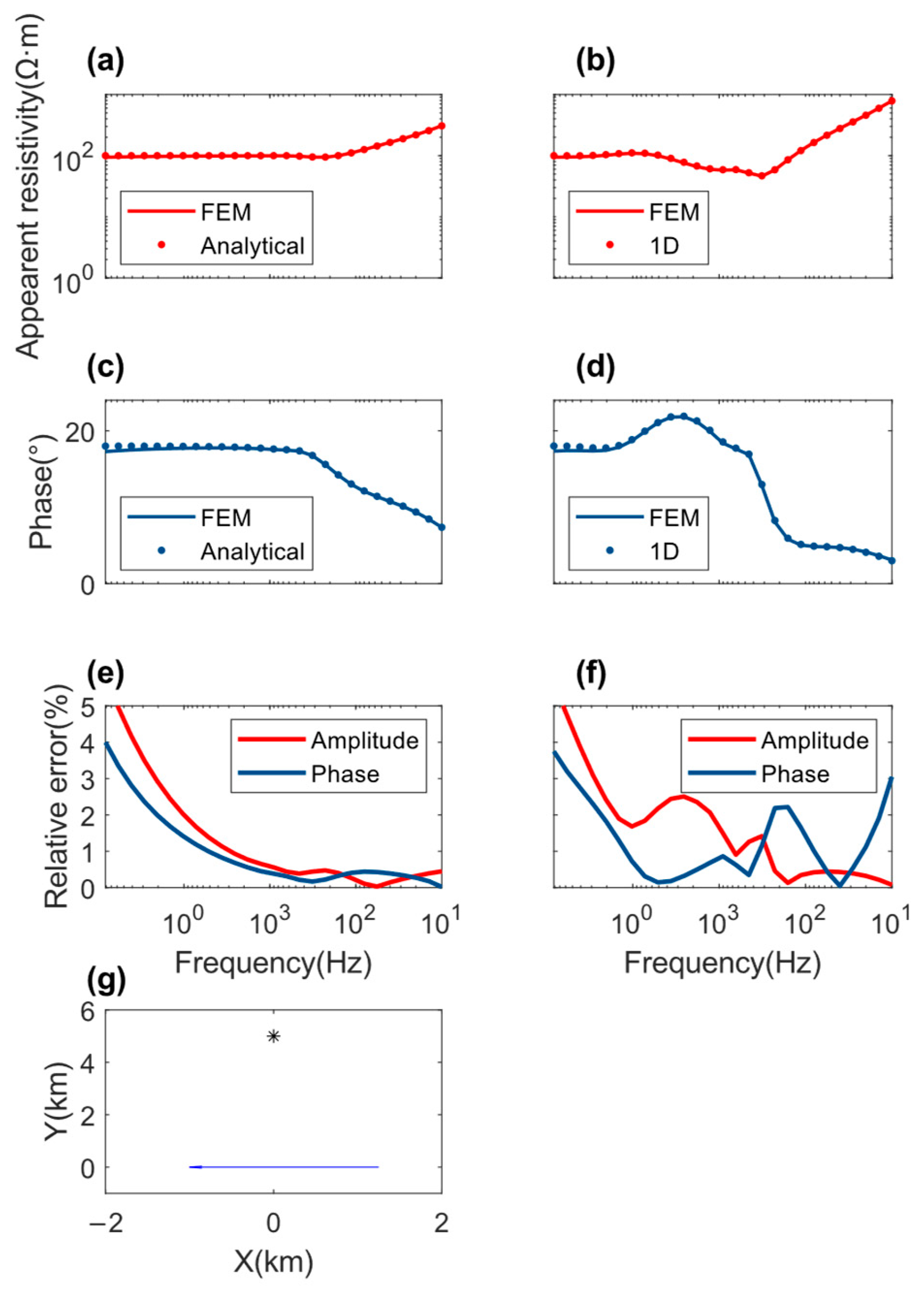
2.1. Controlled-Source Audio-Frequency Magnetotelluric (CSAMT) Forward Modeling

This section derives the CSAMT forward modeling equations from Maxwell’s equations. Our modeling approach draws inspiration from the open-source project MARE2DEM by Kerry Key [36], a robust parallelized modeling tool. For further theoretical details, see the work of Mitsuhata [37], which provides the foundational principles. The quasi-static approximation of Maxwell’s equations in the frequency domain is expressed as follows:

$$\nabla \times \mathit{E}-i\mathsf{\omega }\mathsf{\mu }\mathit{H}={\mathit{M}}^s$$

(1)

$$\nabla \times \mathit{H}-\mathsf{\sigma }\mathit{E}={\mathit{J}}^s$$

(2)

where $\mathit{E}$ and $\mathit{H}$ are the electric and magnetic fields, respectively; ${\mathit{J}}^s$ is the source current density; ${\mathit{M}}^s$ is the source magnetic moment; $\mathsf{\mu }$ is the magnetic permeability; $\mathsf{\epsilon }$ is the dielectric constant; and $\mathsf{\sigma }$ is the conductivity.

For 2.5D forward modeling, we assume that the subsurface does not vary in the $y$ direction and apply a Fourier transformation along this axis; thus, we obtain the following equation:

$$-\nabla \cdot \left(p{k}_e^{-2}\nabla {\widehat{e}}_y^s\right)-i{k}_y\nabla \cdot \left(p{k}_e^{-2}\nabla {\widehat{h}}_y^s\right)+p{\widehat{e}}_y^s={\widehat{S}}_1$$

(3)

$$-\nabla \cdot \left(q{k}_e^{-2}\nabla {\widehat{h}}_y^s\right)-i{k}_y\nabla \cdot \left(q{k}_e^{-2}\nabla {\widehat{e}}_y^s\right)+q{\widehat{h}}_y^s={\widehat{S}}_2$$

(4)

where

$$\begin{array}{l}p=\mathsf{\sigma }+i\mathsf{\epsilon }\mathsf{\omega }; q=i\mathsf{\mu }\mathsf{\omega }; k_e^2=k_y^2+pq;\\ {\widehat{S}}_1=-{ \widehat{\mathit{J}}}_{py}+i{k}_y\nabla \cdot \left(k_e^{-2}{ \widehat{\mathit{J}}}_{pt}\right)-\nabla \cdot \left(pq{k}_e^{-2}{ \widehat{\mathit{M}}}_{pt}\right)\\ {\widehat{S}}_2=-q{ \widehat{\mathit{M}}}_{py}+i{k}_y\nabla \cdot \left(q{k}_e^{-2} {\widehat{\mathit{M}}}_{pt}\right)-\nabla \cdot \left(q{k}_e^{-2}{ \widehat{\mathit{J}}}_{pt}\right)\end{array}$$

(5)

where ${\widehat{e}}_y^s$ and ${\widehat{h}}_y^s$ represent the electric field intensity and magnetic field intensity in the $y$ direction, $k_y$ is the wavenumber in the $y$ direction, $\mathsf{\omega }$ is the angular frequency, and ${\widehat{S}}_1$ and ${\widehat{S}}_2$ are the source terms. ${ \widehat{\mathit{J}}}_{pt}$ and ${ \widehat{\mathit{M}}}_{pt}$ represent the electric current density and magnetic moment vectors perpendicular to the $y$ direction, respectively. Correspondingly, ${ \widehat{\mathit{J}}}_{py}$ and ${ \widehat{\mathit{M}}}_{py}$ represent the electric current density and magnetic moment vectors parallel to the $y$ direction, respectively.

We use an unstructured adaptive triangular mesh combined with first-order shape functions to solve the finite-element problem, applying Dirichlet boundary conditions at the boundaries. Additionally, we use the Gauss–Legendre integration method to discretize the finite-length transmitter wire into multiple electric dipoles, each computing the response, which are then summed with different coefficients. As a result, $\widehat{\mathit{M}}$ can be neglected. The forward model is placed at the center of a square extension model with a side length of 60,000 m. We perform the triangular meshing using the open-source Gmsh library [38] and refine the mesh near the receiver and transmitter to improve the computational accuracy. The triangle edge lengths increase with their distance from the center, reducing the number of elements while maintaining accuracy and accelerating the computation speed.

After applying the boundary conditions, we note that the equation solutions for different wavenumbers and frequencies are independent of each other, enabling parallel computation. For single-frequency and wavenumber solutions, we use the serial version of the Math Kernel Library (MKL) Pardiso. Furthermore, in the following study, we employ parallel tempering to execute the MCMC algorithm, which is also a parallel technique. Thus, our Bayesian inversion uses double parallelism, utilizing as many cores as possible to shorten the computational time. Next, the values for other directions are calculated using ${\widehat{e}}_y^s$ and ${\widehat{h}}_y^s$, and then the results are converted from the wavenumber domain to the spatial domain using the inverse Fourier transformation. Since the finite-element method uses an unstructured mesh, the grid can closely follow the topography, and the air above the surface is assigned a resistivity of ${10}^8 \mathrm{\Omega }\cdot \mathrm{m}$.

Before using this forward modeling for inversion, we must first validate its correctness. In this study, we use Carniard resistivity as the observed target response, with the following calculation formula:

$$\begin{array}{l}{\mathsf{\rho }}_s={\displaystyle \frac{1}{\mathsf{\omega }\mathsf{\mu }}}\cdot {\displaystyle \frac{{\left|E_p\right|}^2}{{\left|H_t\right|}^2}}\\ \mathsf{\phi }={\mathsf{\phi }}_{E_p}-{\mathsf{\phi }}_{H_t}\end{array}$$

(6)

where $E_p$ represents the electric field component parallel to the direction of the transmitting electric dipole, $H_t$ represents the magnetic field component perpendicular to the transmitting electric dipole, and $\mathsf{\phi }$ is the phase angle.

Model 1 is a homogeneous half-space model, and the comparison method used is the analytical solution of the dipole integration along the wire direction. For Model 1, the transmitting wire is parallel to the $y$ direction and perpendicular to the survey line direction, with resistivity $\mathsf{\rho }=100 \mathrm{\Omega }\cdot \mathrm{m}$. The transmitter has a value of $2500 \mathrm{m}\times 1\mathrm{A}$, and is located at the center coordinate (0, 0), and the receiver is located at (0, 5000). The predicted receiver response and comparison error are shown in Figure 1a,c. We also performed a comparison between the finite-element solution and the 1D model (Model 2) numerical solution [39]. Model 2 consists of four layers with the resistivities ${\mathsf{\rho }}_1=100 \mathrm{\Omega }\cdot \mathrm{m}$, $h_1=200 \mathrm{m}$, ${\mathsf{\rho }}_2=20 \mathrm{\Omega }\cdot \mathrm{m}$, $h_2=100 \mathrm{m}$, ${\mathsf{\rho }}_3=500 \mathrm{\Omega }\cdot \mathrm{m}$, $h_3=200 \mathrm{m}$, and ${\mathsf{\rho }}_4=200 \mathrm{\Omega }\cdot \mathrm{m}$, and the transmitter and receiver settings are the same as those in Model 1. The predicted receiver response and comparison error are shown in Figure 1b,d.

As shown in Figure 1, the computational error of the finite element solution is within an acceptable range, which is sufficient to support our inversion study.

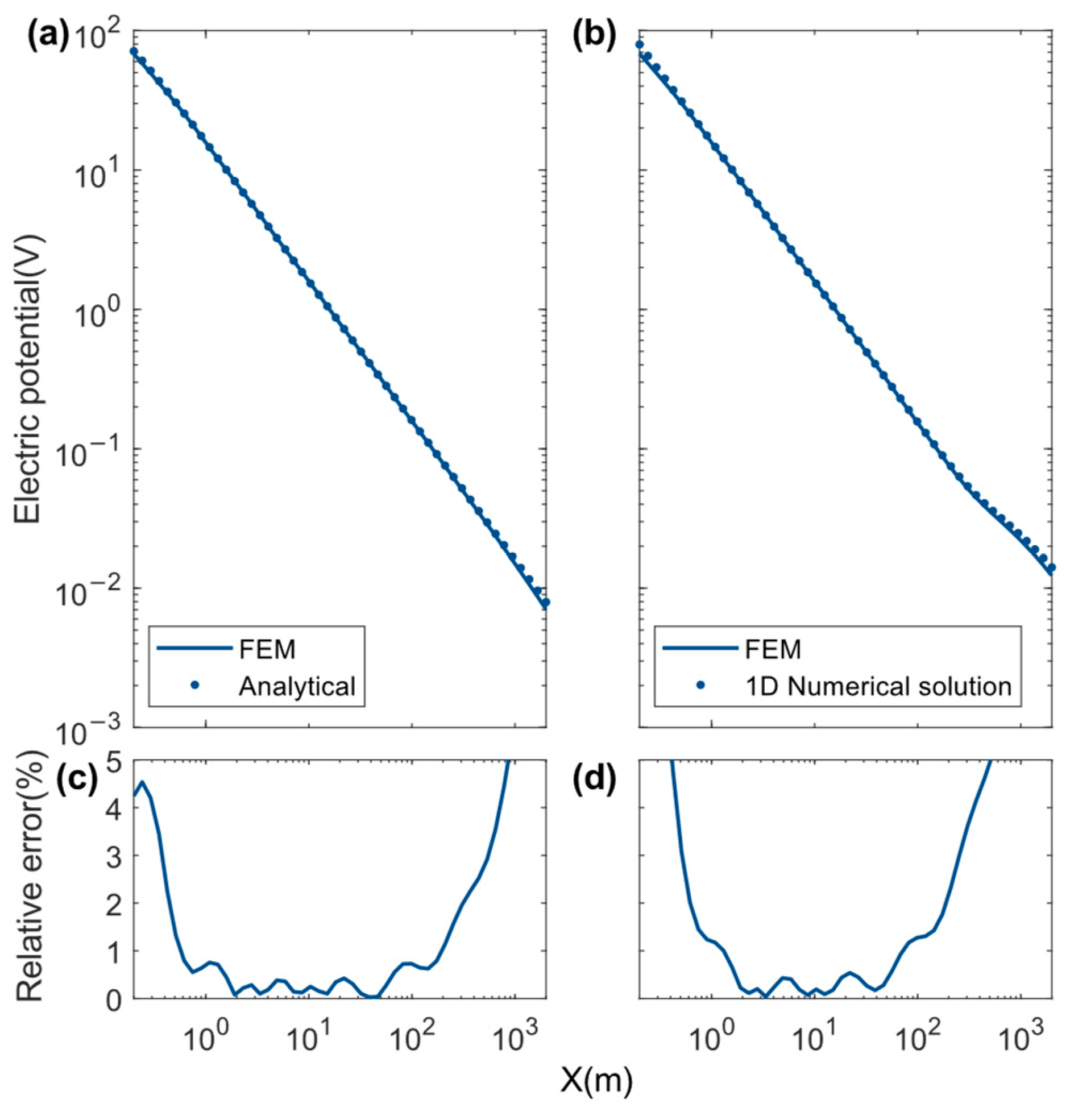
2.2. Direct Current (DC) Forward Modeling

The DC forward modeling also uses a 2.5D approach, where the boundary value problem for the steady-state current field potential is given by:

$$\begin{array}{c}\nabla \cdot (\mathsf{\sigma }\nabla u)=-2I\mathsf{\delta }(x), \in \mathrm{\Omega }\\ {\displaystyle \frac{\mathsf{\partial }\mathrm{u}}{\mathsf{\partial }n}}=0, \in {\mathsf{\Gamma }}_s\\ u={\displaystyle \frac{c}{r\prime }}, \in {\mathsf{\Gamma }}_{\infty }\end{array}$$

(7)

where $\nabla$ is the Hamiltonian operator, $\mathsf{\sigma }$ is the conductivity, $u$ is the potential, $I$ is the current, $\mathsf{\delta }(x)$ is the Dirac delta function centered at $x$, ${\mathsf{\Gamma }}_s$ represents the surface boundary, ${\mathsf{\Gamma }}_s$ represents the boundary at infinity, $r\prime$ is the distance from the source to the boundary, $\mathrm{\Omega }$ is the model area, and $c$ is the potential value at the point power source.

For the 2D resistivity problem, a Fourier transformation is applied along the $y$ direction using Equation (7), transforming the 3D boundary value problem into a 2D boundary value problem in the wavenumber domain.

$$\begin{array}{c}\nabla \cdot (\mathsf{\sigma }\nabla u)-k_y^2\mathsf{\sigma }u=-I\mathsf{\delta }(x), \in \mathrm{\Omega }\\ {\displaystyle \frac{\mathsf{\partial }\mathrm{u}}{\mathsf{\partial }n}}=0, \in {\mathsf{\Gamma }}_s\\ {\displaystyle \frac{\mathsf{\partial }\mathrm{u}}{\mathsf{\partial }n}}+k_y{\displaystyle \frac{K_1\left(k_{y}r\right)}{K_0\left(k_{y}r\right)}}\cos \left(r,n\right)u=0, \in {\mathsf{\Gamma }}_{\infty }\end{array}$$

(8)

where $k_y$ represents the wavenumber in the $y$-direction, which is completely consistent with that in Equations (3)–(5), $K_0$ is the modified Bessel function of the second kind of order zero, and $K_1$ is the modified Bessel function of the second kind of order one. Nine specific wavenumbers are selected for forward modeling, and the potential signal is restored from the wavenumber domain to the spatial domain using weighted summation integration.

Dirichlet boundary conditions are applied, assuming the potential is zero at the boundary. An unstructured triangular finite-element mesh method is also employed. Following the work of Xu et al. [40], an optimized discretization method is used, with the wavenumbers $k_y$ = [0.000167741, 0.000891545, 0.00319213, 0.0113809, 0.0422622, 0.162549, 0.645985, 2.65801, 11.3951] being selected, with the corresponding coefficients g = [0.000257473, 0.000760986, 0.0025502, 0.00935952, 0.0357988, 0.141072, 0.574423, 2.42421, 10.8104]. After calculating the results for each wavenumber, they are weighted and summed to obtain the point-source result for the 2D model. The forward model is set up similarly to the CSAMT method, being positioned at the center of a square extension model with a side length of 60,000 m. The air above the ground is assigned a resistivity of ${10}^8 \mathrm{\Omega }\cdot \mathrm{m}$, and mesh refinement is applied at electrode locations to improve the accuracy of the solution. Given the independence of the equations for different wavenumbers, a parallel solution algorithm is developed, similar to the approach used for CSAMT.

Figure 2 compares the DC forward modeling program used in this study with the analytical solution [41] and the 1D numerical solution [42]. The model resistivity settings are the same as in Figure 1, with a single-point transmitter located at (0, 0).

As shown in Figure 2, the computational error of the finite element solution is within an acceptable range. For the finite element method, near the transmitter, the error increases due to the presence of singularities at the source location [43]. Upon verification, the finite element solution used in this study, using the aforementioned nine wavenumbers, has an error of less than 6% within a distance range of 0.4–2000 m from the source, which is sufficient to support the subsequent inversion work.

2.3. Bayesian Inversion

Here, our Bayesian inversion uses MCMC sampling to estimate the posterior probability distribution. The Bayesian theorem, incorporating prior knowledge, can be expressed as [44]:

$$P\left(\mathit{m} | \mathit{d}\right)={\displaystyle \frac{P\left(\mathit{m}\right)P\left(\mathit{d} | \mathit{m}\right)}{P(\mathit{d})}}$$

(9)

where $P\left(\mathit{m}\right)$ is the probability density function of the model parameters, $P\left(\mathit{d} | \mathit{m}\right)$ is the likelihood of the model given the observed data, and $P\left(\mathit{m} | \mathit{d}\right)$ is the posterior probability density function (pdf), which is the inversion result we seek. From this, the expectation and uncertainty of the inversion model can be derived. $P(\mathit{d})$ is the Bayesian evidence, a constant that normalizes the posterior probability.

In this study, we use available rock resistivity data to constrain the prior probability distribution of the resistivity model. Based on this, we apply a geostatistical random modeling approach [25] to construct a 2D subsurface resistivity model. We selected a Gaussian-type variogram as the prior method for random geological modeling and the fast Fourier transform moving average (FFTMA) algorithm as the prior modeling method. The Gaussian-type variogram generates smoother prior models, which are well-suited for electromagnetic inversion, while the FFTMA algorithm is more efficient than other methods [27]. Additionally, the model parameters are defined by the actual measured rock resistivity probability distribution, and distribution mapping techniques are used to ensure that the prior model probabilistically reflects the likelihood of actual resistivity values [27].

For the likelihood, we assume that the data errors have a mean of zero and follow a Gaussian distribution.

$$P\left(\mathit{d} | \mathit{m}\right)={\displaystyle \frac{1}{\sqrt{{\left(2\pi \right)}^N\left|C_d\right|}}}\exp \left\{-{\displaystyle \frac{\Delta {\mathit{d}}^T{C}_d^{-1}\Delta \mathit{d}}{2}}\right\}$$

(10)

where $\mathit{d}$ represents the observed data, with $\Delta {\mathit{d}}^T$ denoting the transpose of the ${\mathit{d}}^T$ vector, $N$ is the total number of observed data, and $C_d$ is the covariance matrix of the noise in the observed data. Following the work of Long Zhidan et al. [45], we define the relative error $\Delta \mathit{d}$ as:

$$\Delta \mathit{d}=\left(\begin{array}{c}{\displaystyle \frac{{\mathit{d}}_{\mathrm{Carnia}}\left(\mathit{m}\right)-{\mathit{d}}_{\mathrm{Carnia}}}{{\mathit{d}}_{\mathrm{Carnia}}}}\\ {\displaystyle \frac{{\mathit{d}}_{\mathrm{phase}}\left(\mathit{m}\right)-{\mathit{d}}_{\mathrm{phase}}}{{\mathit{d}}_{\mathrm{phase}}}}\end{array}\right)$$

(11)

Equation (11) is composed of the relative errors in both the amplitude and phase of the Carniard resistivity, where $\mathit{d}\left(\mathit{m}\right)$ represents the data obtained from forward modeling.

We use the Metropolis–Hastings (M–H) algorithm, combined with parallel tempering [46,47], to effectively sample the model parameter space. This algorithm allows multiple chains with different temperatures to run simultaneously, enabling information exchange between the chains. Low-temperature chains perform more refined sampling, while high-temperature chains conduct broader searches. This approach helps to effectively reduce the burn-in iteration count. However, the computational cost of this algorithm is significant, typically requiring over 10⁶ forward simulations, which is impractical for conventional serial computation. Fortunately, in each iteration of parallel tempering, the model walk, forward computation, and within-chain state transitions for each temperature chain are independent, with inter-chain communication occurring only during temperature exchanges. This allows the temperature chains to advance in parallel within a single iteration. By further integrating this approach with parallelized forward modeling, dual-level parallel computing can be implemented on a cluster, significantly reducing the computation time. We ran all the computational cases presented in this study on a cluster with three nodes. Each node includes two Intel Xeon Gold 6248R 3.0 GHz processors, each with 24 physical cores. Compared to serial computation, the use of 144 cores resulted in a 73.74-fold speedup.

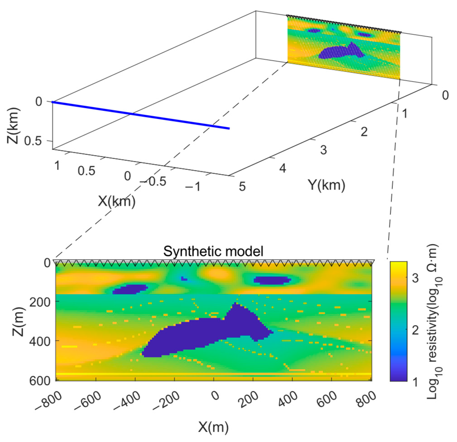
3. Synthetic Results

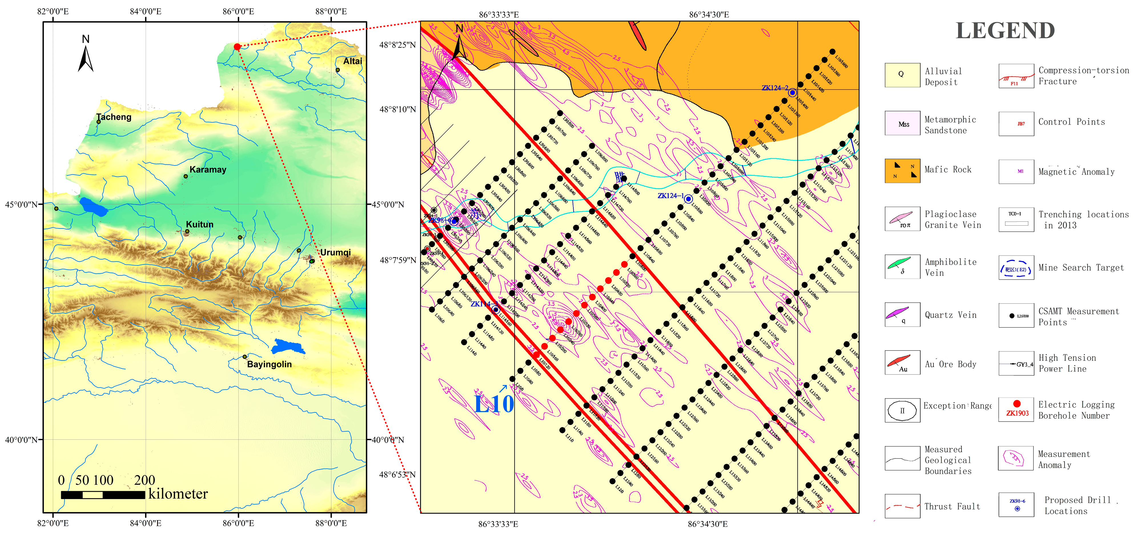
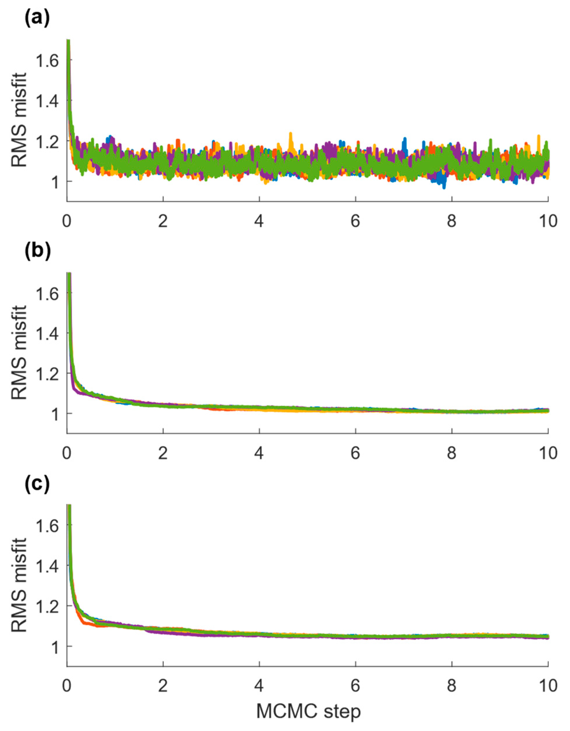
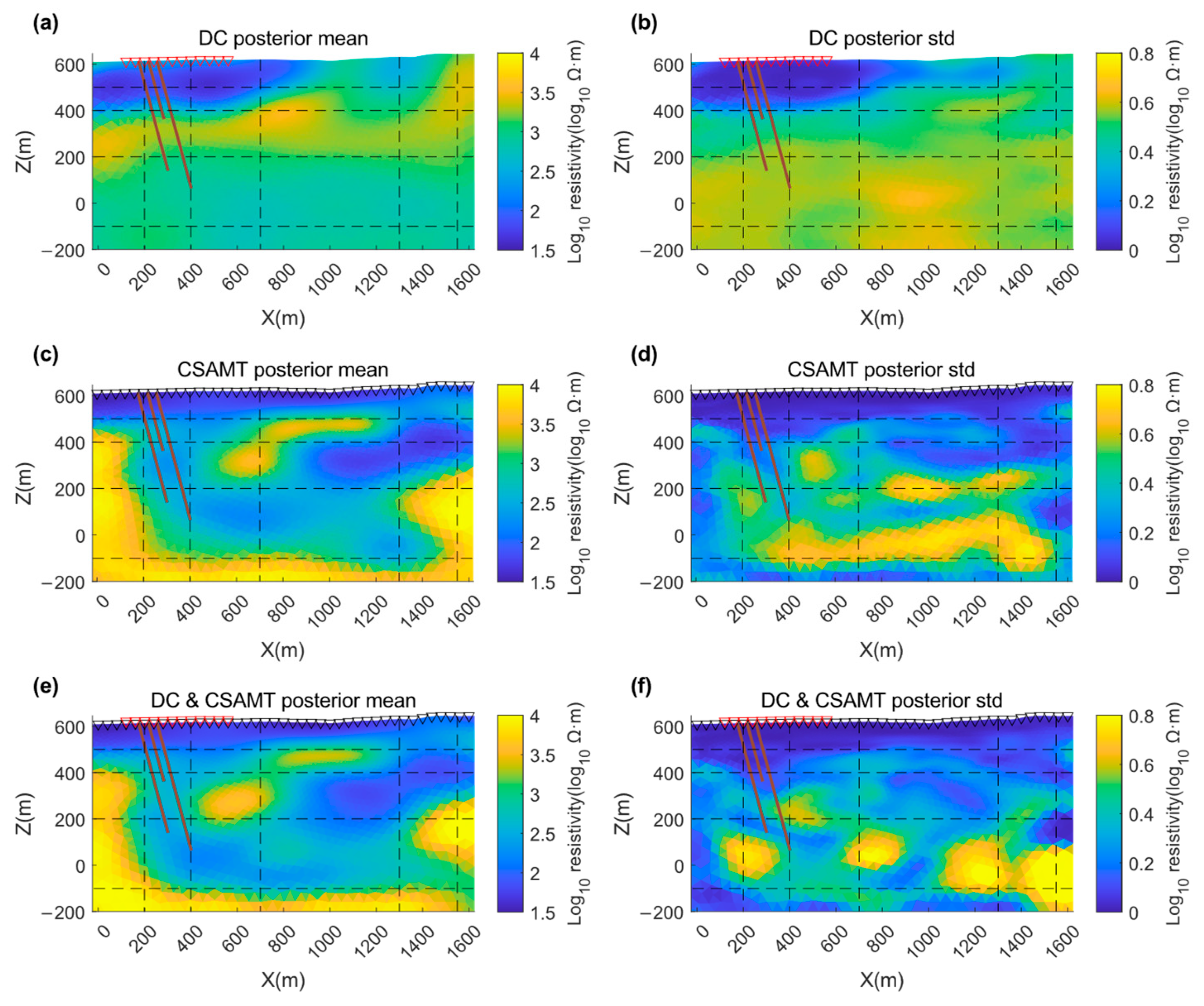
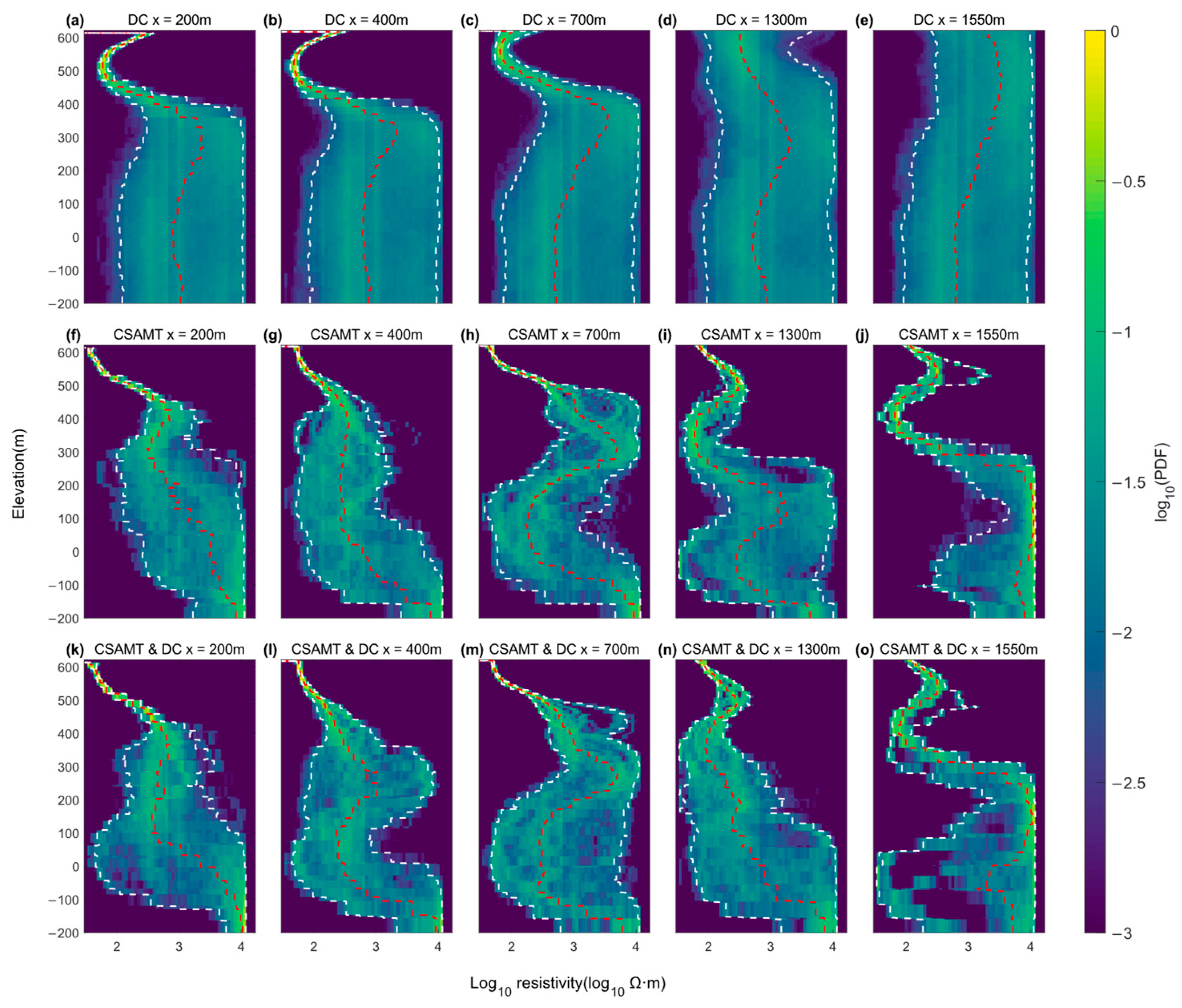
Synthetic data experiments were conducted using CSEM and DC data which were forward-modeled based on a 2D resistivity model (from MARE2DEM). The selected model is shown in Figure 3, and it is derived from the open-source salt dome model of SEG/EAGE [48,49], with some modifications. We scaled down the model and added a randomly generated geological layer at the surface, which contains two smaller salt bodies. The resistivity of three of the observed larger salt bodies is defined as 10 $\mathrm{\Omega }\cdot \mathrm{m}$, while the resistivity of the basement is heterogeneous, with a mean value of approximately 525 $\mathrm{\Omega }\cdot \mathrm{m}$. We selected a slice from the 3D model at y = −557.5 m as the subsurface model for this study.

A 2.5 km-long grounded wire is used as the transmitter, and its direction of emission is parallel to the x-axis. The distance between the transmitter and the survey line is 5 km. The locations of the observation stations are marked by $\nabla$, with a total of 41 measurement points spaced 40 m apart. The measurement frequencies range from 1 Hz to 8192 Hz in a geometric progression, covering 27 frequencies. Combined with Carniard resistivity and phase measurements, this results in a total of 2214 observed data points. For the DC observations, 11 electrode spacings are used, specifically AB/2 = [50, 100, 150, 200, 250, 350, 500, 750, 850, 950, 1000] m, leading to a total of 451 observed data points. All simulated observation data were contaminated with 3% Gaussian white noise.

For the prior resistivity information of the region, we assume that detailed and comprehensive rock resistivity data have been collected using logarithmic resistivity (base 10) as the model parameter. The regional resistivity distribution $10\%N(1,{0.05}^2)+90\%N(2.6,{0.18}^2)$ is defined as a prior distribution, which is a combination of two Gaussian distributions: 10% of the data has a mean of 1 and a standard deviation of 0.05, and 90% of the data has a mean of 2.6 and a standard deviation of 0.18. All values are expressed as logarithmic resistivity. The comparison between the actual logarithmic resistivity probability distribution and the prior setting is shown in Figure 4. As can be seen, there is still a significant difference between the two, particularly in the low-resistivity portion. The inversion uses a Gaussian-type variogram as the prior model, with an autocorrelation radius of 200 m in the vertical direction and a horizontal autocorrelation radius that is 2.2 times that of the vertical direction. The comparison between the prior variogram and the actual data is shown in Figure 5. It should be noted that the DC-only inversion, CSAMT-only inversion, and DC and CSAMT joint inversion all use the same prior setup to eliminate the influence of different priors on the posterior results, making it easier to explore the differences caused solely by the choice of detection method. The inversion grid setup is different from the forward modeling setup, and we have also added 1% uncorrelated model error noise to the inversion’s noise model [50] to prevent overfitting of the model.

The Bayesian inversion uses 16 Markov chains, with 5 chains at temperature T = 1. Each chain is allocated nine cores. A total of 100,000 iterations were performed, with the first 50,000 iterations discarded as burn-in. For explanations on temperature and burn-in, please refer to the studies of Sambridge and Malcolm [46] and Hansen et al. [47,51]. The changes in the RMS misfit are shown in Figure 6. In the end, 83,333 posterior sample models were collected. The data mismatch for all models in the posterior set follows a distribution of ${\mathsf{\chi }}^2$, with average RMS mismatches of 1.133 (DC), 0.9864 (CSAMT), and 1.243 (DC and CSAMT). The posterior statistical results are shown in Figure 7. The locations of the salt bodies are marked with a red solid line, and the area marked by white dashed lines indicates areas where at least 50% of the samples have resistivity values lower than 20 $\mathsf{\Omega }\cdot \mathrm{m}$. To further explore the differences between the joint inversion and single geophysical field inversion in terms of their posterior results, Figure 8 shows the marginal posterior densities along a depth profile for the points of interest, and Figure 9 displays the marginal posterior densities along a lateral profile at specific depths. The locations of these profiles are marked by black dashed lines in Figure 6. In these figures, the shaded area represents the relative likelihood of the logarithmic resistivity shown at each depth. The median is represented by a red dashed line, and the minimum and maximum values of the 95% highest posterior density (HPD) are indicated by green dashed lines.

Comparing the posterior mean with the simulated model, both the single-method and joint inversions successfully captured the three large salt bodies. However, the single DC inversion provided inaccurate predictions for the salt bodies, exhibiting vertical stretching in the results. We hypothesize that this distortion arises from a mismatch between the prior and the actual model structure. The model consists of two submodels with different correlation lengths, whereas the inversion assumes a uniform prior correlation length that is larger than the actual correlation length in the shallow region. Additionally, the DC dataset is relatively small, comprising only 451 observations, which is far fewer than the number of model parameters. As a result, the influence of the prior model on the inversion results is amplified. The actual autocorrelation length in the shallow region is 80 × 240, which is smaller than the prior assumption of 200 × 440. While Bayesian inference can refine the prior model to better align with the posterior model, it cannot fully correct this bias.

The CSAMT dataset is approximately five times larger than the DC dataset, enabling a more significant correction of the prior. Consequently, the single CSAMT inversion provides more accurate localization of the three salt bodies. Figure 8 and Figure 9 illustrate that, in the shallow region (within 200 m depth), the posterior shape in the single CSAMT inversion deviates more from the true model than that in the single DC inversion. Additionally, the confidence interval is broader in this depth range. However, as the depth increases, the imaging capability of the CSAMT method gradually surpasses that of the DC resistivity method.

A direct comparison of Figure 7c,e indicates that the improvements in the joint inversion over the single CSAMT inversion are relatively limited. However, Figure 7d,f demonstrate that the primary advantage of joint inversion lies in the reduction in uncertainty. The joint inversion exhibits narrower high-posterior standard deviation (posterior std) regions along the salt body edges, and the HPD interval width is slightly smaller than that of either single-method inversion. The incorporation of additional data allows the likelihood function to refine the prior more effectively.

The contribution of different datasets to the inversion model is not uniform. Figure 8 and Figure 9 show that, in shallow depths (<100 m), the joint inversion results more closely resemble those of the DC inversion than the CSAMT inversion, whereas the overall model is more aligned with the CSAMT results. This suggests that CSAMT plays a dominant role in the joint inversion, influencing the entire model, whereas the DC data primarily enhance the shallow imaging. The joint inversion increases the data volume by approximately 20% compared to the single CSAMT inversion. However, this increase does not result in a significant improvement in the inversion results. Instead, its primary effect is that the DC data assist the CSAMT method in eliminating certain incorrect shallow models, thereby indirectly helping to reduce uncertainty in the deeper regions of the CSAMT inversion.

4. Field Results

In this study, we apply the developed methods and algorithms to address a practical gold vein exploration problem. The study area is a gold mine located in Xinjiang, China. Figure 10 shows the location of the survey area and part of the survey design.

We selected one survey line, L10, which crosses two suspected mineral veins on the map. The specific exploration setup is shown in Figure 11, where the L10 survey line is marked at y = 0 on the map. Black dots represent the CSAMT measurement points, and red dots represent the DC depth measurement points. For display purposes, the black and red dots are slightly offset in the vertical direction, but in the actual measurements, they coincide. The remaining unused survey lines are marked with solid black lines. The CSAMT transmitter is located approximately 12 km northwest of the survey line and is marked with a blue solid line. It is a 2.5 km-long grounded wire, placed parallel to the survey line direction. The CSAMT data were collected using the Phoenix V8 system (Phoenix Geophysics Limited, Toronto, ON, Canada), with 43 frequencies selected logarithmically from 1 Hz to 7680 Hz. The survey line is 1600 m long, with 40 m spacing between measurement points and a total of 41 receivers. The inversion data each include the Carniard resistivity and the corresponding phase, totaling 3526 data points. The DC data were collected using the ZONGE GDP32 system (Zonge International, Inc., Tucson, AZ, USA). Due to practical limitations, the DC survey line is 440 m long and overlaps with the CSAMT survey line from 120 m to 560 m. A symmetric dipole array was used, with 11 electrode spacing sequences for AB/2 at distances of 50, 100, 150, 200, 250, 350, 500, 750, 850, 950, and 1000 m. The MN/2 length is one-fifth of AB/2. The measurement points are spaced 40 m apart, with 12 observation points, resulting in a total of 132 DC data points. For survey lines of the same length, the DC data represent only 13% of the CSAMT data. Considering the 3D effects and other factors in data inversion, the noise level for both the DC and CSAMT data was set to 10%.

Before proceeding with the inversion, we collected 216 rock samples from the survey area and measured their resistivities. These samples were obtained from borehole cores and surface collections. Using these in conjunction with other rock resistivity data previously collected by other teams in the survey area, we compiled the statistical data shown in

Table 1. Rock resistivity statistics.

Serial Number	Rock Name	Measurement Location	Number of Measurements	Resistivity (log10 Ω·m)
				Mean Value	Standard Deviation	Minimum Value	Maximum Value	Measurement Time
1	Altered Sandstone	Tunnel Wall	15	2.8048		2.4183	3.4064	2020
2	Pyrite-Quartz Vein	Tunnel Wall	23	3.9729		2.9996	4.5013
3	Altered Sandstone	Pit Wall	5	1.3617		1.2788	1.4314
4	Diorite	Surface Exposure	5	2.1614		2.0792	2.2355
5	Granite	Surface Exposure	6	3.1326		2.2068	3.6479
6	Phyllite	Surface Exposure	5	1.5563		1.1461	1.8633
7	Ore-bearing Diorite	Pit Wall	5	2.4346		2.3222	2.5490
8	Altered Sandstone	Tunnel Wall and Borehole	6	4.1105		2.8609	4.4044	2021
9	Granite	Tunnel Wall and Borehole	5	4.2560		3.4982	4.6711
10	Pyritized Altered Sandstone	Tunnel Wall	5	3.6950		3.2068	4.1164
11	Pyritized Granite	Tunnel Wall	5	4.1525		3.8223	4.4017
12	Pyritized Phyllite	Tunnel Wall	5	3.9982		2.6884	4.3557
13	Pyritized Diorite	Tunnel Wall	5	3.5344		1.6990	3.7301
14	Pyritized Quartz Vein	Tunnel Wall	5	3.4089		2.8531	3.8182
15	Amphibolite	Borehole	4	3.2310		3.0849	3.4173
16	Phyllite	Tunnel Wall	5	4.2262		3.3955	4.5936
17	Diorite	Tunnel Wall	5	3.5359		2.7752	3.7877
18	Quartz Vein	Tunnel Wall	6	3.5660		3.0924	3.9687
19	Monzonite	Borehole	8	4.0683		3.5532	4.4537
20	Altered Sandstone		28	3.0911		2.0043	3.9283	2021
21	Biotite Quartz Schist		83	3.2020		2.1553	3.9258
22	Ore-bearing Diorite	Ore	33	3.4261		2.7364	4.7516
23	Diorite	Borehole	15	3.0479		1.6628	4.3136
24	Granite		86	3.5928		2.1004	5.0541
25	Monzonite		23	3.7907		3.3066	4.2302
26	Quartz Vein-bearing Altered Sandstone	Surface Exposure	7	3.8736		2.5211	5.0086
27	Pyrite-Quartz Vein		5	3.9729		2.9996	4.5013
28	Metamorphic Sandstone	Surface Exposure and Borehole	21	2.9600		1.9494	3.3300	2022
29	Biotite Schist	Surface Exposure and Borehole	4	2.9832		2.6590	3.2230
30	Pyritized Diorite	Surface Exposure and Borehole	6	2.7340		2.4983	3.0004
31	Sericite Green Clay Phyllite	Surface Exposure and Borehole	6	2.7275		2.2672	2.9513
32	Phyllite	Surface Exposure and Borehole	26	2.8241		2.1959	3.1998
33	Diorite	Surface Exposure and Borehole	17	2.6928		1.9956	3.1096
34	Altered Diorite	Surface Exposure and Borehole	14	2.7910		2.2989	3.1735
35	Carbonatized Metamorphic Rock	Surface Exposure and Borehole	3	2.9154		2.2175	3.1316
36	Granite	Surface Exposure and Borehole	16	3.1556	0.2295	2.8831	3.7067	2024
37	Coarse-grained Granite	Surface Exposure and Borehole	22	3.1308	0.2464	2.6812	3.5562
38	Phyllite	Surface Exposure and Borehole	17	3.3762	0.2962	2.7419	3.9645
39	Silicified Phyllite	Surface Exposure and Borehole	7	3.4736	0.4196	3.0945	4.1859
40	Diorite	Surface Exposure and Borehole	31	3.1261	0.2931	2.6395	3.8289
41	Pyrite-bearing Diorite A	Surface Exposure and Borehole	21	2.5146	0.1673	2.1820	2.8301
42	Pyrite-bearing Diorite B	Surface Exposure and Borehole	11	3.1886	0.1885	3.0001	3.4656
43	Quartzite	Surface Exposure and Borehole	22	3.0927	0.4125	2.4518	3.8254
44	Pyrite-bearing Quartzite	Surface Exposure and Borehole	5	2.6091	0.2806	2.1128	2.9737

, which only presents the statistics for the main types of rock in the region and excludes data for minor rock types.

The statistical results show that the logarithmic resistivity of the rocks in the survey area follows a distinct Gaussian distribution, with the resistivity values mainly being concentrated in the range of [100, 8000] $\mathsf{\Omega }\cdot \mathrm{m}$ and having a mean value of approximately 3000 $\mathsf{\Omega }\cdot \mathrm{m}$. Based on the geological data of the survey area, over 70% of the region consists of schist, with mineralized target rocks that are primarily composed of metamorphic diorite and metamorphic quartz sandstone accounting for about 20%, while other rock types make up less than 10%. Based on the study by Blatter et al. [52], there is a strong correlation between the resistivity of a rock and its water content. Fortunately, deep-seated diorite, granite, and quartzite are typically dense with very low porosity, meaning their resistivity is unlikely to undergo significant variations due to water saturation. In contrast, schist, due to its layered structure and relatively higher porosity, exhibits greater sensitivity to water content variations. This is also reflected in Table 1, where the logarithmic resistivity standard deviation for schist is the largest, exceeding that of the other rock types. Although no surface water flow is observed in the study area, the possibility of water-bearing fractured zones or weathered layers in the shallow subsurface cannot be ruled out. As a result, unexpected shallow low-resistivity anomalies may still appear. Considering these factors, we define the logarithmic resistivity as the inversion target and set the prior distribution as $10\%N(2.7,{0.32}^2)+20\%N(3,{0.38}^2)+70\%N(3.36,{0.45}^2)$, covering the [100, 20,000] $\mathsf{\Omega }\cdot \mathrm{m}$ resistivity range. This ensures that the prior model is sufficiently broad while avoiding significant bias in the inversion process.

We performed three inversions using the collected data: single DC inversion, single CSAMT inversion, and joint DC and CSAMT inversion. Figure 12 illustrates the RMS misfit variation trends for the three inversions. Figure 13 presents the logarithmic resistivity probability distribution of the posterior sample sets from each inversion, comparing them to their prior logarithmic resistivity distributions. Figure 14 displays the inversion results for all three cases. Compared to the prior distribution, the different inversions modify the resistivity distribution in distinct ways, with consistent trends, and show varying degrees of concentration at the locations ${10}^{1.8}\mathsf{\Omega }\cdot \mathrm{m}$, ${10}^{2.5}\mathsf{\Omega }\cdot \mathrm{m}$, and ${10}^4\mathsf{\Omega }\cdot \mathrm{m}$. Based on the data in Table 1, we infer that the peak at ${10}^{2.5}\mathsf{\Omega }\cdot \mathrm{m}$ corresponds to pyrite-rich diorite A or pyrite-rich quartzite, that the peak at ${10}^4\mathsf{\Omega }\cdot \mathrm{m}$ corresponds to schist or silicified schist, and that the peak at ${10}^{1.8}\mathsf{\Omega }\cdot \mathrm{m}$ is unexplained by any rock due to having such a low resistivity, suggesting it may be due to a fractured zone filled with water.

Near the survey line, we identified three boreholes, named K1–K3 from left to right, which are laterally offset by less than 10 m from the survey line and extend downward at an angle of 75°. These boreholes are located within the overlapping measurement area of the DC and CSAMT data, providing strong validation for the borehole data’s validity and accuracy. According to the borehole reports, the core consistency across all three boreholes is very high. The overlying quaternary cover, less than 20 m thick, quickly transitions to gravel and fractured zones which are highly heterogeneous and composed of quartzite, granite, diorite, schist, chlorite, biotite, and other minerals. As the depth increases, the layers stabilize beyond 80 m, alternating between pyrite-rich quartzite and diorite, with some biotite present. This is consistent with the results that can be inferred from Figure 14, further supporting the high reliability of our inversion work.

The single DC inversion in Figure 14 suggests that the depth of the low-resistivity surface may reach 200 m, but in reality it is around 80 m. A possible reason for the overestimated thickness of the upper layer in this location may be an influence of anisotropy on the DC method data. Accounting for the influence of anisotropy on the inversion results is the subject of further research. The single CSAMT inversion results maintain high credibility down to 400 m depth, revealing three distinct regions: a pyrite-rich area on the left, a high-resistivity body in the center, and a low-resistivity body on the right. In the field data inversion, the overall data error was set to 10%, compared to 4% in the theoretical model. As a result, the inversion exhibits reduced accuracy in deep resistivity estimation. Nevertheless, it is still possible to estimate a clear boundary where the resistivity changes from low to high at a certain depth. The joint inversion results are similar to the single CSAMT inversion but differ in that the joint inversion suggests that the high-resistivity anomaly in the center may be composed of two blocks rather than one, and that the uncertainty in the deep region is somewhat reduced. Figure 15 and Figure 16 both show that the advantage of joint inversion lies in the concentration of the posterior distribution, indicating reduced uncertainty. Although the DC method struggles to provide effective detection at depth, its high certainty in shallow resistivity measurements helps eliminate many incorrect solutions in the CSAMT results, indirectly improving CSAMT’s ability to detect deep features.

5. Conclusions

In this study, we successfully demonstrated the joint Bayesian inversion of DC and CSAMT data. We applied a geostatistical-based Bayesian inversion method to invert both synthetic and field data, resulting in a 2D subsurface resistivity model. By analyzing the posterior mean, standard deviation (std), and highest posterior density (HPD) of the inversion results, we examined the improvements in accuracy and uncertainty provided by joint inversion compared to single exploration methods. The results show that the joint inversion of DC and CSAMT data effectively improves the accuracy of the inversion and reduces the uncertainty of the results, combining the strengths of both methods while mitigating their weaknesses. Even under high-noise conditions, the joint inversion still significantly enhances deep imaging capabilities. In future exploration efforts, joint inversion may be used to improve our capability of detecting specific targets, especially when interference cannot be reduced.

The joint inversion of DC and CSAMT does indeed improve the imaging resolution, primarily by refining the contours of the target body. However, at present, this enhancement does not yield significant benefits for gold exploration, which may be due to the limitations of the employed geophysical methods. Utilizing techniques with larger data volumes, such as magnetotelluric (MT) or time-domain electromagnetic (TEM) methods, may potentially lead to greater improvements in imaging accuracy. We hope that future studies will further validate this hypothesis.

References

1. Løseth, L.O.; Pedersen, H.M.; Ursin, B.; Amundsen, L.; Ellingsrud, S. Low-frequency electromagnetic fields in applied geophysics: Waves or diffusion? Geophysics 2006, 71, W29–W40. [Google Scholar] [CrossRef]
2. An, Z.; Di, Q. Application of the CSAMT method for exploring deep coal mines in Fujian Province, Southeastern China. J. Environ. Eng. Geophys. 2010, 15, 243–249. [Google Scholar] [CrossRef]
3. Yang, D.; Oldenburg, D.W. Survey decomposition: A scalable framework for 3D controlled-source electromagnetic inversion. Geophysics 2016, 81, E69–E87. [Google Scholar] [CrossRef]
4. Dai, Q.-w.; Dan, D.; Biao, L.; Wu, Q.-H.; Yan, J.-B.; Hua, K.; Chen, S.-F.; Qi, Z.; Tang, Y.-Y. Deep exploration of W-Sn and Cu polymetallic deposits in middle Qin-Hang metallogenic belt, South China. Trans. Nonferrous Met. Soc. China 2023, 33, 231–253. [Google Scholar] [CrossRef]
5. Thorkildsen, V.S.; Gelius, L.-J. Electromagnetic resolution—A CSEM study based on the Wisting oil field. Geophys. J. Int. 2023, 233, 2124–2141. [Google Scholar] [CrossRef]
6. Ray, A.; Key, K.; Bodin, T.; Myer, D.; Constable, S. Bayesian inversion of marine CSEM data from the Scarborough gas field using a transdimensional 2-D parametrization. Geophys. J. Int. 2014, 199, 1847–1860. [Google Scholar] [CrossRef]
7. Wang, K.; Queralt, P.; Ledo, J.; Meqbel, N. CSEM and MT Inversion at the Hontomín CO2 Storage Site in Burgos, Spain. IEEE Trans. Geosci. Remote Sens. 2024, 62, 5922316. [Google Scholar] [CrossRef]
8. Escalas, M.; Queralt, P.; Ledo, J.; Marcuello, A. Polarisation analysis of magnetotelluric time series using a wavelet-based scheme: A method for detection and characterisation of cultural noise sources. Phys. Earth Planet. Inter. 2013, 218, 31–50. [Google Scholar] [CrossRef]
9. Yang, H.; Li, T.; Zhang, R.; Dong, X.; Zhuang, Y. 3D joint inversion of DC resistivity and time domain induced polarization with structural constraints in undulating topography. IEEE Trans. Geosci. Remote Sens. 2023, 61, 5920412. [Google Scholar] [CrossRef]
10. Bouchedda, A.; Bernard, G.; Gloaguen, E. Constrained electrical resistivity tomography Bayesian inversion using inverse Matérn covariance matrix. Geophysics 2017, 82, E129–E141. [Google Scholar] [CrossRef]
11. Loke, M.; Chambers, J.; Rucker, D.; Kuras, O.; Wilkinson, P. Recent developments in the direct-current geoelectrical imaging method. J. Appl. Geophys. 2013, 95, 135–156. [Google Scholar] [CrossRef]
12. Bortolozo, C.A.; Campaña, J.D.R.; Santos, F.A.M.D.; De Oliveira, G.S.; Porsani, J.L.; Pryer, T.; Sialounas, G. Joint Inversion of DC and TEM Methods for Geological Imaging. Pure Appl. Geophys. 2024, 181, 2541–2560. [Google Scholar] [CrossRef]
13. Sharma, R.; Vashisth, D.; Sarkar, K.; Singh, U.K. Joint Inversion of DC Resistivity and MT Data using Multi-Objective Grey Wolf Optimization. In Proceedings of the NSG 2024 30th European Meeting of Environmental and Engineering Geophysics, Helsinki, Finland, 8–12 September 2024; European Association of Geoscientists & Engineers: Utrecht, The Netherlands, 2024; pp. 1–5. [Google Scholar]
14. Liu, M.; Vashisth, D.; Grana, D.; Mukerji, T. Joint inversion of geophysical data for geologic carbon sequestration monitoring: A differentiable physics-informed neural network model. J. Geophys. Res. Solid Earth 2023, 128, e2022JB025372. [Google Scholar] [CrossRef]
15. Cheng, J.; Li, F.; Peng, S.; Sun, X.; Zheng, J.; Jia, J. Joint inversion of TEM and DC in roadway advanced detection based on particle swarm optimization. J. Appl. Geophys. 2015, 123, 30–35. [Google Scholar] [CrossRef]
16. Massoud, U.; Kenawy, A.A.; Ragab, E.-S.A.; Abbas, A.M.; El-Kosery, H.M. Characterization of the groundwater aquifers at El Sadat City by joint inversion of VES and TEM data. NRIAG J. Astron. Geophys. 2014, 3, 137–149. [Google Scholar] [CrossRef]
17. Bortolozo, C.A.; Couto, M.A., Jr.; Porsani, J.L.; Almeida, E.R.; dos Santos, F.A.M. Geoelectrical characterization using joint inversion of VES/TEM data: A case study in Paraná Sedimentary Basin, São Paulo State, Brazil. J. Appl. Geophys. 2014, 111, 33–46. [Google Scholar] [CrossRef]
18. Meqbel, N.; Ritter, O. New Advances for a joint 3D inversion of multiple EM methods. In Proceedings of the 76th EAGE Conference and Exhibition-Workshops, Amsterdam, The Netherlands, 16–19 June 2014; European Association of Geoscientists & Engineers: Utrecht, The Netherlands, 2014; p. cp-401-00065. [Google Scholar]
19. Rovetta, D.; Lovatini, A.; Watts, M. Probabilistic joint inversion of TD-CSEM, MT and DC data for hydrocarbon exploration. In Proceedings of the SEG International Exposition and Annual Meeting, 2008, Las Vegas, NV, USA, 9–14 November 2008; SEG: Littleton, CO, USA, 2008; p. SEG-2008-0599. [Google Scholar]
20. Li, G.; Zhang, L.; Goswami, B.K. Complex frequency-shifted perfectly matched layers for 2.5 D frequency-domain marine controlled-source EM field simulations. Surv. Geophys. 2022, 43, 1055–1084. [Google Scholar] [CrossRef]
21. Cai, H.; Liu, M.; Zhou, J.; Li, J.; Hu, X. Effective 3D-transient electromagnetic inversion using finite-element method with a parallel direct solver. Geophysics 2022, 87, E377–E392. [Google Scholar] [CrossRef]
22. Constable, S.C.; Parker, R.L.; Constable, C.G. Occam’s inversion: A practical algorithm for generating smooth models from electromagnetic sounding data. Geophysics 1987, 52, 289–300. [Google Scholar] [CrossRef]
23. Gribenko, A.; Zhdanov, M. Rigorous 3D inversion of marine CSEM data based on the integral equation method. Geophysics 2007, 72, WA73–WA84. [Google Scholar] [CrossRef]
24. Commer, M.; Newman, G.A. New advances in three-dimensional controlled-source electromagnetic inversion. Geophys. J. Int. 2008, 172, 513–535. [Google Scholar] [CrossRef]
25. Hawkins, R.; Brodie, R.C.; Sambridge, M. Trans-dimensional Bayesian inversion of airborne electromagnetic data for 2D conductivity profiles. Explor. Geophys. 2018, 49, 134–147. [Google Scholar] [CrossRef]
26. Ren, Z.; Kalscheuer, T. Uncertainty and resolution analysis of 2D and 3D inversion models computed from geophysical electromagnetic data. Surv. Geophys. 2020, 41, 47–112. [Google Scholar] [CrossRef]
27. Dai, Q.; Wu, Y.; Yue, J. 2.5 D transient electromagnetic inversion based on the unstructured quadrilateral finite-element method and a geologic statistics-driven Bayesian framework. Geophysics 2025, 90, WA1–WA16. [Google Scholar] [CrossRef]
28. Mosegaard, K.; Tarantola, A. Monte Carlo sampling of solutions to inverse problems. J. Geophys. Res. Solid Earth 1995, 100, 12431–12447. [Google Scholar] [CrossRef]
29. Dosso, S.E.; Holland, C.W.; Sambridge, M. Parallel tempering for strongly nonlinear geoacoustic inversion. J. Acoust. Soc. Am. 2012, 132, 3030–3040. [Google Scholar] [CrossRef]
30. Faghih, Z.; Haroon, A.; Jegen, M.; Gehrmann, R.; Schwalenberg, K.; Micallef, A.; Dettmer, J.; Berndt, C.; Mountjoy, J.; Weymer, B.A. Characterizing offshore freshened groundwater salinity patterns using trans-dimensional Bayesian inversion of controlled source electromagnetic data: A case study from the Canterbury Bight, New Zealand. Water Resour. Res. 2024, 60, e2023WR035714. [Google Scholar] [CrossRef]
31. Buland, A.; Kolbjørnsen, O. Bayesian inversion of CSEM and magnetotelluric data. Geophysics 2012, 77, E33–E42. [Google Scholar] [CrossRef]
32. Chen, J.; Hoversten, G.M.; Vasco, D.; Rubin, Y.; Hou, Z. A Bayesian model for gas saturation estimation using marine seismic AVA and CSEM data. Geophysics 2007, 72, WA85–WA95. [Google Scholar] [CrossRef]
33. Blatter, D.; Morzfeld, M.; Key, K.; Constable, S. Uncertainty quantification for regularized inversion of electromagnetic geophysical data—Part I: Motivation and theory. Geophys. J. Int. 2022, 231, 1057–1074. [Google Scholar] [CrossRef]
34. Blatter, D.; Key, K.; Ray, A.; Gustafson, C.; Evans, R. Bayesian joint inversion of controlled source electromagnetic and magnetotelluric data to image freshwater aquifer offshore New Jersey. Geophys. J. Int. 2019, 218, 1822–1837. [Google Scholar] [CrossRef]
35. Blatter, D.; Morzfeld, M.; Key, K.; Constable, S. Uncertainty quantification for regularized inversion of electromagnetic geophysical data–part II: Application in 1-D and 2-D problems. Geophys. J. Int. 2022, 231, 1075–1095. [Google Scholar] [CrossRef]
36. Key, K. MARE2DEM: A 2-D inversion code for controlled-source electromagnetic and magnetotelluric data. Geophys. J. Int. 2016, 207, 571–588. [Google Scholar] [CrossRef]
37. Mitsuhata, Y. 2-D electromagnetic modeling by finite-element method with a dipole source and topography. Geophysics 2000, 65, 465–475. [Google Scholar] [CrossRef]
38. Geuzaine, C.; Remacle, J.F. Gmsh: A 3-D finite element mesh generator with built-in pre-and post-processing facilities. Int. J. Numer. Methods Eng. 2009, 79, 1309–1331. [Google Scholar] [CrossRef]
39. Constable, S.; Weiss, C.J. Mapping thin resistors and hydrocarbons with marine EM methods: Insights from 1D modeling. Geophysics 2006, 71, G43–G51. [Google Scholar] [CrossRef]
40. Xu, S.Z.; Duan, B.C.; Zhang, D.H. Selection of the wavenumbers k using an optimization method for the inverse Fourier transform in 2.5 D electrical modelling. Geophys. Prospect. 2000, 48, 789–796. [Google Scholar] [CrossRef]
41. Telford, W.M.; Geldart, L.P.; Sheriff, R.E. Applied Geophysics; Cambridge University Press: Cambridge, UK, 1990. [Google Scholar]
42. Guptasarma, D.; Singh, B. New digital linear filters for Hankel J0 and J1 transforms [link]. Geophys. Prospect. 1997, 45, 745–762. [Google Scholar] [CrossRef]
43. Pidlisecky, A.; Knight, R. FW2_5D: A MATLAB 2.5-D electrical resistivity modeling code. Comput. Geosci. 2008, 34, 1645–1654. [Google Scholar] [CrossRef]
44. Robert, C.P.; Casella, G. Monte Carlo Statistical Methods; Springer: New York, NY, USA, 1999. [Google Scholar]
45. Long, Z.; Cai, H.; Hu, X.; Zhou, J.; Yang, X. 3D inversion of CSEM data using finite element method in data space. IEEE Trans. Geosci. Remote Sens. 2024, 62, 2001711. [Google Scholar] [CrossRef]
46. Sambridge, M. A parallel tempering algorithm for probabilistic sampling and multimodal optimization. Geophys. J. Int. 2014, 196, 357–374. [Google Scholar] [CrossRef]
47. Hansen, T.M.; Cordua, K.S.; Looms, M.C.; Mosegaard, K. SIPPI: A Matlab toolbox for sampling the solution to inverse problems with complex prior information: Part 2—Application to crosshole GPR tomography. Comput. Geosci. 2013, 52, 481–492. [Google Scholar] [CrossRef]
48. Aminzadeh, F. 3-D salt and overthrust seismic models. In Applications of 3-D Seismic Data to Exploration and Production; American Association of Petroleum Geologists: Tulsa, OK, USA, 1996. [Google Scholar]
49. Mulder, W. A robust solver for CSEM modelling on stretched grids. In Proceedings of the 69th EAGE Conference and Exhibition incorporating SPE EUROPEC 2007, London, UK, 1–14 June 2007; European Association of Geoscientists & Engineers: Utrecht, The Netherlands, 2007; p. cp-27-00149. [Google Scholar]
50. Hansen, T.M.; Cordua, K.S.; Jacobsen, B.H.; Mosegaard, K. Accounting for imperfect forward modeling in geophysical inverse problems—Exemplified for crosshole tomography. Geophysics 2014, 79, H1–H21. [Google Scholar] [CrossRef]
51. Hansen, T.M.; Cordua, K.S.; Looms, M.C.; Mosegaard, K. SIPPI: A Matlab toolbox for sampling the solution to inverse problems with complex prior information: Part 1—Methodology. Comput. Geosci. 2013, 52, 470–480. [Google Scholar] [CrossRef]
52. Blatter, D.; Naif, S.; Key, K.; Ray, A. A plume origin for hydrous melt at the lithosphere–asthenosphere boundary. Nature 2022, 604, 491–494. [Google Scholar] [CrossRef]
Figure 1. Comparison between the FEM method used in this study and numerical solutions. (a,c,e) represent the predicted results for the homogeneous half-space model, while (b,d,f) correspond to the predicted results for the 1D layered model. (a,b) show the predicted Carniard resistivity; (c,d) present the predicted phase values; (e,f) depict the relative error between the finite element solution and the analytical solution. (g) provides a simplified schematic of the observation system, where the blue arrow indicates the transmitter, and the black asterisks denote the observation points.
Minerals 15 00299 g001
Figure 2. (a) The predicted electric potential of the observation points in the uniform half-space model, (b) the predicted electric potential of the observation points in the 1D layered model, (c) the relative error between the finite-element solution and the analytical solution of the uniform half-space model, and (d) the relative error between the finite-element solution and the analytical solution of the 1D layered model.
Minerals 15 00299 g002
Figure 3. The resistivity model (shown on a logarithmic scale), marks the location of the observation station, the blue solid line is the emission source.
Minerals 15 00299 g003
Figure 4. Comparison of the logarithmic resistivity statistics and prior estimates. The prior resistivity distribution is shown by the solid line, while the actual resistivity (logarithmic) distribution is represented by the blue histogram.
Minerals 15 00299 g004
Figure 5. Comparison of the prior variogram and the actual statistical results. The deep red solid line represents the model-stated variogram in the z-direction, while the light red solid line represents the prior variogram in the z-direction. The deep blue solid line represents the model-stated variogram in the x-direction, and the light blue solid line represents the prior variogram in the x-direction.
Minerals 15 00299 g005
Figure 6. Variation in RMS misfit with MCMC sampling (solid lines of different colors represent RSM misfit variations for different temperature chains with T = 1). (a) DC, (b) CSAMT, (c) DC and CSAMT.
Minerals 15 00299 g006
Figure 7. (a) The resistivity section of the posterior mean of DC, (b) the resistivity section of the posterior standard deviation of DC, (c) the resistivity section of the posterior mean of CSAMT, (d) the resistivity section of the posterior standard deviation of CSAMT, (e) the resistivity section of the posterior mean of DC and CSAMT, (f) the resistivity section of the posterior standard deviation of DC and CSAMT. The locations of the salt bodies are marked by a red solid line, and the area where the resistivity is less than 20 Ω m is indicated by white dashed lines, representing regions where at least 50% of the samples have resistivity values lower than 20 Ω m . The black dashed line represents the locations of the profiles of interest shown in Figure 8 and Figure 9.
Minerals 15 00299 g007
Figure 8. Marginal probabilities along vertical profiles at multiple locations within the modeled domain as a function of depth. The color scale represents the relative probability of logarithmic resistivity at each depth, where warmer colors indicate a higher probability of density, and cooler colors indicate a lower probability of density. The median is represented by a red dashed line, the width of the highest posterior density (HPD) region is indicated by a white dashed line, and the resistivity variation of the simulated model is shown as a red solid line.
Minerals 15 00299 g008
Figure 9. Marginal probabilities along lateral profiles at multiple locations within the modeled domain as a function of depth. The color scale represents the relative probability of logarithmic resistivity at each depth, where warmer colors indicate a higher probability of density, and cooler colors indicate a lower probability of density. The median is represented by a red dashed line, the width of the highest posterior density (HPD) region is indicated by a white dashed line, and the resistivity variation of the simulated model is shown as a red solid line.
Minerals 15 00299 g009
Figure 10. Location map of the survey area, denoted in red.
Minerals 15 00299 g010
Figure 11. CSAMT transmitter-receiver configuration in the field study. The blue solid line represents the transmitter’s long grounded wire, with the receivers along the L10 line marked by black dots. Other survey lines are simplified as solid black lines. The red dots mark the locations of DC data collection. For display purposes, the red dots are slightly offset in the figure, but in the actual study, they coincide with the black dots.
Minerals 15 00299 g011
Figure 12. Variation in RMS misfit with MCMC sampling (solid lines of different colors represent RSM misfit variations for different temperature chains with T = 1). (a) DC, (b) CSAMT, (c) DC and CSAMT.
Minerals 15 00299 g012
Figure 13. The statistical probability of logarithmic resistivity for the posterior sample sets from the three inversions. The solid line represents the prior distribution, and the histogram represents the posterior statistical distribution. (a) DC result, (b) CSAMT result, (c) DC and CSAMT result.
Minerals 15 00299 g013
Figure 14. (a) The resistivity section of the posterior mean of DC, (b) the resistivity section of the posterior standard deviation of DC, (c) the resistivity section of the posterior mean of CSAMT, (d) the resistivity section of the posterior standard deviation of CSAMT, (e) the resistivity section of the posterior mean of DC and CSAMT, (f) the resistivity section of the posterior standard deviation of DC and CSAMT. The red triangles represent the locations of the DC measurement points, the black triangles represent the locations of the CSAMT observation stations, the brown solid line represents the boreholes in the study area, and the black dashed line indicates the locations of the profiles of interest shown in Figure 13 and Figure 14.
Minerals 15 00299 g014
Figure 15. Marginal probabilities along vertical profiles at multiple locations within the modeled domain. The color scale represents the relative probability of logarithmic resistivity at each depth, where warmer colors indicate a higher probability of density, and cooler colors indicate a lower probability of density. The median is represented by a red dashed line, while the width of the highest posterior density (HPD) region is indicated by a white dashed line.
Minerals 15 00299 g015
Figure 16. Marginal probabilities along lateral profiles at multiple locations within the modeled domain. The color scale represents the relative probability of logarithmic resistivity at each depth, where warmer colors indicate a higher probability of density, and cooler colors indicate a lower probability of density. The median is represented by a red dashed line, while the width of the highest posterior density (HPD) region is indicated by a white dashed line.
Minerals 15 00299 g016