Abstract
Accurate phase identification is essential for characterising complex mineral systems but remains a challenge in SEM-based automated mineralogy (AM) for compositionally variable rock-forming or accessory minerals. While platforms such as the Tescan Integrated Mineral Analyzer (TIMA) offer high-resolution phase mapping through BSE-EDS data, classification accuracy depends on the quality of the user-defined phase library. Generic libraries often fail to capture site-specific mineral compositions, resulting in misclassification and unclassified pixels, particularly in systems with solid solution behaviour, compositional zoning, and textural complexity. We present a refined approach to developing and validating custom TIMA phase libraries. We outline strategies for iterative rule refinement using mineral chemistry, textures, and BSE-EDS responses. Phase assignments were validated using complementary microanalytical techniques, primarily electron probe microanalysis (EPMA) and laser ablation inductively coupled plasma mass spectrometry (LA-ICPMS). Three Queensland case studies demonstrate this approach: amphiboles in an IOCG deposit; cobalt-bearing phases in a sediment-hosted Cu-Au-Co deposit; and Li-micas in an LCT pegmatite system. Targeted refinement of phases improves identification, reduces unclassified phases, and enables rare phase recognition. Expert-guided phase library development strengthens mineral systems research and downstream applications in geoscience, ore deposits, and critical minerals while integrating datasets across scales from cores to mineral mapping.
1. Introduction
Accurate mineralogical characterisation is fundamental in geoscience, supporting interpretations of petrology, ore formation processes, and broader Earth material systems. Central to this is the ability to quantify modal mineralogy and understand textural relationships within a sample, particularly when dealing with mineral groups that exhibit variable solid solution behaviour. Scanning electron microscopy (SEM)-based automated mineralogy (AM) platforms such as the Tescan Integrated Mineral Analyzer (TIMA) offer powerful capabilities for large-area, high-resolution mineral mapping [1]. Automated mineralogy is characterised by integrating largely automated measurement techniques based on SEM using backscattered electron (BSE) and energy-dispersive X-ray spectroscopy (EDS) data. Early AM systems included the QEM*SEM developed by CSIRO [2,3], with the newer iteration being QEMSCAN, and the Mineral Liberation Analyzers (MLAs) from FEI company developed at the JKMRC, The University of Queensland [4,5]. More recent platforms include Mineralogic from Zeiss, the TIMA from Tescan [1], AMICS from Bruker, and AZtecMineral from Oxford Instruments. A comprehensive overview of common AM platforms and software packages can be found in Schulz et al. [6]. Although hardware configuration, acquisition strategies, and the extent of in-built classification schemes vary among systems, all rely on user-defined classification schemes that require refinement to capture the compositional variability of natural minerals.
While AM systems were initially developed for mineral processing and industry applications [7,8,9,10,11], they are now widely used in geoscience research, including for the study of petrogenesis, mineral textures, and compositional zoning [1,6,8,12,13,14,15,16,17,18,19,20,21,22,23,24,25,26,27,28]. Applications also extend to environmental, archaeological, and anthropogenic material investigations [29,30,31,32,33]. The effectiveness of such systems depends heavily on the quality of the user-defined phase libraries applied to classify mineral spectra. The challenge lies in differentiating phases with overlapping BSE and/or EDS signatures, particularly within mineral groups such as amphiboles, micas, sulphides, carbonates, and clays, let alone weathering or alteration phases, e.g., [13,15,16,17,18,19,22,29,30,34,35,36,37,38,39]. In these cases, accurate phase classification requires not only careful rule definition based on combined BSE and EDS data but also validation using complementary datasets. While not all complexities can be addressed here, the examples presented highlight several of the most common challenges and approaches to resolving them. Key limitations arise from the semi-quantitative nature of EDS, difficulties in resolving light elements, and the compositional complexity of natural mineral solid solutions. Reliance on in-built or default mineral libraries can lead to significant misclassification or large proportions of unclassified phases, especially when dealing with compositionally complex mineral groups. These issues arise from generic classification rule sets that fail to capture site-specific solid solution behaviour, compositional zoning, trace element influences, and the textural complexity of real-world minerals. As a result, outputs may appear mineralogically incomplete or misleading unless carefully refined by the user. We illustrate how these issues manifest in TIMA datasets and how they can be resolved through targeted refinement of mineral classification schemes.
This paper provides examples of resolution to problematic solid solution rock-forming and accessory minerals using advanced microanalytical techniques. By integrating automated mineralogy with complementary verification methods, we address challenges in distinguishing complex mineral phases, ensuring more accurate geological interpretations. We present an approach to refining and verifying TIMA phase libraries tailored to rock-forming and accessory minerals with variable chemistry. Using a combination of high-resolution BSE imaging, EDS spectra, and custom classification rules, we develop deposit-specific phase libraries that are validated using independent microanalytical techniques, including electron probe microanalysis (EPMA) and laser ablation inductively coupled plasma mass spectrometry (LA-ICPMS), and are supported by X-ray diffraction (XRD) and Raman spectroscopy.
Three main case studies from deposits in Queensland, Australia, are presented to illustrate this approach: (1) unambiguous characterisation of major rock-forming minerals from an IOCG deposit; (2) identification and deportment of critical elements in a sediment hosted Cu–Au–Co deposit; and (3) indirect identification of diagnostic light elements for a lithium–caesium–tantalum (LCT)-style pegmatite deposit. These examples demonstrate the effectiveness of iterative rule development and multi-technique validation in extending the utility of AM systems for complex mineral systems.
2. Automated Mineralogy Framework: An Approach to TIMA Acquisition and Data Processing
2.1. Instrumentation
Samples were analysed using a Tescan TIMA at the Central Analytical Research Facility (CARF) within the Queensland University of Technology (QUT). The TIMA-X is a SEM-based AM system that comprises a Tescan MIRA Schottky field emission (FEG) SEM attached to a small chamber (LM), and it is equipped with multiple detectors, including a back-scattered electron (BSE) detector, a secondary electron (SE) detector, up to four silicon drift EDAX element30 EDS detectors, and a monochromatic cathodoluminescence (CL) detector. The system is equipped with the TIMA software package (versions 2.9.0–2.12.0 were used).
2.1.1. Working Conditions
To ensure appropriate and consistent conditions for analysis, TIMA has default working conditions for data acquisition. Typical working conditions are an accelerating voltage of 25 kV; beam intensity (BI) of 18–20, corresponding to approx. 10–11 nA probe current; and a 15 mm working distance (WD) from the sample surface to the pole-piece of the microscope. These default conditions allow the EDS detectors to achieve an ICR (input count rate) of 600,000 counts per second per detector on the internal platinum standard.
2.1.2. BSE Imaging and Calibration
During acquisition setup, the TIMA is calibrated using a Faraday cup, a manganese standard, and a platinum standard. Automated checks and optimisations for measurements are included in the system, including automatic adjustment of the probe current and BSE detector parameters, providing optimum stability through acquisition [1].
2.2. Liberation Analysis and Acquisition Mode
The TIMA Liberation analysis mode combines simultaneously acquired BSE and EDS data to extract mineralogical and textural information. The module applies algorithms for segmentation to define compositionally and texturally coherent regions and for summing low-count EDS spectra into a single high-count spectrum, used for phase classification [1,40]. Four mapping methods are available within the liberation analysis module; high-resolution mapping, point spectroscopy, line mapping, and dot mapping. These mapping methods were designed to optimise X-ray collection efficiency, and each method can be refined for specific tasks (see Hrstka et al. [1] for more details). Here, we use the dot mapping mode, as it proves to be the most efficient for large-area analysis while providing high-resolution BSE and EDS data.
The dot mapping method is a compromise between precision and speed. It comprises two important parameters: “pixel” and “dot” spacing.
- Pixel spacing (BSE spacing) represents the desired interval (in microns) between BSE image pixels, which determines the resolution of the BSE image.
- Dot spacing (EDS spacing) represents the mean spatial distance (in microns) between EDS acquisition points in the spectroscopic mesh used for elemental analysis. The specified value is always rounded to the nearest odd integer multiple of pixel spacing, normally three times that of the pixel spacing.
As described by Hrstka et al. [1], the TIMA dot mapping method first captures a high-resolution BSE image using the defined pixel spacing, which is used to segment the sample into distinct regions based on atomic number (Z) contrast and the largest inscribed circle. A coarser EDS mesh (defined by the dot spacing) is then overlaid on each region, with spectra collected from each point, typically until a threshold of ~1000 counts is reached. For areas with similar BSE intensity and overlapping EDS spectra, spectra within the region are summed to improve spectral quality [1]. Final mineral identification is performed using the averaged BSE signal and the summed EDS spectra, in conjunction with classification schemes. This approach enables classification of features smaller than the dot spacing (e.g., submicron grains) by ensuring that each segmented region contains at least one representative EDS point.
2.2.1. Dot Mapping Acquisition Parameters Used
Ideal settings have been established to accurately and efficiently characterise samples, providing both high-resolution textural and elemental information. For all samples, the dot mapping method is used, with standard settings being an 800 µm field of view, pixel spacing of 2 µm (for BSE), dot (EDS) spacing of 6 µm, and 1000 X-ray counts. The separation of phases (segmentation) has been set to 18 for all acquisitions to ensure adequate phase differentiation. Minimum and maximum BSE thresholds were set appropriately to exclude epoxy and prevent charge. The details of the acquisition parameters for the samples presented can be found in Supplementary File S1, Figure S1.
2.2.2. TIMA Segmentation and Separation of Phases
Phase segmentation in the TIMA system is a critical step in converting raw BSE and EDS data into mineral classifications using the clustering/edge detection method [40]. After acquisition, the software generates a gradient image using BSE intensity and element X-ray intensities. This gradient is then processed by a watershed transformation algorithm, which identifies continuous edges to define phase boundaries [1]. Segmentation sensitivity is controlled by a user-defined gradient threshold, where lower values can result in merging of compositionally similar areas, whereas higher values enhance detection of subtle compositional differences but may increase noise. To ensure adequate separation of phases in this study, the segmentation has been adjusted from the standard 16 to 18. This higher level of phase separation removes any “blocky” artefacts and ensures that phases with overlapping BSE and elemental features are separated sufficiently.
2.3. Data Processing and TIMA Phase Library Development
2.3.1. Textural and Mineralogical Information from BSE Imagery and Large-Area Maps
Back-scattered electron imaging provides high-resolution textural information and contrast based on the average Z of mineral phases. This Z contrast helps distinguish between phases of differing composition and is particularly useful for identifying zoning, exsolution textures, and fine-grained intergrowths. Texture and morphology observed in BSE images can assist in recognising specific mineral groups, even when elemental data are inconclusive. When combined with EDS, BSE imagery supports robust mineral identification by correlating spatial texture with elemental composition. Together, these datasets form the foundation for accurate mineral classification and petrographic interpretation within the TIMA workflow.
2.3.2. Geochemistry: Semi-Quantitative Elemental Composition from EDS Maps and Spectra
EDS Spectra
During acquisition, low-count spectra are acquired at fine-scale intervals (here, defined by 6 µm dot spacing) throughout the mapped sample region. As mentioned earlier, the TIMA software algorithm groups these data by combining spectra from segments with similar BSE contrast and EDS signals. This summing process produces higher-quality, representative spectra for each mineral phase or segment, improving the reliability of semi-quantitative interpretation. During offline processing, cumulative spectra can be taken in regions of interest with low-count spectra to form a high-count spectrum that can be further quantified. Note that low-count spectra can still be used for qualitative phase identification. As needed, high-count spectra were acquired at 25 kV using the TIMA live spectrum acquisition mode, where multiple EDS detectors simultaneously acquire spectra for a set amount of time or until appropriate counts are met to resolve the signal. Where possible, multiple EDS spectra (at least three) are collected across a phase of interest to improve representation and reduce the influence of outliers. In TIMA, characteristic X-ray families (K-, L-, and M-families) are displayed and used for classification rather than as individual X-ray lines (e.g., Kα and Kβ). Each family represents an energy window encompassing the principal lines within that series. Consequently, during spectral interrogation, element mapping, and phase classification, only the family-level signals are available for use. Due to overlaps and artefacts, it is best in EDS to regard a peak label such as “Fe K” as a moniker for a particular X-ray energy window, which does not reliably carry the implication that it originates from that particular element (Fe in this example) that is mentioned in the label.
Element Maps
Element maps generated from TIMA EDS spectra provide a clear visual representation of elemental distributions within a sample. These element maps assist in identifying mineral phases, element zoning, and compositional variability across grains. Elemental maps are based on X-ray intensities collected for specific characteristic X-ray energy ranges corresponding to elements. Individual element maps are plotted to visualise elemental distribution, usually using the inbuilt “jet” colour scheme to display X-ray count rates in heatmap style. Composite maps can also be produced, where data for several key rock-forming elements are layered into a false-colour multi-element map, providing an intuitive visualisation of phases within the sample prior to building a classification scheme. Thresholding element channels allows for visualisation of relative abundance or enhances contrast for key elements of interest. Both single- and multi-element maps are valuable tools for interpreting mineral associations, zoning, and potential elemental mobility, and they can guide follow-up microanalytical targeting. These maps are routinely used to target zones for closer inspection, such as regions showing subtle changes in elemental intensity that may indicate mixed phases or require refinement of phase rule thresholds. By highlighting these areas, element maps support more accurate phase classification and improved confidence in automated mineralogy outputs.
Limitations Inherent in Energy-Dispersive X-Ray Spectra
The EDS data provide semi-quantitative measurements of the concentrations of individual elements that are present, subject to various limitations outlined in Supplementary File S1. The EDS information about an element’s identity and presence at a spot can be ambiguous (due to X-ray overlaps and artefacts), as can long-range mapping information about an element’s distribution (e.g., Compton background producing a “whaleback” effect). In both cases, inspection of EDS spectra by a knowledgeable user and interpretation in the context of what is known about the geochemistry of the sample can frequently solve the problem. Likewise, despite the lack of information about light elements, a user can often infer their presence at a spot if they are suspected to be major components in the sample from knowledge of the crystal chemistry of likely host minerals and telltale ratios of other elements. Below is a brief example of how to work with the limitations of EDS spectra and knowledge of mineral chemistry to resolve such issues.
Use of Minor Chemical Substituents to Distinguish Polymorphic Minerals
Calcite and aragonite both have the ideal formula CaCO3 but have different crystal structures. The Ca2+ site is larger in aragonite and is coordinated by nine oxygens rather than six as in calcite, which allows it to accommodate more of the large Sr2+ cation as a minor substituent. Conversely, calcite can incorporate more of the smaller cations, Mg2+ and Fe2+. The difference in minor element chemistry can allow the two calcium carbonate minerals to be distinguished, e.g., [36].
2.3.3. Mineralogy
Phase Maps
Phase maps are generated using the TIMA software by applying user-defined classification schemes (referred to herein as phase libraries) to the combined BSE and EDS datasets. A phase library defines not only the identity of a mineral but also its associated chemistry and density, which are essential for characterising the sample. Mineral chemistry for a specific phase library can be based directly on collected EDS data, taken from theoretical stoichiometric composition, or by manually entering values based on complementary analyses such as EPMA or LA-ICPMS.
Mineral Classification Scheme: Building the Phase Library
Custom phase libraries were developed for each sample set using a combination of high-resolution BSE imagery, EDS spectra, custom rules, and mineralogical interpretation. The TIMA software enables classification of mineral phases based on rules derived from known chemistry, including key elemental peaks, element ratios, and BSE intensity thresholds [1]. As mentioned earlier, spectra can be sourced directly from mapped sample areas or imported from live acquisition and verified references.
Target areas for phase-rule development were first selected based on large-area maps of each sample. Regions were chosen where unknown phases appeared in preliminary outputs; mineral classifications were uncertain; questionable phases were present in the mineral list; or visually distinctive textures were evident in the BSE, EDS, or phase maps. Phase building was performed by visually inspecting these regions, exporting a select “field” into the “fields” multi-view mode, where BSE, element, and phase maps can be displayed simultaneously. Characteristic features were targeted, and representative spectra were extracted and assigned to phase categories. Elemental composite maps are used to indicate mineralogy, and single-element heatmaps were used to identify subtle compositional variations and guide the selection of zones with diagnostic elemental compositions, such as Mg/Fe zoning in silicates, Al–K–Si variation in micas, or Co–As–Ni associations in sulphides.
The TIMA identifies minerals by matching EDS spectra to those of “standard” materials in a library. The types of “rules” used to test for a match are relatively simple.
- Counts are between a minimum and a maximum value for a given element “peak” (energy window).
- The sum of counts at two energy windows is between a minimum and a maximum value.
- The ratio of counts at two energy windows is likewise between a minimum and a maximum value.
- A softer “priority” rule, where if matches occur between the sample and multiple library entries, the phase identity selected is the highest in order of priority, which is set to imply expected abundance or likelihood of the phase.
- The BSE level between a minimum and maximum value can be used to differentiate between species with similar rules for (i–iii) but with differing brightness levels in the BSE image. This rule is based on BSE emissivity and relies on the BSE detector having consistent calibration so that BSE levels are comparable among datasets from different sessions. The BSE thresholds are commonly used to exclude background material like epoxy and prevent charge.
The rules of type (i) can be used to specify concentration ranges for elements that are expected to be major components of a mineral. In practice, however, the presence of neighbouring phases can influence low-level elemental signals due to beam interaction volumes, potentially leading to false positives or threshold exceedance. For example, magnetite adjacent to quartz may show residual Si counts that exceed exclusion thresholds unless carefully adjusted. This highlights the importance of iterative refinement and visual inspection, particularly near phase boundaries. Equally important, they may be needed to exclude elements that are expected to be absent. For instance, the low-energy O K peak, which, for reasons given above, cannot be used to quantify actual oxygen content reliably, can nevertheless be used to exclude the presence of oxygen if counts are not above a suitably chosen background level. This limit may be used to distinguish oxygen-free phases, such as sulphides, from their oxygenated counterpart, sulphates.
The rules of types (ii) and particularly (iii) are useful when a mineral shows a range of solid solutions between two end-members, discussed further below. Rule (ii) sets a range for the total X-ray contribution from the two end-member components, while rule (iii) can be used to identify a segment of the solid solution series between the two end-members.
Within a phase library, the priority order of phases is important, as the TIMA will identify a phase based on the first best-matching library phase, as highlighted by (iv). In cases where rules do not completely rule out a phase due to overlapping element ranges, or shared elements cannot be used to exclude a phase, the priority needs to be set carefully so that the more likely phase will be assigned first. Conversely, when a phase that is known to be rare or not present in every sample, but is being falsely identified, it can be moved down the priority list to reduce misclassification.
Phase classification rules were developed using a combination of EDS spectral data and visual correlation with textural and compositional features. Rules were initially written using key elemental peaks, characteristic peak ratios, and BSE intensity thresholds. For each phase, values were set for the presence and intensity (count rate) of major elements, and where necessary, constraints were applied for elements that should be absent. Where spectra from an unknown phase occur, they can be compared with spectra in the TIMA searchable database, which provides reference spectra and access to the Mineralogy Database [41] and mindat.org [42,43], as discussed below and in Supplementary File S1. In some cases, imported reference spectra (based on acquired spectra or from the TIMA database) were included to define expected compositional ranges or refine boundaries.
Rule refinement is critical for improving classification accuracy, particularly where minerals display similar base compositions or overlapping spectral signals. Threshold values were adjusted based on peak intensities (based on count rates) to more cleanly differentiate between phases. This was especially important for distinguishing species in mineral groups with continuous solid solution series or complex substitutions, such as Fe–Mg silicates, zoned amphiboles, or Al–K–Si-bearing micas. Additional rules were applied to avoid phase overlaps, for example, by tightening tolerances on trace elements or adjusting ratios to reflect known mineral chemistry.
Limitations Arising from Mineral Chemistry
In principle, all minerals show some solid solutions. In some cases, this is so slight that it can be ignored: quartz is essentially pure SiO2. This may involve the substitution of minor, possibly unusual, elements for some of the essential species-defining elements. However, much more extensive variation can occur in natural minerals, which allows for a range of compositions that extends far from ideal end-member formulae. A given mineral group, such as “pyroxenes”, “amphiboles”, “garnets”, or “feldspars”, is defined by its crystal chemistry, and it will have fixed proportions of distinct cation and anion sites in its crystal structure that are defined by their size, local geometry, and which elements they prefer to accommodate. Real minerals usually have several different ionic species in these sites, which may even be of different electric charges, subject to the overall chemical formula remaining neutral. The simplest case of such solid solutions is isovalent substitution, and coupled solutions are also quite common [44,45]. The combination of coupled solutions, combined with the single-site solid solutions, means that the composition variation in rock-forming minerals can be multidimensional (see Supplementary File S1 for further discussion of substitution mechanisms). The full range of a solid solution may actually span several different mineral species names, as defined by the International Mineralogical Association (IMA), according to which ions of which charge are predominant on which sites of the crystal structure [46].
The compositional boundaries of a species in extensive solid solution fields like the micas or amphiboles may be far too complex to capture perfectly and comprehensively with the relatively simple TIMA rules. Even when a given species is present in a default TIMA library, the composition of that species in an actual sample may lie outside the rules that were adapted to the library material, so the mineral in the sample may be misidentified or remain unidentified. Therefore, it is almost always the case that, in confirming phase identity, the EDS spectra of the mineral in the actual sample must be collected, quantified to determine relative numbers of different elements, and have a corresponding range of both chemical formulae and corresponding experimental count rates for each “element” (X-ray energy window). It is then possible to set up identification rules customised to the mineral as it occurs in a particular sample or sample suite.
Identification of Unidentified Pixels: Resolving Unclassified and Misclassified Phases
Pixels are most often unidentified due to X-ray count statistics being distorted by a rough or tilted sample surface. If such pixels are close to satisfactorily identified phase regions, TIMA may fill them correctly during the end auto-identify procedure. The X-ray data may also fail to find a match due to a grain boundary or fine intergrowth, in which case, a “mixed phase” pseudo-mineral may be added to the library with match criteria set up appropriately, or a mineral group created in the mineral list. However, matching may also fail for a single phase with a perfectly good surface for other reasons:
- The mineral may be an unexpected or very rare phase that is not present in the library, in which case, it needs to be identified and suitable data, with match criteria entered into the library.
- Low-count X-ray spectra were collected, resulting in no classification, as with misclassified phases.
- The default choice of rules for mineral identification may not be optimally chosen for this particular sample or sample suite because the solid solution puts the actual mineral composition outside the bounds set by the current rules. This requires iterative dialogue between the software and a human with crystal-chemical expertise.
Visual inspection of EDS spectra, bearing in mind possible artefacts, allows us to select for quantification elements that are present in a mineral and to deselect elements that are not present. This allows for the most accurate possible quantification of the spectrum in terms of the atomic proportions of elements. Note that atomic proportions are readily interpreted in terms of the crystal chemistry of a mineral and, hence, its identity as a species, whereas weight percentages are, in general, useless for this purpose. While less accurate than an EDS analysis obtained over a longer live counting period, this will usually allow for the identification of an unknown phase. For a known mineral of variable composition, it will also allow for estimation of solid solution compositions, via ad hoc calibration against the known count rates (peak counts) and chemical formula of a library standard.
A step-by-step procedure to resolve unclassified and misclassified phases is provided in Supplementary File S1, while the following examples illustrate how iterative refinement can resolve misclassification issues.
Use of Known Mineral Incompatibilities to Correct Misidentifications
Sometimes, the TIMA will identify a pixel incorrectly, but additional context from known mineral stability relations will reveal the error. An example of this is TIMA identification of flecks of “nepheline” (close to NaAlSiO4) in a rock that was rich in albite (NaAlSi3O8) and quartz. Nepheline is not chemically compatible with quartz, so this raised flags as likely to be in error, and the identification rules for nepheline and albite were examined. It turned out that the rules did not adequately distinguish between the high atomic Al:Si ratio (1:1) of nepheline and the low Al:Si ratio (1:3) of albite, and so some albite spectra that were distorted due to surface damage were misidentified. Editing the rules solved this problem completely, and the “nepheline” vanished from the phase maps. It should be noted further that the default rules had actually allowed for overlap between the “albite” and “nepheline” fields, which is highly undesirable. The new thresholds eliminated the overlap.
Use of Mineral Morphology and Textural Relations to Correct Misidentifications
During our study of the iron-rich metamorphic host rocks of an ore body, initial TIMA phase maps showed an abundant phase, which was identified as the iron-rich olivine, fayalite (ideally, Fe2SiO4) with very minor Mg and Mn substitution for Fe but no significant Ca or Al. However, the phase did not show the granular habit expected of fayalite but instead appeared to form blades or plates. Furthermore, it was usually intergrown with biotite, which was petrographically implausible. Quantification of the spectra provided analyses in which the atomic (Fe+Mn+Mg):Si ratio was systematically less than the 2:1 value expected for fayalite. Eventually, powder XRD was used to confirm the actual identity of the mineral as the clinoamphibole grunerite, ideally Fe7Si8O22(OH)2. The ambiguity arose in part because the hydrogen content cannot be detected by EDS.
Through this iterative process, each classification scheme was tuned to the mineralogical context of the deposit type and validated using complementary datasets. This approach allowed for more reliable mineral classification and improved the accuracy of modal and elemental deportment calculations. The final classification schemes incorporated rules tailored to deposit-specific mineralogy and were validated using complementary techniques such as EPMA and LA-ICPMS, as described in Supplementary Files S1–S3.
In the next section, three case studies are presented that illustrate how to overcome these limitations to create a phase map from TIMA data that is as complete and accurate as possible. In some cases (such as the aragonite and calcite scenario presented earlier), the complexities of mineral chemistry can be used as a feature. In other cases, additional information is used, either known information about phase stability to provide additional context or non-chemical texture/habit information, which is often available in the preliminary phase map.
3. Case Studies
To demonstrate the impact of phase library refinement across real-world samples, we first present a series of example outputs comparing default and custom classifications (Figure 1, Figure 2, Figure 3 and Figure 4). These illustrate the improved mineral identification (e.g., Figure 1) and substantial reduction in unclassified pixels (e.g., Figure 4) achieved through iterative rule development. These examples are examined in greater detail through the following targeted case studies.
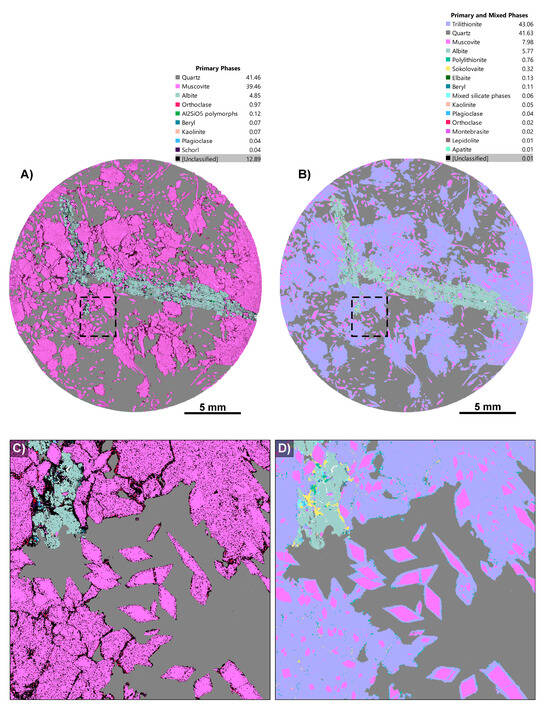
Figure 1.
Before and after phase maps for an LCT pegmatite sample, CS3.1. (A) “Before” phase map with the inbuilt Tescan classification scheme; (B) the same map after our custom phase library has been applied; (C) enlargement of the “before” phase map showing faint zoning in muscovite, giving a clue that the phase needs to be investigated; (D) enlargement of the “after” phase map showing the detailed zoning of muscovite and trilithionite. Other phases have been identified, including sokolovaite and minor polylithionite (see legend).
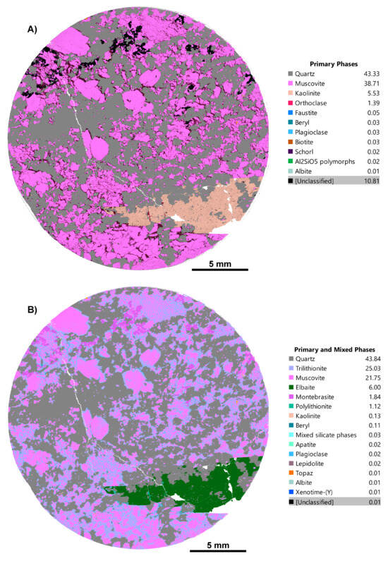
Figure 2.
Before (A,B) and after phase maps of an LCT pegmatite sample, CS3.3, showing the reduced unclassified phases (~10.8% down to 0.01%) and correct mineral identification, with kaolinite actually being a sodium tourmaline, elbaite.
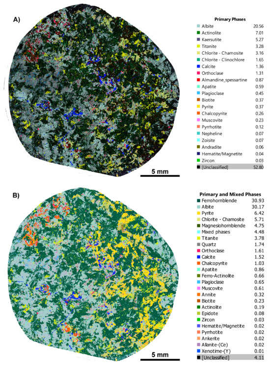
Figure 3.
Before and after phase maps for an IOCG deposit sample, CS1.1. (A) Before map with the in-built TIMA classification scheme showing 52.8% unclassified phases; (B) after map with our custom phase library, showing correct phase assignment and that the unclassified phases are down to 4%.
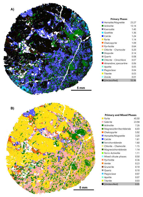
Figure 4.
(A) Before and (B) after phase maps for an IOCG deposit sample, CS1.2. (A) Phase map generated using the in-built TIMA classification scheme, with hematite/magnetite being the dominant phase and a high volume of unclassified phases (55.96%) present; (B) TIMA phase map of the same sample using our refined, deposit-specific, custom classification scheme for the IOCG sample. Now, phases are more correctly classified; for example, phases like pyrite (45.5%) and siderite (23.94%) are now recognised, and unclassified phases are down to 0.05%.
3.1. Unambiguous Characterisation of Major Rock-Forming Minerals
This case study comes from a North West Queensland iron–oxide–copper–gold (IOCG) deposit and involves common rock-forming minerals hosted in metasedimentary and volcanic host rocks; in this case, an albite +/− actinolite altered dolerite. The initial phase map was of poor quality, with 52.8% of pixels “unidentified” (Figure 3A). A major mineral in some samples showed prismatic habits with rhombic cross-sections and was clearly an amphibole. However, pixels were variously identified as “actinolite” or as the much more aluminous, high-Ti species kaersutite. Furthermore, some amphibole pixels were misidentified as almandine–spessartine garnet, a possibility that is discussed further below. These three phases made up only 13.2% of the map, although visually, the true total percentage of amphibole was much higher, implying that much of it remained “unclassified”. Careful examination of BSE and X-ray images revealed that the amphibole did indeed vary in composition within single crystals, but the then-current TIMA rules for common amphibole species did not accurately match the measured compositions. After several iterations of adjusting the rules for various mineral species, the improved phase map of Figure 3B was obtained. In this map, only 4.1% of pixels remain unclassified. The amphibole species identified are ferro-hornblende (30.93%), magnesio-hornblende (4.75%), ferro-actinolite (0.66%), and actinolite (0.19%), totalling 36.53% of the whole map. While not necessarily correct identifications, these are much closer to the actual situation, as ascertained by quantitative EPMA analysis of the selected points (Supplementary File S2, Table S2.2). The improbable high-Ti species and garnet are no longer identified. Furthermore, a change to the rules for albite also eliminated the unlikely phase nepheline (cf. example 2, above).
Early phase maps for this suite of rocks also required adjustment of TIMA identification criteria for sulphide minerals, the phases of principal economic interest. Figure 4 shows “before” and “after” refinement maps for a sulphide-rich sample in which much of the pyrite and chalcopyrite were not initially detected. Figure 5 illustrates a coincident bright BSE signal from sulphides and a strong sulphur signal in a multi-element map, indicating the presence of unidentified sulphide species. This prompted targeted refinement of the phase rules to resolve the misclassification (Figure 4), where the dominant sulphides were identified as pyrite and chalcopyrite. Despite the common sulphides pyrite and chalcopyrite being in the in-built TIMA phase library, they were not detected due to the in-built phase library entries being based on reference and/or ideal spectra and phase rules. Examination of this dataset further revealed that an abundant iron-rich matrix phase, originally identified as “hematite/magnetite” oxides (Figure 4A), was in fact the carbonate siderite (Figure 4B), distinguishable by its enhanced carbon and calcium peaks.
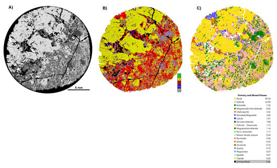
Figure 5.
Results from TIMA analysis for an IOCG deposit sample, CS1.2, showing an overview of maps used in our workflow. (A) BSE map; (B) multi-element map of standard elements used in determining phases; (C) final phase map.
In order to determine amphibole speciation, it should be noted that multiple single-site and coupled substitutions occur in the amphibole supergroup of minerals [47]. Species are defined by the predominant element of particular ionic charge(s) in each of four different types of cation sites (one very large “A” site that is often vacant, two large “B” sites that are often Ca, five octahedrally coordinated “C” sites that contain a wide range of possible elements, and eight tetrahedral “T” sites) and one anion site (not part of the [T8O22] double-chain anion, usually hydroxide), and the wide range of combinations available has resulted in the discovery and definition of over 140 amphibole species to date, although only a relatively small number of them are common.
A common type of compositional variation in Ca-rich amphiboles has some Al content introduced via the Tschermak substitution of Al3+Al3+ (on two different crystal structure sites) for M2+Si4+ of actinolite (M = Mg, Fe) to provide a “hornblende” amphibole. The prototypic magnesio-hornblende species is ideally Ca2(MgAl)(AlSi7O22)(OH)2. However, solid solutions can operate to provide other closely related possibilities:
- Fe2+ substituting for Mg in the octahedrally coordinated “C” sites. If Fe2+ > Mg, we have ferro-hornblende, ideally Ca2(Fe2+Al)(AlSi7O22)(OH)2.
- Fe3+ substituting for Al in the octahedrally coordinated “C” sites. If Fe3+ > Al, we have ferri-hornblende, ideally Ca2(MgFe3+)(AlSi7O22)(OH)2.
- Both “ferro-” and “ferri-” substitutions can operate to provide ferro-ferri-hornblende, Ca2(Fe2+Fe3+)(AlSi7O22)(OH)2.
- Additional Tschermak substitution can occur to provide tschermakite, Ca2(Mg3Al2)(Al2Si6O22)(OH)2, and its ferro- and ferri-analogues.
For the purposes of the current example, we will acknowledge but not discuss further additional variations, such as the incorporation of Na (a composition then tending towards edenite, pargasite/hastingsite, richterite, or winchite end-members) or Ti (a composition veering towards kaersutite).
Figure 6 shows different visualisations of the same small area of sample CS1.2, using the field view within the TIMA software, including a large and well-formed amphibole crystal. The BSE image shows an obvious dark core and bright rim, with hints of additional subtler zonation, including a very bright and thin outer rim. The X-ray heatmaps for Fe K and Mg K confirm that complementary variation in these elements in solid solutions is the main cause of the variation in BSE contrast. The BSE image allowed targeted EDS spectra to be obtained from small areas within each perceived zone and quantified in terms of atomic% element (excluding O and H; Figure 6F). Recalculation of the formulae then allowed for the provisional allocation of a species name to each analysis (see Supplementary File S1). The TIMA rules based on Al content and the Mg:Fe ratio were adjusted to distinguish the zones with sharp boundaries: relatively Fe-poor, Al-poor “actinolite” in the partly resorbed cores; Fe-rich, Al-rich “magnesio-ferri-hornblende”; and a thin rim of Fe-rich, Al-poor “ferro-actinolite”. Minor instances of “magnesio-hornblende” and “ferro-hornblende” were also observed in other grains scattered throughout the phase map.
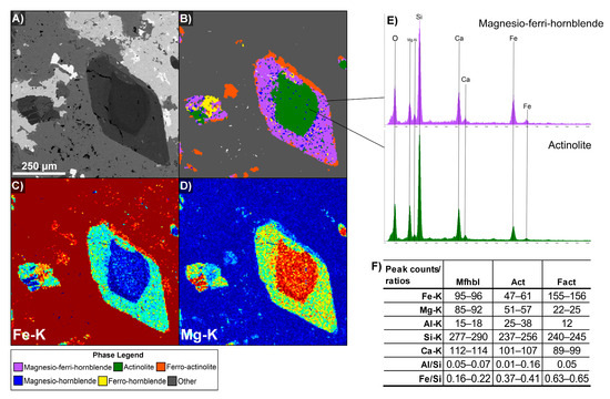
Figure 6.
Amphibole phase refinement based on a distinctive rhomb cross-section with at least three different BSE levels indicating elemental and phase variation. (A) BSE map of the amphibole rhomb. (B) The phase map has been recoloured for illustrative purposes to emphasise the zoning in the amphibole rhomb cross-section; see phase legend for mineral identification. (C,D) Element heatmaps for Fe K and Mg K, which were used for phase refinement. (E) shows the subtle visual difference between two EDS spectra for two of the three dominant amphibole composition zones examined; note that element peaks are all for K-families. (F) Numerical peak count and ratio ranges for the three dominant amphibole species in this field. Each image is 800 µm wide. Mineral abbreviations: Mfhbl = magnesio-ferri-hornblende, Act = actinolite, Fact = ferro-actinolite. Phase legend is in the bottom left corner of the figure.
Electron probe microanalysis (EPMA) was used to confirm the major- and minor-element concentrations of the amphiboles using a JEOL JXA-8530F field-emission microprobe at CARF QUT. Operating conditions included a 3 µm defocused beam, an accelerating voltage of 15 kV, and a beam current of 20 nA; further details of the analytical parameters and results are presented in Supplementary Files S1 and S2. Well-formed amphibole prismatic sections and rhomb cross-sections were targeted, as shown in Figure 7, from sample CS1.2. Scatter plots of wt% Mg vs. Fe and Al vs. Fe confirm that there are two separate amphibole populations (Figure 8A,B). Core compositions have high Mg (10.6–11.9 wt%) and restricted low ranges of Al (0.5–1.4 wt%) and Fe (5.6%–8.2%). A wide gap separates these from rim amphiboles, which have high Fe (11.6%–13.8%) and a range of Al, from a maximum 1.97% in the inner rim to a minimum 0.49% in the outer rim. Careful recalculation shows that these variations may not be quite extreme enough to reach the IMA-defined ferro-actinolite and magnesio-ferri-hornblende fields; instead, they are classified as distinct varieties of “actinolite” (Figure 8C). However, the clustering and trends are marked enough that provisional names have been retained for convenience. A non-standard colour scheme is used in the phase map of Figure 6B to highlight the zones. This sequence is unusual and scientifically important since it appears to document a complex history of prograde growth, resorption, regrowth, and retrogression. Amphiboles from the sample in Figure 4 are phase-mapped using the updated TIMA rules in Figure 7. A zonation pattern is also seen in BSE and X-ray maps (e.g., Figure 7), with the additional detail that there is a slight iron enrichment visible in the centres of the actinolite cores.
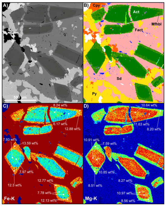
Figure 7.
A selected region from sample CS1.2, shown in Figure 5, where multiple EMPA measurements were taken. (A) BSE map showing the prismatic habit and rhombic cross-sections of the amphibole; BSE level changes from core to rim indicate element changes. (B) TIMA phase map after refinement of phases. (C,D) Magnesium and iron heatmaps show that the amphiboles have Mg cores and Fe rims, highlighting chemical zoning and likely phase changes. Upon refinement, there are at least three amphibole species, as shown in (B). Mineral abbreviations: Act = actinolite, Cpy = chalcopyrite, Fact = ferro-actinolite, Mfhbl = magnesio-ferri-hornblende, Py = pyrite, Sid = siderite. The phase legend in Figure 5C applies here. The scale bar in (A) applies to all images. Note: See Supplementary File S1, Figure S2, for a figure with EPMA analytical points and EPMA analytical parameters; summary EPMA results are in Supplementary File S2.
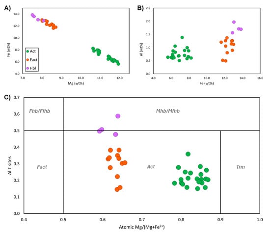
Figure 8.
Scatterplots of EPMA data from amphiboles in sample CS1.2. (A) Scatterplot of raw total wt% Mg versus Fe. Legend in (A) applies to all. (B) Raw wt% of Al against Fe wt%. (C) Amphibole Mg ratio versus tetrahedral Al. In each plot, it is apparent that there are two distinct populations of amphiboles. Data have been colour-coded to the assigned phase from the zoned amphibole rhomb in Figure 6, further highlighting that there are three populations, representing actinolite (Act), ferro-actinolite (Fact), and hornblende (Hbl). While the data for ferro-actinolite and some hornblendes still plot within the actinolite field in (C), provisional names are retained, as they are a distinct variety of actinolite; this is further explained in text. Note: Bulk data from all areas analysed, including unpublished data, are presented here. See Supplementary File S2, Table S2.1, for summary EPMA data.
A potential ambiguity that was discovered in the early stages of refining these phase maps was that parts of the amphibole grains were identified not as amphiboles but as almandine-rich garnet. The mineral texture observed in the phase map did not give any evidence for discrete garnet crystals, so this was clearly a suspect identification. It was deduced to arise as follows. While almandine garnet has the ideal formula Fe2+3Al2Si3O12, the Fe content can be partly replaced by substantial quantities of other divalent cations, Mg, Ca, or Mn, and the Al can be partly replaced by Fe3+. The mean charge of the cations in an anhydrous garnet is always +3 (yielding an 8:12 cation–oxygen ratio in the formula unit that is usually chosen). In an amphibole free of additional large cations (Na, K), whose 15 cations per formula unit have a total charge of +46, the mean cation charge is +46/15 = +3.067, which is clearly very similar to that of garnet. Given that an empirical formula derived from quantified EDS spectra contains no absolute information on O or H concentrations or Fe valence, just the atomic ratios of the other major and minor elements, it can be seen, in principle, that the relative ratios of Ca:Fe:Al:Si in a garnet and an amphibole might appear to be very similar. In fact, it is possible to construct hypothetical amphibole compositions whose Si content is 3/8 of the cation total, identical to that of a garnet. A worked example is shown in Supplementary File S1.
This case study illustrates the utility of TIMA in the study of rock-forming minerals with complex solid solutions that are potentially important thermobarometers and indicator minerals for metamorphic grade. Misidentifications (e.g., garnet for amphibole) can be identified by checking crystal habits, through knowledge of the petrogenetic context of the sample, and through examination of EDS data. In conjunction with BSE and EDS data, composition zones can be visualised and TIMA rules adjusted so that the zones can be mapped. However, more quantitative analytical data from EPMA may still be required for correct identification. This case highlights how mineralogical understanding and user knowledge of the sample and deposit can guide automated mineralogy, supported by geochemical and textural insights to refine phase assignments.
3.2. Identification and Deportment of Critical Elements
Copper, cobalt, arsenic, and bismuth are recognised as critical or strategic elements due to their essential roles in energy storage systems, electronics, and advanced manufacturing. In sediment-hosted polymetallic systems, these elements often occur as micron-scale inclusions or fine-grained discrete phases, posing challenges for accurate identification and mineral processing. Preliminary whole-rock geochemistry from a sediment-hosted Cu–Au–Co deposit in Queensland’s North West Minerals Province indicated significant Co (up to 2000 ppm) and Bi (over 1000 ppm) concentrations [48,49,50]. Further examination using micro-XRF revealed the presence of significant amounts of cobalt in tiny grains disseminated in a very fine laminated sedimentary rock, as well as in large crystals of pyrite and veins of copper-bearing sulphide phases. Cobalt substitutes readily for iron in pyrite [51,52]; however, there were clearly other microminerals present in which cobalt was the dominant cation. Thus, the TIMA was applied to investigate cobalt deportment within this deposit. High-resolution settings were used to explore the presence and distribution of fine-grained cobalt-bearing minerals within the samples, as well as to investigate the potential occurrence of cobalt in pyrite.
Discrete cobalt-dominant phases and other rare mineral phases were identified and added to the TIMA library. The high-resolution acquisition settings implemented allowed us to locate fine-grained phases, particularly cobalt-bearing phases, such as cobaltite (CoAsS). Figure 9 shows a heatmap of Co K, locating carrollite (CuCo2S4) and cobaltite within a sample, as indicated in the corresponding TIMA phase map (Figure 9B). The identification of phases was subsequently validated using EPMA (Tables S2.3a,b).
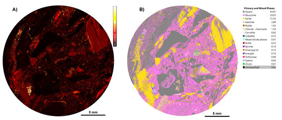
Figure 9.
TIMA maps for a Cu–Au–Co sample, CS2.1. (A) Co K heatmap showing distribution and intensity of Co K present in sample CS2.1; (B) phase map generated for sample CS2.1 using a custom, deposit-specific phase library from a sediment-hosted Cu–Au–Co deposit.
A particular issue with mapping cobalt is that Co immediately follows Fe in the Periodic Table, so the Co Kα X-rays (6.93 keV) are very close in energy to Fe Kβ X-rays (7.06 keV). Therefore, there is potential for interference from Fe in the “cobalt” element map obtained using Co K X-rays. A possible solution is to use the weaker Co Kβ characteristic X-rays (7.65 keV), which do not experience interference from Fe. These are close to Ni Kα at 7.48 keV and, hence, can be mapped using the “Ni K” energy window as a proxy. If the rock is poor in Ni, as in this case, most of the observed signal in that energy window should correspond to Co. Low-energy Co L (0.79–0.87 keV) could also be used, although, again, there is scope for overlap with adjacent elements and fluorine. This is one of many examples where energy windows for mapping may need to be chosen carefully because of the overlap between characteristic X-rays of common elements with those of less abundant elements of interest.
In order to check for the effects of overlap, we compared element maps obtained for a small region of the sample in Figure 10, using Fe K, Co K, Ni K, and Co L energy windows (see Supplementary File S1, Figure S3, for cumulative EDS spectra). The Co K signal is quite low in the large Fe-rich pyrite grains, implying little interference from Fe Kβ in practice. The Co K and Co L maps agree with each other well, while the Ni K map also seems to correlate strongly with them. Cobalt was also mapped independently using LA-ICPMS (see Supplementary File S1, Figure S4), which supported the X-ray maps used here. The variational behaviour of signals from the Fe K, Ni K, and Co K energy windows was investigated further, as follows. Greyscale images of the three maps were stacked together to make a composite red–green–blue image using the National Institute of Health ImageJ image-processing software (version 1.54p) (Figure 11A). Such an image allows the independent and covariational behaviour of the three signals to be visualised directly through changes in the resultant hue. Pyrite grains stand out in red, while Co phases are greenish-blue since Co Kα contributes strongly to the blue channel, while Co Kβ shows up mainly in the green channel. The signal from Ni Kα causes the colour to become even greener. The observation of bright green rims around grains in the image suggests that some genuinely Ni-rich phases exist, but only as these rims, which are too thin to analyse further. The ImageJ extension Fiji further allowed the intensity data from each greyscale image to be exported in spreadsheet form, allowing the co-variation of one energy window against another at the same pixel to be studied. The plot of Fe K versus Co K shows that they are quite independent (Figure 11B). Any combination of the two is possible, depending on whether X-rays are detected from pyrite, from a Co mineral, or from a grain boundary where interaction volumes overlap. However, a quite different trend is seen for Ni K versus Co K (Figure 11C). The linear positive correlation between the two shows the extent of Co Kβ interference in the Ni K signal, with the result that “Ni K” maps largely show the cobalt distribution in these samples. Points above the trend line are presumably from the Ni-rich “thin green rims” in the RGB image. This experiment demonstrated that the EDS energy windows used by TIMA can unambiguously map cobalt in the presence of minor Ni. Cobalt minerals that were located in element maps and then identified by EDS and EPMA included cobaltite (CoAsS), carrollite (CuCo2S4), and a Co arsenide phase (Supplementary File S2, Tables S2.3a and S2.3b). The latter mineral was present only as very fine grains that were only detected due to the use of high-resolution TIMA acquisition settings.
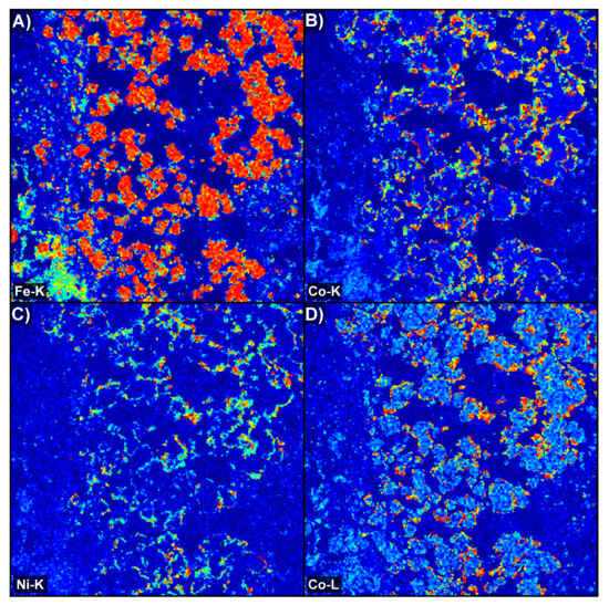
Figure 10.
Four-view grid showing TIMA EDS heatmaps representing intensity of (A) Fe K; (B) Co K; (C) Ni K; and (D) Co L. Here, it can be seen that the Co K signal is representative of the Co-bearing rims (in this case, cobaltite), while Fe K is restricted to the cores (pyrite), and no strong overlap is apparent. Co L weakly shows a signal in the Fe-rich cores, likely reflecting partial overlap between the Fe Lα and Co Lα X-rays, and the high Co L intensity on the rims corresponds to the Co K map. Interestingly, Ni K does show a signal on the cobalt rims, but without the same signal intensity. Each image is 800 µm wide. See Supplementary File S1, Figure S3, for details on the corresponding cumulative EDS spectra from this field and for all cobaltite in sample CS2.1, showing that while peaks for the α and β X-ray lines are indicated, they are not used independently in peak identification. Element families (K, L, M) are the selectable units for spectral peak analysis in the TIMA.
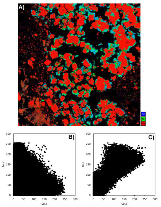
Figure 11.
(A) Composite RGB map using the element maps from Figure 10, where Fe K (red), Ni K (green), and Co K (blue) are layered (the image is 800 µm wide). (B,C) Scatterplots of the image intensity levels corresponding to normalised peak counts of the RGB channels to check for element interference. (B) Plot of cobalt versus iron (Co K vs. Fe K) and (C) plot of cobalt versus nickel (Ni K vs. Co K).
Element maps were also examined for other critical elements, such as Bi and Sb, in these samples, which led to the additional discovery of the Bi sulfosalt wittichenite (Cu3BiS3) and Cu–Sb–As sulfosalts. EPMA was again used to obtain accurate quantitative analyses, check mineral identifications, and provide further elemental information to refine the TIMA rules. The greater accuracy of EPMA over EDS was essential for the identification of the Co arsenide as safflorite, CoAs2, rather than the initial provisional identification as langisite (CoAs), and the As-rich sulfosalt as tennantite (Cu10M2+2As4S13) rather than enargite (Cu3AsS4). As a result of the latter identification, the two Cu–Sb–As sulfosalt phases were found to be both members of the “fahlerz” group (also known as the fahlore group), mainly tetrahedrite-(Zn) and tennantite-(Fe)—ideally, Cu10Zn2Sb4S13 and Cu10Fe2As4S13, respectively—with some zonation of the latter to tennantite-(Zn) [53]. The coexistence of two isostructural phases with an apparent solvus gap and coupling between Zn-Fe and Sb-As substitutions suggests that these minerals may have potential as thermobarometric indicators [54,55]. Refer to Supplementary File S2 for EPMA acquisition parameters and major element results. Figure 12 shows BSE images of the fine-grained sulphide and sulfosalt minerals of this study, as located by the TIMA and identified by EPMA.
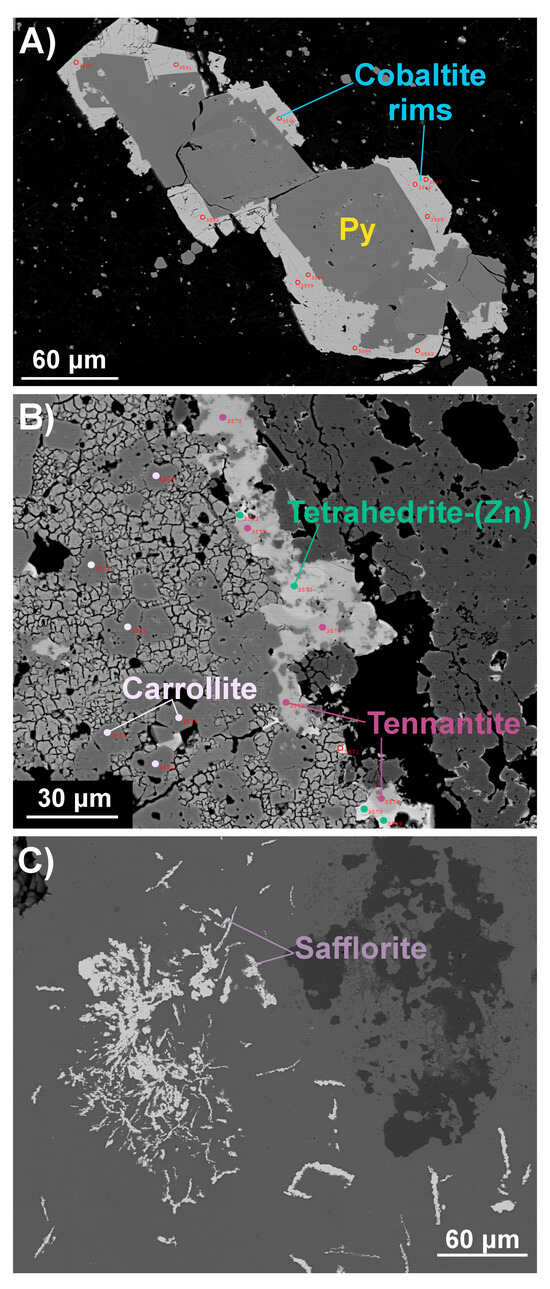
Figure 12.
Representative BSE images from EPMA analyses of fine-grained phases containing critical elements, including Co, Bi, and As. (A) Cobaltite rims around pyrite; (B) analysis points for carrollite, tetrahedrite-(Zn), and tennantite (Zn and Fe species); (C) safflorite displaying fine, fibrous morphology. All phase labels are coloured according to the custom TIMA phase library colour scheme. Note: See Supplementary File S2 for summary EPMA results.
Case study 2 demonstrates the power of high-resolution acquisition parameters used in our routine TIMA analyses to locate and map very fine-grained phases containing cobalt and other critical elements. Element maps can not only locate phases containing an element whose presence is known from other techniques (e.g., Co from µXRF data), but can also be used to check for the presence of hitherto unexpected critical elements of interest (e.g., Bi). While some EDS signal overlap may occur for some commonly associated elements (shown for Co Kβ in the Ni K data), it may not be important in practice (Fe Kβ in the Co K data) and can often be minimised by using mapping proxies (Co L and Ni K). Element mapping is a quick way to scan for and identify concentrations of such elements, which may result in the identification of scarce or microscopic and unusual phases, such as safflorite, wittichenite, and the tetrahedrite–tennantite of this study, which may otherwise escape notice. Again, it is noted that the use of EPMA for points of interest is an important adjunct technique to correctly identify such minerals, as EDS alone may not be sufficiently accurate. Other techniques, such as LA-ICPMS, may also supply valuable supporting data.
3.3. Indirect Identification of Diagnostic Light Elements
Lithium is a critical element with expanding industrial importance and increasing demand given the global energy transition. Globally, lithium is primarily mined from two major deposit types: salts (lithium-rich brines in salt lakes) and lithium minerals derived from granitic pegmatites [56]. In Australia, all current lithium resources and production are derived from hard-rock sources, especially lithium–caesium–tantalum (LCT) pegmatites, where the key lithium minerals include spodumene, petalite, and Li-bearing micas (lepidolite and zinnwaldite) [13,57]. As suggested by their name, such pegmatites also concentrate other critical elements, including the heavy alkali metals caesium and rubidium, along with elements such as beryllium and tantalum.
Lithium minerals are particularly challenging to characterise, as lithium (atomic number Z = 3) has characteristic X-rays that are extremely low energy (Li K = 0.055 keV) and thus are poor in yield relative to Auger electrons, strongly absorbed by all media, and unable to be detected by conventional SEM detectors. The situation is further complicated for Li micas by their extensive solid solution behaviour and similar major element compositions to Li-free or Li-poor related species. Nevertheless, accurate mineralogical characterisation of these systems is essential for understanding critical element deportment, resource evaluation, and downstream processing requirements. Automated mineralogy (AM) systems such as the TIMA offer a high-throughput method for mapping Li-bearing phases, but because SEM-EDS systems cannot measure light elements [6], indirect methods must be used to infer the presence of lithium.
Lithium-rich micas are generally trioctahedral, forming solid solutions that are called “lepidolite” when Al-rich and “zinnwaldite” when Fe-rich [58,59,60]. The principal IMA-defined “lepidolite” species are trilithionite, ideally K(Li1.5Al1.5)(AlSi3O10)F2, and polylithionite, K(Li2Al)(Si4O10)F2, while “zinnwaldite” is a solid solution between these and the “biotite” species annite and siderophyllite, KFe2+3(AlSi3O10)(OH)2—K(Fe2+Al)(Al2Si2O10)(OH)2. The substitution OH–F can be extensive in all of these micas, but it is not considered further in this contribution since it has no direct bearing on the Li content. In the LCT pegmatites considered here, primary spodumene and amblygonite are altered to produce Li-rich micas that intergrow with the Li-free dioctahedral mica muscovite, KAl2(AlSi3O10)(OH)2. The situation is further complicated by the discovery of luanshiweiite, an intermediate dioctahedral–trioctahedral mica that is compositionally halfway between muscovite and polylithionite, with the formula K(LiAl1.5)(Al0.5Si3.5O10)(OH)2 [61].
The Li+ cation is distinctive in its combination of low geochemical abundance, high lithophilicity, low charge, and moderate size (similar to Mg and Al), so it tends to concentrate in highly evolved pegmatitic fluids, where it most commonly first crystallises as the unusual pyroxene spodumene (LiAlSi2O6), the phosphate amblygonite (LiAlPO4), or as a range of Li-rich mica minerals, e.g., [62]. Here, we present results where the TIMA has successfully identified key mineral species within LCT pegmatite dyke samples, including differentiation of two different “lepidolite” populations corresponding to polylithionite and trilithionite, as well as the discovery of sokolovaite, a Cs-dominant analogue of polylithionite, in the sample suite. While the main chemical feature of interest, the lithium content, cannot be measured directly, it can be studied indirectly through its effect on the ratios of the charge-balancing Al and Si cations. Consider the atomic ratios K:Al:Si for the following end-member compositions in Table 1 and the ratio plot in Figure 13.

Table 1.
Atoms per formula units (a.p.f.u.) for primary cations detectable in EDS for mica end members. All numbers of atoms here correspond to a formula for the ideal end-member of the mica species, with 4 tetrahedral atoms per formula unit [46,63].
Figure 13.
Plot of atomic K/Al vs. Al/Si ratios for end-member mica groups in LCT pegmatites. Mineral abbreviations: Pln = polylithionite, Ann = annite, Sid = siderophyllite, Ms = muscovite, Tln = trilithionite, Lsw = luanshiweiite.
The Al:Si ratio inversely correlates with Li content across the trilithionite–polylithionite series due to Li substituting for Al in octahedral sites and associated Si enrichment in tetrahedral layers [58,64,65]. In contrast, Li substitution in lithian muscovite occurs via replacement of K, often reaching up to 1.5 wt% Li [13,65]. These substitution mechanisms informed the design of phase classification rules for the TIMA LCT pegmatite library, which were tuned using observed Al, Si, K, Cs, and Fe variation. Rule thresholds and ratio constraints were refined iteratively through phase map feedback, element map, and textural correlation, following the approach outlined in Section 2.3.3.
During the TIMA phase library-building process for the LCT pegmatite sample suite, aluminium heatmaps were particularly useful for visualising compositional distribution and zoning within mica grains (Figure 14). In sample CS3.1, a prismatic phase with rhombic cross-sections was initially classified as muscovite, but distinct zoning patterns were observed in the Al content (Figure 14A). Inspection of the EDS spectra from the Al-rich cores and Al-depleted rims showed clear changes in the Al, K, and Si count rates. These were able to be used to distinguish Al-rich muscovite in the cores from trilithionite rims that had decreased Al (Figure 1 and Figure 14B). In some regions of sample CS3.1, the Li-rich lepidolite end-member polylithionite was detected based on its characteristic very low Al and high Si content; it appeared in greater abundance elsewhere in the sample suite. Raman spectroscopy supported the presence of muscovite and trilithionite within sample CS3.1. To validate the inferred Li content and, hence, the phase assignments, LA-ICPMS area mapping was conducted on the sample, which confirmed lithium enrichment in the trilithionite rims (Figure 15). For detailed LA-ICPMS instrumentation and methods discussed here, refer to Supplementary Files S1 and S3.
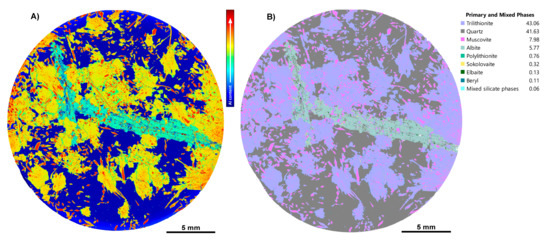
Figure 14.
Overview of LCT pegmatite sample CS3.1, which has been refined using Al, K, and Si to distinguish lepidolite species. (A) An aluminium heatmap highlighting zoning within rhombs and distribution throughout the sample; (B) TIMA phase map after a custom, deposit-specific phase library has been developed, capturing the distribution of trilithionite throughout the sample, including as rims around muscovite cores within pseudomorphed rhombs.
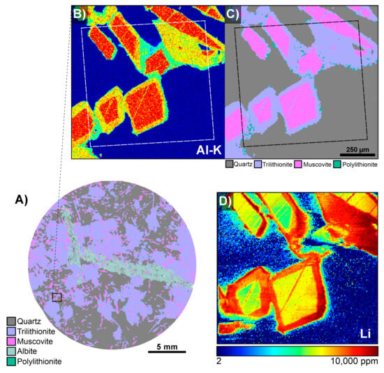
Figure 15.
(A) The overall TIMA phase map for LCT pegmatite sample CS3.1 showing the target map area; the black dashed box indicates where B and C are from. (B) A TIMA Al K heatmap showing the Al-rich cores of the rhombs and depleted rims. (C) Enlarged phase map showing the muscovite cores with trilithionite rims. The dashed boxes in both B and C indicate the LA-ICPMS map region. (D) LA-ICPMS map showing the distribution of lithium through the rhombs, with enriched Li rims, supporting that the rims are trilithionite.
In LCT pegmatite sample CS3.2, compositional outliers were observed, where aluminium did not behave the same as in other regions identified as muscovite and lepidolite elsewhere. The EDS spectra over these regions showed peaks for Cs L X-rays. Caesium heatmaps clearly indicated that a distinct Cs-rich mica phase was present (Figure 16A), e.g., [66,67], and Rb- and Cs-dominant species are now known. Through interrogation of the EDS spectrum from these regions, it was found that the phase is a Cs-dominant analogue of polylithionite, sokolovaite (CsLi2Al(Si4O10)F2 [68]), a Cs-mica that appears to have been documented from only seven localities worldwide [42,43] and not previously in Australia (Figure 16B). The sokolovaite identification was supported through LA-ICPMS mapping (Figure 17), where the distribution of Al, Li, and Cs confirms the close association of muscovite, trilithionite, and sokolovaite. Through iterative refinement of phase classification rules and validation using LA-ICPMS, sokolovaite was confidently identified in the TIMA phase map. The identification of this rare phase again highlights the effectiveness of integrating microanalytical workflows, combining the fast reconnaissance and mapping ability of TIMA with other techniques to characterise previously unrecognised critical metal-bearing phases.
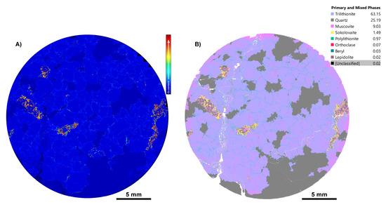
Figure 16.
Overview of LCT pegmatite sample CS3.2, which has been refined using Al, K, and Si to distinguish lepidolite species. In this sample, high levels of caesium were observed in concentrated regions of mica. (A) A cesium heatmap highlighting the intensity of Cs L, associated with mica; (B) TIMA phase map showing that the Cs-rich regions are in fact a Cs-mica, sokolovaite.
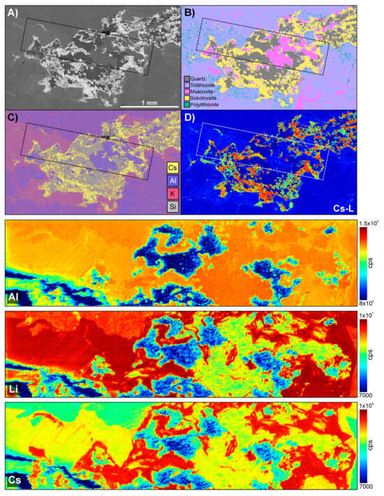
Figure 17.
Results for LA-ICPMS area mapping of a Cs-mica phase within LCT pegmatite sample CS3.2. (A–C) TIMA images from Figure 14 for LCT pegmatite sample CS3.2; (A) BSE image; (B) TIMA phase map; (C) multi-element map; (D) TIMA Cs L EDS heatmap. The dashed rectangle in each indicates the LA-ICPMS mapped region. The three images below are the LA-ICPMS maps for Al, Li, and Cs through the Cs-mica sokolovaite region. The Cs map shows that the distribution of Cs is strongest in regions identified as sokolovaite, supporting the TIMA findings.
To evaluate broader mica systematics and confirm the distinction between lepidolite species, LA-ICPMS spot analyses data from multiple samples and phases were examined. LA-ICPMS spot analyses (Supplementary File S3, Table S3.2) support the TIMA distinction between the Li/Si-rich and Li/Si-poor “lepidolite” species, polylithionite and trilithionite (Figure 18). Figure 18C shows a mica classification ternary diagram after Monier and Robert [69], highlighting that the species do not contain Fe and, hence, do not exhibit a solid solution towards zinnwaldite-type compositions. LA-ICPMS spot analyses directly confirm the contents of the critical element Li and, hence, the validity of TIMA mapping despite only being able to infer Li content indirectly.
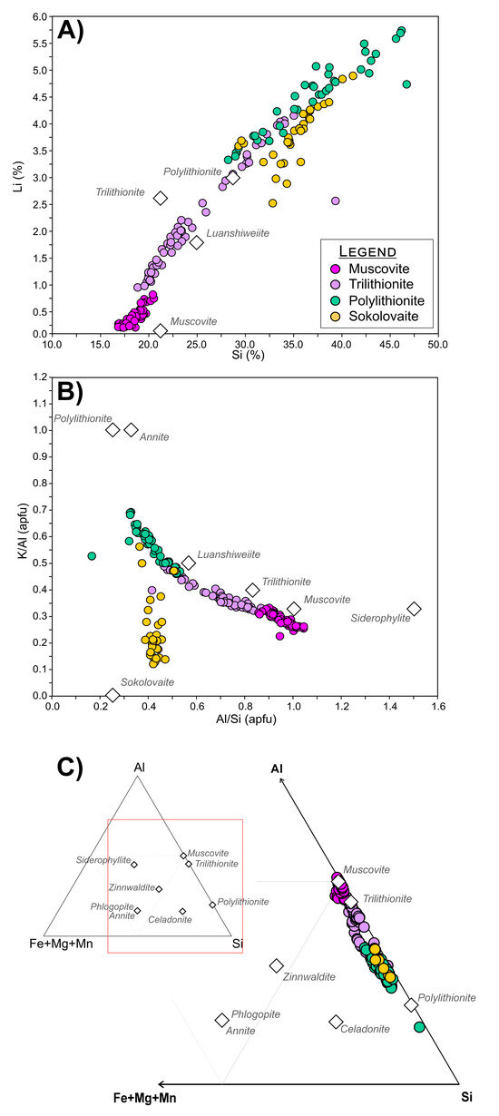
Figure 18.
Plots for mica phases from the LCT pegmatite samples using LA-ICPMS trace element spot analysis data. (A) Scatterplot of lithium (Li) versus silicon (Si) contents; (B) scatterplot of Si/Al versus K/Al ratios. Note that the diminished K/Al values of sokolovaite are due to Cs substitution for K in the mica lattice; (C) ternary diagram modified after Monier and Robert [69] of mica species classification, including trilithionite, polylithionite, and muscovite trace element spot data to show species groups with increased Li contents that correlate with Al and Si. Points are concentrated on the Al-Si axis and show a clear lack of Fe, Mg, and Mn expected in zinnwaldite-type mica compositions. Note: This plot contains unpublished data; examples of trace element LA-ICPMS spot data are presented in Supplementary Material File S3.
In addition to this suite of Li and Cs mica phases, these LCT pegmatites provided additional examples where minerals of light elements presented challenges for the TIMA. Through the processes outlined in Section 2.3 and Supplementary Materials File S1, the tourmaline-group species elbaite, Na(Li1.5Al1.5)Al6(Si6O18)(BO3)3(OH)3(OH), was also identified in the LCT pegmatites. Initially, this phase was classified as kaolinite, Al2(Si2O5)(OH)4 (Figure 2). However, through knowledge of the sample, this ~10 mm patch was known not to be a clay. Note that the atomic Al:Si ratios of elbaite and kaolinite are close, at 1.25:1 and 1:1, respectively. If only Al and Si counts are used to set TIMA rules, then elbaite is very likely to fit the criteria for kaolinite. Furthermore, the two most diagnostic elements in elbaite, Li and B, cannot be analysed by EDS. However, elbaite is a Na-rich tourmaline. The presence of sodium meant that elbaite could easily be distinguished from kaolinite once added to the phase library and with modification to the kaolinite rules. It should be noted that a greater challenge would have been presented by the alkali-free lithium tourmaline, rossmannite [70], ideally, □(LiAl2)Al6(Si6O18)(BO3)3(OH)3(OH) (where □ = vacant atomic site). In the absence of Na, the Al:Si ratio would be the only way for TIMA to distinguish rossmannite from kaolinite. The same is true of the beryllium mineral beryl, Al2Be3Si6O18, found in small amounts in this study but again only identifiable by its distinctive Al:Si ratio since beryllium cannot be identified directly in EDS.
This case study demonstrates the utility of automated mineralogy, supported by targeted microanalytical validation, for distinguishing Li-bearing micas and identifying unexpected rare phases like the Cs mineral sokolovaite within complex pegmatite systems. Through our process of iterative rule refinement, integrated element mapping, and cross-validation with complementary techniques like LA-ICPMS, we developed a reliable, deposit-specific classification scheme capable of resolving subtle compositional variations.
4. Conclusions
This paper demonstrates how targeted rule refinement and expert-guided phase library development can overcome key limitations in SEM-based automated mineralogy. Iterative refinement of deposit-specific TIMA phase libraries enables robust mineralogical characterisation of complex, compositionally variable mineral phases. By integrating high-resolution compositional, textural, and spectral data with validation from complementary techniques, including EPMA and LA-ICPMS, our approach improves classification in challenging mineral systems. Mineralogical understanding and user knowledge of the sample and deposit context are critical to addressing the inherent limitations of EDS-based classification and working within the constraints of AM software platforms such as TIMA.
We provide approaches for working both with and around the limitations of EDS and mineral chemistry, demonstrated through three detailed case studies from Queensland, Australia. In each, a deposit-specific phase library was iteratively developed in the TIMA: (1) refining amphibole classification in IOCG systems using compositional zoning, petrographic context, and EPMA data; (2) mapping fine-grained Co- and Bi-bearing phases in a sediment-hosted Cu–Au–Co deposit using high-resolution TIMA acquisition parameters, addressing EDS signal overlap, and revealing unexpected critical element phases, supported by EPMA and LA-ICPMS; and (3) indirectly identifying Li-mica species and the rare Cs-mica sokolvaite in a LCT pegmatite, using proxy element relationships validated through complementary LA-ICPMS analyses.
The case studies and examples presented here highlight that integrated microanalytical approaches are particularly effective for improved classification accuracy, reducing unclassified areas and revealing zoning, rare phases, and critical element-bearing phases. Application of these approaches improves deposit-specific mineral characterisation and supports more informed exploration strategies, as well as mineral deportment assessment for mineral processing. The lessons presented here are broadly applicable across automated mineralogy platforms and mineral systems research, offering a practical foundation for refining automated mineralogy approaches in both exploration and geoscience contexts.
Supplementary Materials
The following supporting information can be downloaded at https://www.mdpi.com/article/10.3390/min15111118/s1: Supplementary Material File S1 contains supplementary text information and figures. Figure S1. Standard TIMA measurement parameters. Figure S2. Expanded EPMA points for Figure 7, showing all amphibole EPMA measurement points collected in “Area 1”. Figure S3. Expanded version of Figure 10 showing the EDS spectra from the areas with the highest cobalt intensity. Figure S4. Case study 2: LA-ICPMS mapping results for Co-bearing phases. Supplementary Material File S2 contains Table S2.1 EPMA analytical parameters. Table S2.2. Summary table of major element results for case study 1 amphiboles. Table S2.3a. Summary table of major element results for case study 2 sulphides and arsenides. Table S2.3b. Summary table of major element results for case study 2 sulfosalts. Supplementary Material File S3 contains the following: Table S3.1. LA-ICPMS analytical parameters. Table S3.2. Spot analyses with trace element results for key micas from the LCT pegmatite samples. References [71,72,73] are found in Supplementary Materials.
Author Contributions
Conceptualisation, L.I.K., A.G.C., E.A.B., B.R.H. and A.K.-C.; methodology, L.I.K., E.A.B., M.d.B. and H.E.C.; software, not applicable; validation, L.I.K., A.G.C., E.A.B., B.R.H., A.K.-C., H.E.C. and M.d.B.; formal analysis, L.I.K., A.G.C., M.d.B., H.E.C., B.R.H. and E.A.B.; investigation, L.I.K., M.d.B., H.E.C., A.G.C. and E.A.B.; resources, V.L. and E.A.B.; data curation L.I.K. and E.A.B.; writing—original draft preparation, L.I.K. and A.G.C.; writing—review and editing, all authors; visualisation, L.I.K., A.G.C., E.A.B., B.R.H. and A.K.-C.; supervision, E.A.B., A.K.-C. and V.L.; project administration, L.I.K. and E.A.B.; funding acquisition, V.L. and E.A.B. All authors have read and agreed to the published version of the manuscript.
Funding
This project was funded by the Geological Survey of Queensland (GSQ) within the GSQ NEW Economy Minerals Initiative (NEMI) program and under the Umbrella Research Agreement with the Queensland University of Technology (NEMI-QUT-04 and NEMI-QUT-05).
Data Availability Statement
The original contributions presented in this study are included in the article and Supplementary Materials. Further inquiries can be directed to the corresponding authors. The raw data supporting this article will be made available by the authors upon request.
Acknowledgments
The data reported in this paper were obtained at the Central Analytical Research Facility (CARF) operated by Research Infrastructure at the Queensland University of Technology. The authors thank Charlotte M. Allen for discussions around manuscript conceptualisation and contents, draft editing, and support in access to facilities. The authors thank CARF staff for providing expertise and advice. We thank Rhiannon Jones for manuscript conceptualisation discussions. We also acknowledge the team at AXT Pty Ltd., the authorised vendor for Tescan instrumentation in Australia, for their technical support and training on the Tescan TIMA. The authors thank Zofia Swierczek for early guidance and assistance with the TIMA and for valuable discussions on phase library approaches and optimisation. We thank the reviewers and editors for their time and expertise in evaluating our work. The constructive comments of the four anonymous reviewers considerably contributed to the improvement of this manuscript.
Conflicts of Interest
The authors declare no conflicts of interest.
Abbreviations
The following abbreviations are used in this manuscript:
| AM | Automated mineralogy |
| TIMA | Tescan Integrated Mineral Analyzer |
| BSE | Back-scattered electron |
| EDS | Energy-dispersive X-ray spectroscopy |
| EPMA | Electron probe microanalysis |
| LA-ICPMS | Laser ablation inductively coupled plasma mass spectrometry |
| XRD | X-ray diffraction |
| IOCG | Iron–oxide–copper-gold |
| LCT | Lithium–caesium–tantalum |
| SEM | Scanning electron microscopy |
| MLA | Mineral Liberation Analyzer |
| CARF | Central Analytical Research Facility |
| QUT | Queensland University of Technology |
| FEG | Field emission gun |
| SE | Secondary electron |
| CL | Cathodoluminescence |
| BI | Beam intensity |
| WD | Working distance |
| ICR | Input count rate |
| IMA | International Mineralogical Association |
References
- Hrstka, T.; Gottlieb, P.; Skála, R.; Breiter, K.; Motl, D. Automated mineralogy and petrology—Applications of TESCAN Integrated Mineral Analyzer (TIMA). J. Geosci. 2018, 63, 47–63. [Google Scholar] [CrossRef]
- Miller, P.; Reid, A.; Zuiderwyk, M. QEM* SEM image analysis in the determination of modal assays, mineral associations and mineral liberation. In Proceedings of the XIV International Mineral Processing Congress: Worldwide Industrial Application of Mineral Processing Technology, Toronto, ON, Canada, 17–23 October 1982; pp. VIII-3.1–VIII-3.20. [Google Scholar]
- Reid, A.; Gottlieb, P.; MacDonald, K.; Miller, P. QEM* SEM image analysis of ore minerals: Volume fraction, liberation and observational variances. Appl. Mineral. 1984, 191–204. [Google Scholar]
- Fandrich, R.; Gu, Y.; Burrows, D.; Moeller, K. Modern SEM-based mineral liberation analysis. Int. J. Miner. Process. 2007, 84, 310–320. [Google Scholar] [CrossRef]
- Gu, Y. Automated scanning electron microscope based mineral liberation analysis. J. Miner. Mater. Charact. Eng. 2003, 2, 33–41. [Google Scholar] [CrossRef]
- Schulz, B.; Sandmann, D.; Gilbricht, S. SEM-based automated mineralogy and its application in geo-and material sciences. Minerals 2020, 10, 1004. [Google Scholar] [CrossRef]
- Gottlieb, P.; Wilkie, G.; Sutherland, D.; Ho-Tun, E.; Suthers, S.; Perera, K.; Jenkins, B.; Spencer, S.; Butcher, A.; Rayner, J. Using quantitative electron microscopy for process mineralogy applications. JOM 2000, 52, 24–25. [Google Scholar] [CrossRef]
- Hoal, K.; Stammer, J.; Appleby, S.; Botha, J.; Ross, J.; Botha, P. Research in quantitative mineralogy: Examples from diverse applications. Miner. Eng. 2009, 22, 402–408. [Google Scholar] [CrossRef]
- Baum, W. Ore characterization, process mineralogy and lab automation a roadmap for future mining. Miner. Eng. 2014, 60, 69–73. [Google Scholar] [CrossRef]
- Guhl, A.C.; Greb, V.-G.; Schulz, B.; Bertau, M. An improved evaluation strategy for ash analysis using scanning electron microscope automated mineralogy. Minerals 2020, 10, 484. [Google Scholar] [CrossRef]
- Schulz, B.; Merker, G.; Gutzmer, J. Automated SEM mineral liberation analysis (MLA) with generically labelled EDX spectra in the mineral processing of rare earth element ores. Minerals 2019, 9, 527. [Google Scholar] [CrossRef]
- Aylmore, M.G.; Eksteen, J.J.; Jones, M.G.; Wells, M. The mineralogy and processing potential of the Commonwealth project in the Molong Volcanic Belt, central eastern New South Wales, Australia. Ore Geol. Rev. 2019, 111, 102976. [Google Scholar] [CrossRef]
- Aylmore, M.G.; Merigot, K.; Quadir, Z.; Rickard, W.D.; Evans, N.J.; McDonald, B.J.; Catovic, E.; Spitalny, P. Applications of advanced analytical and mass spectrometry techniques to the characterisation of micaceous lithium-bearing ores. Miner. Eng. 2018, 116, 182–195. [Google Scholar] [CrossRef]
- Emo, R.B.; Kamber, B.S. A reconstitution approach for whole rock major and trace element compositions of granulites from the kapuskasing structural zone. Minerals 2020, 10, 573. [Google Scholar] [CrossRef]
- Emo, R.B.; Kamber, B.S. Evidence for highly refractory, heat producing element-depleted lower continental crust: Some implications for the formation and evolution of the continents. Chem. Geol. 2021, 580, 120389. [Google Scholar] [CrossRef]
- Holwell, D.A.; Adeyemi, Z.; Ward, L.A.; Smith, D.J.; Graham, S.D.; McDonald, I.; Smith, J.W. Low temperature alteration of magmatic Ni-Cu-PGE sulfides as a source for hydrothermal Ni and PGE ores: A quantitative approach using automated mineralogy. Ore Geol. Rev. 2017, 91, 718–740. [Google Scholar] [CrossRef]
- Kern, M.; Möckel, R.; Krause, J.; Teichmann, J.; Gutzmer, J. Calculating the deportment of a fine-grained and compositionally complex Sn skarn with a modified approach for automated mineralogy. Miner. Eng. 2018, 116, 213–225. [Google Scholar] [CrossRef]
- Keulen, N.; Malkki, S.N.; Graham, S. Automated quantitative mineralogy applied to metamorphic rocks. Minerals 2020, 10, 47. [Google Scholar] [CrossRef]
- Liu, T.; Song, W.; Kynicky, J.; Yang, J.; Chen, Q.; Tang, H. Automated quantitative characterization REE ore mineralogy from the giant Bayan Obo Deposit, Inner Mongolia, China. Minerals 2022, 12, 426. [Google Scholar] [CrossRef]
- Murphy, D.T.; Emo, R.; Deegan, B.; Allen, C. Growth and evolution of NE Australian continental crust interpreted from complex melting-hybridization histories of northern Queensland granulite xenoliths. Gondwana Res. 2023, 113, 163–178. [Google Scholar] [CrossRef]
- Perez-Barnuevo, L.; Pirard, E.; Castroviejo, R. Automated characterisation of intergrowth textures in mineral particles. A case study. Miner. Eng. 2013, 52, 136–142. [Google Scholar] [CrossRef]
- Rollinson, G.K.; Andersen, J.C.; Stickland, R.J.; Boni, M.; Fairhurst, R. Characterisation of non-sulphide zinc deposits using QEMSCAN®. Miner. Eng. 2011, 24, 778–787. [Google Scholar] [CrossRef]
- Santoro, L.; Putzolu, F.; Mondillo, N.; Herrington, R.; Najorka, J.; Boni, M.; Dosbaba, M.; Maczurad, M.; Balassone, G. Quantitative mineralogical evaluation of Ni-Co laterite ores through XRPD-QPA-and automated SEM-based approaches: The Wingellina (Western Australia) case study. J. Geochem. Explor. 2021, 223, 106695. [Google Scholar] [CrossRef]
- Schulz, B. Polymetamorphism in garnet micaschists of the Saualpe Eclogite Unit (Eastern Alps, Austria), resolved by automated SEM methods and EMP–Th–U–Pb monazite dating. J. Metamorph. Geol. 2017, 35, 141–163. [Google Scholar] [CrossRef]
- Shan, P.; Cao, M.; Evans, N.J.; Gao, H.; Mao, Y.; Gao, Y.; Salazar, L.; Zhao, Y.; Qin, K. Automated quantitative mineralogy analysis reveals characteristics of Co occurrence in the Jinchang porphyry deposit, NE China. Ore Geol. Rev. 2023, 158, 105524. [Google Scholar] [CrossRef]
- Taylor, R.J.; Hill, E.; Andrew, M. A step forward in quantitative automated mineralogy in 2D and 3D. Geostand. Geoanal. Res. 2024, 48, 579–593. [Google Scholar] [CrossRef]
- Yang, J.; Song, W.; Liu, Y.; Zhu, X.; Kynicky, J.; Chen, Q. Mineralogy and element geochemistry of the Bayan Obo (China) carbonatite dykes: Implications for REE mineralization. Ore Geol. Rev. 2024, 165, 105873. [Google Scholar] [CrossRef]
- Yu, X.; Su, X.; Wang, Z.; Hou, Z.; Li, B.; Deng, T.; Yan, Z. Genesis of the Xiangshan Uranium Ore Field: Implications from Tescan Integrated Mineral Analyzer and Micro-X-Ray Fluorescence Mapping and Thermodynamic Modeling. Minerals 2024, 15, 5. [Google Scholar] [CrossRef]
- da Silva, F.L.; Moreira, G.F.; Pires, K.S.; von Kruger, F.L.; da Silva Araujo, F.G. Quantitative phases characterization of clayey ceramics containing manganese ore tailings. J. Mater. Res. Technol. 2020, 9, 11884–11894. [Google Scholar] [CrossRef]
- Harvey, P.J.; Rouillon, M.; Dong, C.; Ettler, V.; Handley, H.K.; Taylor, M.P.; Tyson, E.; Tennant, P.; Telfer, V.; Trinh, R. Geochemical sources, forms and phases of soil contamination in an industrial city. Sci. Total Environ. 2017, 584, 505–514. [Google Scholar] [CrossRef]
- Hrstka, T.; Motl, D.; Gottlieb, P.; Hladil, J. Using an automated approach in building a dust particle atlas for research and environmental monitoring. Sci. Res. Abstr. 2017, 6, 43. [Google Scholar]
- Knappett, C.; Pirrie, D.; Power, M.R.; Nikolakopoulou, I.; Hilditch, J.; Rollinson, G.K. Mineralogical analysis and provenancing of ancient ceramics using automated SEM-EDS analysis (QEMSCAN®): A pilot study on LB I pottery from Akrotiri, Thera. J. Archaeol. Sci. 2011, 38, 219–232. [Google Scholar] [CrossRef]
- Kostryzhev, A.; Murphy, T. Phase characterisation in minerals and metals using an SEM-EDS based automated mineralogy system. Methods Microsc. 2025, 1, 163–175. [Google Scholar] [CrossRef]
- Crompton, J.W. Weathering products in glacial silt and clay: Using automated mineralogy to probe size distribution and source. Arct. Antarct. Alp. Res. 2025, 57, 2438462. [Google Scholar] [CrossRef]
- Figueroa, G.; Moeller, K.; Buhot, M.; Gloy, G.; Haberla, D. Advanced discrimination of hematite and magnetite by automated mineralogy. In Proceedings of the 10th International Congress for Applied Mineralogy (ICAM), Trondheim, Norway, 1–5 August 2011; pp. 197–204. [Google Scholar]
- Kearney, L.; Nothdurft, L.; Murphy, D.; Webb, G.E.; Webster, J. Characterising Microtextural and Mineralogical Features of Reef Rocks using Automated Mineral Analysis. In Proceedings of the 13th Asia Pacific Microscopy Congress 2025 (APMC13), Brisbane, Australia, 2–7 February 2025; p. 270. [Google Scholar]
- Swierczek, Z.; Quast, K.; Addai-Mensah, J.; Connor, J.N.; Li, J.; Robinson, D.J. Mineralogical characterisation of a sample of an Australian nickel laterite. In Proceedings of the Chemeca 2011: Engineering a Better World, Sydney, NSW, Australia, 18–21 September 2011; pp. 1755–1764. [Google Scholar]
- Weislogel, A.; Pfaff, K.; Knapp, J. Leveraging Automated Mineralogy Analysis to Assess Paleosol Chemical Weathering; Goldschmidt: Leipzig, Germany, 2025. [Google Scholar]
- Wilton, D.H.; Thompson, G.M.; Grant, D.C. The use of automated indicator mineral analysis in the search for mineralization—A next generation drift prospecting tool. Assoc. Appl. Geochem. Explor. Newsl. 2017, 174, 1–18. [Google Scholar] [CrossRef]
- Motl, D.; Filip, V. Method and Apparatus for Material Analysis by a Focused Electron Beam Using Characteristic X-Rays and Back-Scattered Electrons. US 13/398,114, 28 February 2013. [Google Scholar]
- Mineralogy Database. Available online: https://webmineral.com/ (accessed on 1 September 2025).
- Mindat. Available online: https://www.mindat.org/ (accessed on 1 September 2025).
- Ralph, J.; Von Bargen, D.; Martynov, P.; Zhang, J.; Que, X.; Prabhu, A.; Morrison, S.M.; Li, W.; Chen, W.; Ma, X. Mindat. org: The open access mineralogy database to accelerate data-intensive geoscience research. Am. Mineral. 2025, 110, 833–844. [Google Scholar] [CrossRef]
- Klein, C.; Dutrow, B. Manual of Mineral Science (After James D. Dana), 23rd ed.; John Wiley and Sons: Hoboken, NJ, USA, 2007. [Google Scholar]
- Putnis, A. Introduction to Mineral Sciences; Cambridge University Press: Cambridge, UK, 1992. [Google Scholar]
- International Mineralogical Association Commission for New Minerals, Nomenclature and Classification (2025) IMA-CNMNC List of Mineral Names (September 2025). Available online: https://cnmnc.units.it/index.php (accessed on 1 October 2025).
- Hawthorne, F.C.; Oberti, R.; Harlow, G.E.; Maresch, W.V.; Martin, R.F.; Schumacher, J.C.; Welch, M.D. Nomenclature of the amphibole supergroup. Am. Mineral. 2012, 97, 2031–2048. [Google Scholar] [CrossRef]
- Belousova, E.; Listin, V.; Dhnaram, C.; Blake, P.; Tang, J.; Gopalakrishnan, S.; Killen, D.; von Gnielinski, F.E.; Valetich, M. Hyperspectral imaging and whole-rock multi-element geochemistry for Pb-Zn-Ag and Cu deposits of NW Queensland—Data package. In GSQ Technical Notes 2022/04; Queensland Government: Brisbane, Australia, 2022. [Google Scholar]
- Evans, T. Chapter 23—Mount Oxide. In North West Mineral Province Deposit Atlas; Queensland Government: Brisbane, Australia, 2025; pp. 725–755. [Google Scholar]
- Valenta, R. NW Queensland Mineral Province Deposit Atlas Prototype Report–the Mount Isa and Ernest Henry Deposits. In DNRME-GSQ Commissioned Study and Report; The Sustainable Minerals Institute: Brisbane, Australia, 2018. [Google Scholar]
- Qiu, Z.-J.; Xing, Y.; Brugger, J.; Etschmann, B.; Pintér, Z.; Fougerouse, D.; Xu, J.; Yu, Z.; Guo, G.-J.; Fan, H.-R. Vacancies in sulfides facilitate fluid-induced solid-state diffusion and critical metals accumulation. Nat. Commun. 2025, 16, 1835. [Google Scholar] [CrossRef]
- Yaylali, B.; Deveci, H.; Yazici, E.Y.; Celep, O. Extraction of cobalt from a cobaltiferrous pyrite concentrate using H2SO4-NaNO3 lixiviant system. Miner. Eng. 2023, 198, 108077. [Google Scholar] [CrossRef]
- Sack, R.O. Fahlore thermochemistry: Gaps inside the (Cu, Ag) 10 (fe, zn) 2 (sb, as) 4S13 cube. Petrology 2017, 25, 498–515. [Google Scholar] [CrossRef]
- Sack, R.O.; Loucks, R.R. Thermodynamic properties of tetrahedrite-tennantite: Constraints on the interdependence of the Ag ⇌ Cu, Fe ⇌ Zn, Cu ⇌ Fe, and As ⇌ Sb exchange reactions. Am. Mineral. 1985, 70, 1270–1289. [Google Scholar]
- Dincă, G.; Popescu, G.C.; Topa, D. Decoding the mineralogy and geochemistry of sulfosalts in the Săcărâmb Au-Ag-Te ore deposit (Romania): Unveiling a fresh insight into the evolution of a complex hydrothermal system. Ore Geol. Rev. 2025, 176, 106424. [Google Scholar] [CrossRef]
- Kesler, S.E.; Gruber, P.W.; Medina, P.A.; Keoleian, G.A.; Everson, M.P.; Wallington, T.J. Global lithium resources: Relative importance of pegmatite, brine and other deposits. Ore Geol. Rev. 2012, 48, 55–69. [Google Scholar] [CrossRef]
- Britt, A.; Czarnota, K. A review of critical mineral resources in Australia. Aust. J. Earth Sci. 2024, 71, 1016–1049. [Google Scholar] [CrossRef]
- Foster, M.D. Interpretation of the Composition of Lithium Micas; United States Government Printing Office: Washington, DC, USA, 1960; pp. 2330–7102. [Google Scholar]
- Tischendorf, G.; Forster, H.-J.; Gottesmann, B.; Rieder, M. True and brittle micas: Composition and solid-solution series. Mineral. Mag. 2007, 71, 285–320. [Google Scholar] [CrossRef]
- Rieder, M.; Cavazzini, G.; D’yakonov, Y.S.; Frank-Kamenetskii, V.A.; Gottardi, G.; Guggenheim, S.; Koval, P.W.; Mueller, G.; Neiva, A.M.; Radoslovich, E.W. Nomenclature of the micas. Clays Clay Miner. 1998, 46, 586–595. [Google Scholar] [CrossRef]
- Fan, G.; Li, G.; Shen, G.; Xu, J.; Dai, J. Luanshiweiite: A new member of lepidolite series. Acta Mineral. Sin. 2013, 33, 713–721. [Google Scholar]
- Hines, B.; Turnbull, D.; Ashworth, L.; McKnight, S. Geochemical characteristics and structural setting of lithium–caesium–tantalum pegmatites of the Dorchap Dyke Swarm, northeast Victoria, Australia. Aust. J. Earth Sci. 2023, 70, 763–800. [Google Scholar] [CrossRef]
- IMA Database of Mineral Properties. Available online: https://rruff.info/ima/ (accessed on 1 October 2025).
- Brigatti, M.F.; Caprilli, E.; Malferrari, D.; Medici, L.; Poppi, L. Crystal structure and chemistry of trilithionite-2 M 2 and polylithionite-2 M 2. Eur. J. Mineral. 2005, 17, 475–481. [Google Scholar] [CrossRef]
- Brigatti, M.F.; Kile, D.E.; Poppi, M. Crystal structure and crystal chemistry of lithium-bearing muscovite-2 M 1. Can. Mineral. 2001, 39, 1171–1180. [Google Scholar] [CrossRef]
- Černý, P.; Chapman, R.; Teertstra, D.K.; Novák, M. Rubidium-and cesium-dominant micas in granitic pegmatites. Am. Mineral. 2003, 88, 1832–1835. [Google Scholar] [CrossRef]
- Wang, R.; Hu, H.; Zhang, A.; Fontan, F.; de Parseval, P.; Jiang, S. Cs-dominant polylithionite in the Koktokay# 3 pegmatite, Altai, NW China: In situ micro-characterization and implication for the storage of radioactive cesium. Contrib. Mineral. Petrol. 2007, 153, 355–367. [Google Scholar]
- Pautov, L.; Agakhanov, A.; Bekenova, G. Sokolovaite CsLi2AlSi4O10F2—A new mineral species of the mica group. New Data Miner. 2006, 41, 5–13. [Google Scholar]
- Monier, G.; Robert, J.-L. Evolution of the miscibility gap between muscovite and biotite solid solutions with increasing lithium content: An experimental study in the system K2O-Li2O-MgO-FeO-Al2O3-SiO2-H2O-HF at 600 °C, 2 kbar PH2O: Comparison with natural lithium micas. Mineral. Mag. 1986, 50, 641–651. [Google Scholar] [CrossRef]
- Selway, J.B.; Novak, M.; Hawthorne, F.C.; Cerny, P.; Ottolini, L.; Kyser, T.K. Rossmanite,[](LiAl2)Al6(Si6O18)(BO3)3(OH)4, a new alkali-deficient tourmaline; description and crystal structure. Am. Mineral. 1998, 83, 896–900. [Google Scholar] [CrossRef]
- Jochum, K.P.; Weis, U.; Stoll, B.; Kuzmin, D.; Yang, Q.; Raczek, I.; Jacob, D.E.; Stracke, A.; Birbaum, K.; Frick, D.A. Determination of reference values for NIST SRM 610–617 glasses following ISO guidelines. Geostand. Geoanal. Res. 2011, 35, 397–429. [Google Scholar] [CrossRef]
- Paton, C.; Hellstrom, J.; Paul, B.; Woodhead, J.; Hergt, J. Iolite: Freeware for the visualisation and processing of mass spectrometric data. J. Anal. At. Spectrom. 2011, 26, 2508–2518. [Google Scholar] [CrossRef]
- Jochum, K.P.; Willbold, M.; Raczek, I.; Stoll, B.; Herwig, K. Chemical Characterisation of the USGS Reference Glasses GSA-1G, GSC-1G, GSD-1G, GSE-1G, BCR-2G, BHVO-2G and BIR-1G Using EPMA, ID-TIMS, ID-ICP-MS and LA-ICP-MS. Geostand. Geoanal. Res. 2005, 29, 285–302. [Google Scholar] [CrossRef]
Disclaimer/Publisher’s Note: The statements, opinions and data contained in all publications are solely those of the individual author(s) and contributor(s) and not of MDPI and/or the editor(s). MDPI and/or the editor(s) disclaim responsibility for any injury to people or property resulting from any ideas, methods, instructions or products referred to in the content. |
© 2025 by the authors. Licensee MDPI, Basel, Switzerland. This article is an open access article distributed under the terms and conditions of the Creative Commons Attribution (CC BY) license (https://creativecommons.org/licenses/by/4.0/).