Fracture Density Prediction of Basement Metamorphic Rocks Using Gene Expression Programming

Abstract

Many methods have been developed to detect and predict the fracture properties of fractured rocks. The standard data sources for fracture evaluations are image logs and core samples. However, many wells do not have these data, especially for old wells. Furthermore, operating both methods can be costly, and, sometimes, the data gathered are of bad quality. Therefore, previous research attempted to evaluate fractures indirectly using the widely available conventional well-logs. Sedimentary rocks are widespread and have been studied in the literature. However, fractured reservoirs, like igneous and metamorphic rock bodies, may also be vital since they provide fluid migration pathways and can store some hydrocarbons. Hence, two fractured metamorphic rock bodies are studied in this study to evaluate any difference in fracture responses on well-log properties. Also, a quick and reliable prediction method is studied to predict fracture density (FD) in the case of the unavailability of image logs and core samples. Gene expression programming (GEP) was chosen for this study to predict FD, and ten conventional well-log data were used as input variables. The model produced by GEP was good, with R2 values at least above 0.84 for all studied wells, and the model was then applied to wells without image logs. Both selected metamorphic rocks showed similar results in which the significant parameters to predict FD were the spectral gamma ray, resistivity, and porosity logs. This study also proposed a validation method to ensure that the FD value predictions were consistent using discriminant function analysis. In conclusion, the GEP method is reliable and could be used for FD predictions for basement metamorphic rocks.

1. Introduction

Understanding fractured reservoir properties is crucial since they provide valuable information, especially when developing a reservoir model [1]. Fractures provide fluid flow in the reservoir and store a significant amount of fluid, be it water or hydrocarbon [2,3,4]. Interpreting fractured reservoir properties can be achieved using two approaches, which are direct and indirect methods [5]. Direct methods include evaluating and interpreting core samples (including analysing the outcrop samples and computed tomography scan of core samples) and image logs (electrical and acoustic) [6,7,8,9,10,11]. According to [12], these two approaches are probably the most essential to evaluate fractures since they have a higher resolution and a small margin of error, especially for depth conversion, when compared to the seismic method, but some studies also discussed the limitations of both methods [13,14,15,16]. Core samples are not always available, are expensive, and the retrieving process sometimes fails. Even if the coring process is successful, it often does not target the desired depth in which fractures are expected [4,6,13]. Another source of direct fracture information is image logs, which have been widely used in industry and studied in the literature [14,15]. Although image logs can efficiently point out the target depths for core retrieval [6], they are costly, and very few companies would opt for this option for every single well [16].

The indirect method of evaluating fractures comes from conventional well-logs: gamma ray or spectral gamma ray, porosity, and resistivity logs [17]. Many researchers utilise the widely available conventional well-logs since most wells have conventional well-log data, especially older wells. It has been agreed that the gamma ray log itself cannot indicate fractures effectively. However, spectral gamma ray information and potassium, uranium, and thorium logs help identify the presence of the initial fracture [18,19]. This is especially true in the case of uranium log readings. Fluid activity is more active in a fracture zone and will subsequently result in uranium mineral precipitation along the fractures due to the uranium characteristics of being readily soluble in both water and hydrocarbon [18,20]. Although high levels of uranium could also be caused by different factors and is not necessarily due to fractures, it is a good indirect indicator for initial fracture assessment [20]. This enrichment of uranium in the formation results in the abnormally high reading for uranium content in the well-logs [21]. Porosity logs could be beneficial when interpreting the fracture zones indirectly. Density logs are known for their ability to read the formation’s bulk density. When there are fractures, the density log readings will be lower. Hence, the well-logs will show a spike with low-density log readings. Besides the presence of hydrocarbon and coal seams, the existence of vugs and cavities will also give similar low readings in density logs [18].

Neutron logs are helpful when combined with density logs to show evidence of fracture in the well-logs, although it is not a primary use of these logs. Neutron logs are used to provide the apparent porosity values of the formation. When density and neutron logs are combined, a sharp decrease in the density log and a sharp increase in the neutron log can be interpreted as fracture existence [22]. Therefore, density and neutron logs should be used together to interpret the fracture even though there are several uncertainties and assumptions that have to be considered [19]. The sonic or acoustic log is another porosity log that helps to indicate a fracture. The sonic tool emits sound waves to the formation, and the tool records the travel time from the transmitter to the formation and back to the receiver on the tool. Depending on the fractures’ fillings and types, the fractures will eventually reduce the density of the formation; hence, a fractured zone reduces the sound wave transmission speed. This will result in sharp spikes in the interval transit time, and cycle skipping might occur on the log [16,17,23]. Therefore, whenever cycle skipping is shown in the well-logs, this might indicate fracture zones.

Conventional well-logs provide an extensive overview of the physical properties of the rock [24,25]; hence, many attempts have been made to optimise the functions of conventional well-logs by applying different kinds of methods by incorporating machine learning and statistical methods to understand the fracture behaviour of the reservoir and to provide an automated prediction tool. For instance, ref. [26] implemented multiple linear regression to predict fracture density (FD) on a claystone formation. Another example is wavelet transform, which is one of the methods that have been studied extensively in the literature. One of the earliest attempts was probably made by [27], who studied the suitability of the wavelet transform method on porosity logs to construct the spatial distributions of fractures and faults. Ref. [28] applied the wavelet transform method on fractured igneous rocks for fracture and FD determination, utilising conventional logs as input data. In [29], a combined Parzen–wavelet method was applied on gamma ray and three porosity logs to detect vuggy porosity in fractured carbonate rocks. Refs. [30,31] used similar wavelet transform approaches to detect fractures. However, their studies utilised conventional logs and water saturation data to improve the prediction results. Most of the papers, however, studied fractures in sedimentary rocks such as carbonate rocks [32], and one of the few studies that used the wavelet transform method on metamorphic rock was caried out by [1], which proved the suitability of this method for different types of rocks.

Recent developments in fracture studies include predicting fracture properties such as FD, fracture porosity, fracture aperture, fracture orientation, etc. Ref. [33] used a resistivity dual laterolog as the main input for fracture prediction using a combination of a genetic algorithm (GA) and a back-propagation neural network. A multi-layer perceptron machine learning method was used by [34] to predict the fracture properties of carbonate reservoirs with a combination of conventional well-log data, and their prediction model reached up to 82% accuracy. Ref. [17] studied five methods extensively combining hybrid machine-learning-optimizer models to conventional well-logs, and the best method to predict FD was the novel dual-layered, distance-weighted, K-nearest neighbour algorithm combined with a firefly optimiser. Their findings also show that six of nine well-log inputs significantly predicted FD: corrected gamma ray, neutron porosity, compressional sonic transition time, interpreted sonic porosity, bulk formation density, and photoelectric absorption factor.

Although some machine learning methods can yield good results and give precise predictions, some methods can be time-consuming and require high-performance computing, making some methods not readily available [4]. Many opt for more straightforward methods, such as gene expression programming (GEP), one of the widely used soft computing methods [35,36]. GEP has gained more attention now as a prediction tool in many civil engineering applications [37]. As an alternative to traditional regression modelling, GEP combines both GA and genetic programming (GP) in which GEP takes advantage of the simplicity of GA-GP and removes their limitations, such as nonlinear configuration in GP, which makes it quite challenging to generate widespread and easy empirical equations [35,38]. In a genotype/phenotype system, GEP uses populations of individuals, and then evaluates them according to the fitness criteria and processes them using one or more genetic operators [39,40]. GEP can produce direct and much simpler equations that can be used to tackle some complex problems. It is also a more preferred method than other GP algorithms because it has a fixed chromosome structure that makes GEPs more robust [36]. GEP has been successfully implemented to predict the mode I fracture toughness of rock [35], moment redistribution capacity in reinforced concrete beams [37], and compressive strength in geopolymer concrete [38], to name a few. However, GEP applications in reservoir studies, especially in FD evaluation, are still in their infancy.

This study aimed to predict the fracture density of metamorphic rocks using gene expression programming where image logs and core samples are unavailable but conventional well-logs are available. To use the GEP method, wells with image logs were used as training and testing datasets. Conventional well-logs, which included gamma ray (GR), potassium (K), thorium (TH), uranium (U), deep resistivity (RD), shallow resistivity (RS), flushed zone resistivity (RXO), bulk density (D), neutron porosity (N), and sonic porosity (S) data, were used to predict the FD. Since every fracture characteristic in different reservoirs acts differently and no two fractured rocks are similar, two different metamorphic rocks, sillimanite- and garnet-bearing biotite paragneiss (SG) and orthogneiss (OG), were evaluated to investigate any differences between these two rocks in terms of fracture responses in well-logs.

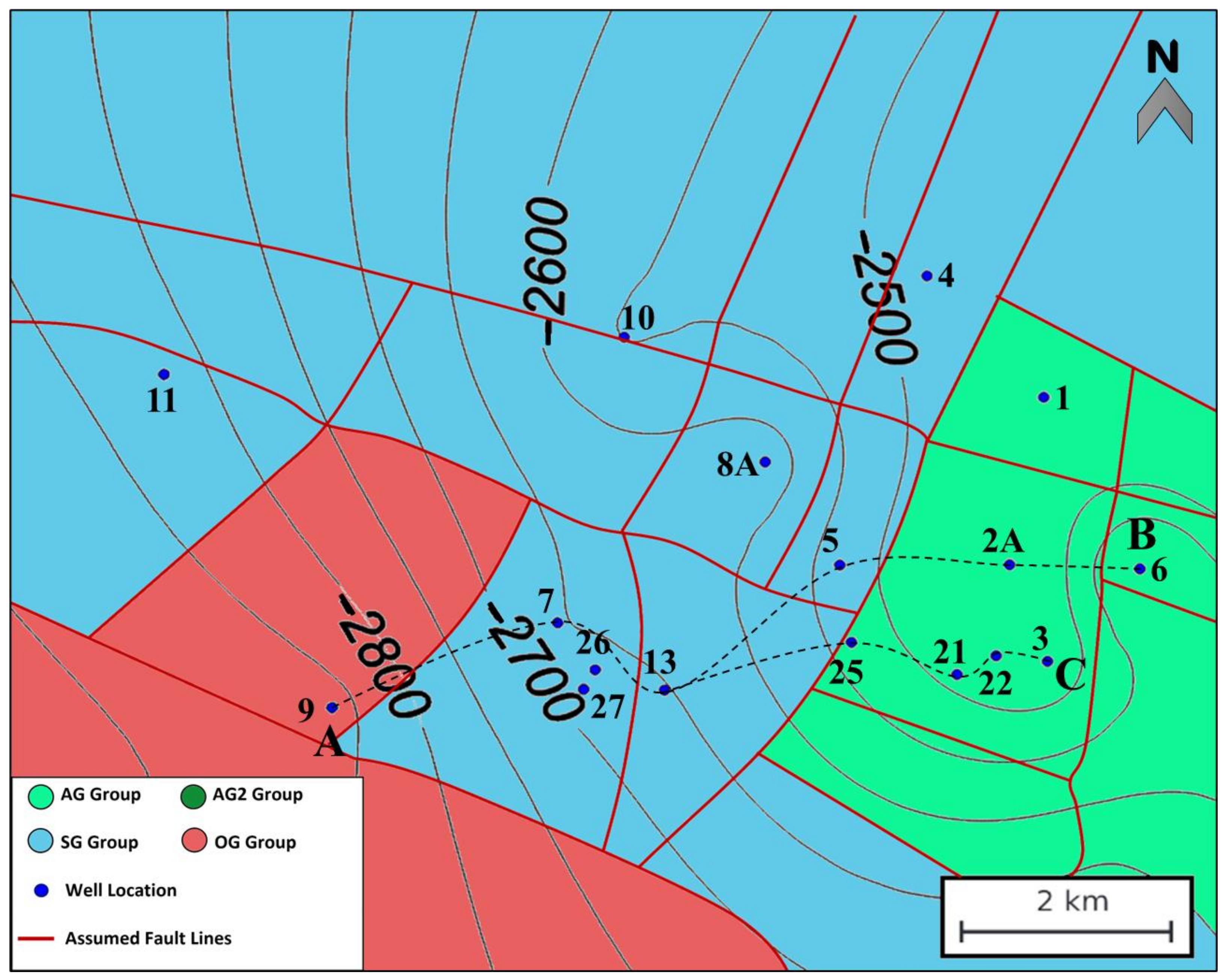
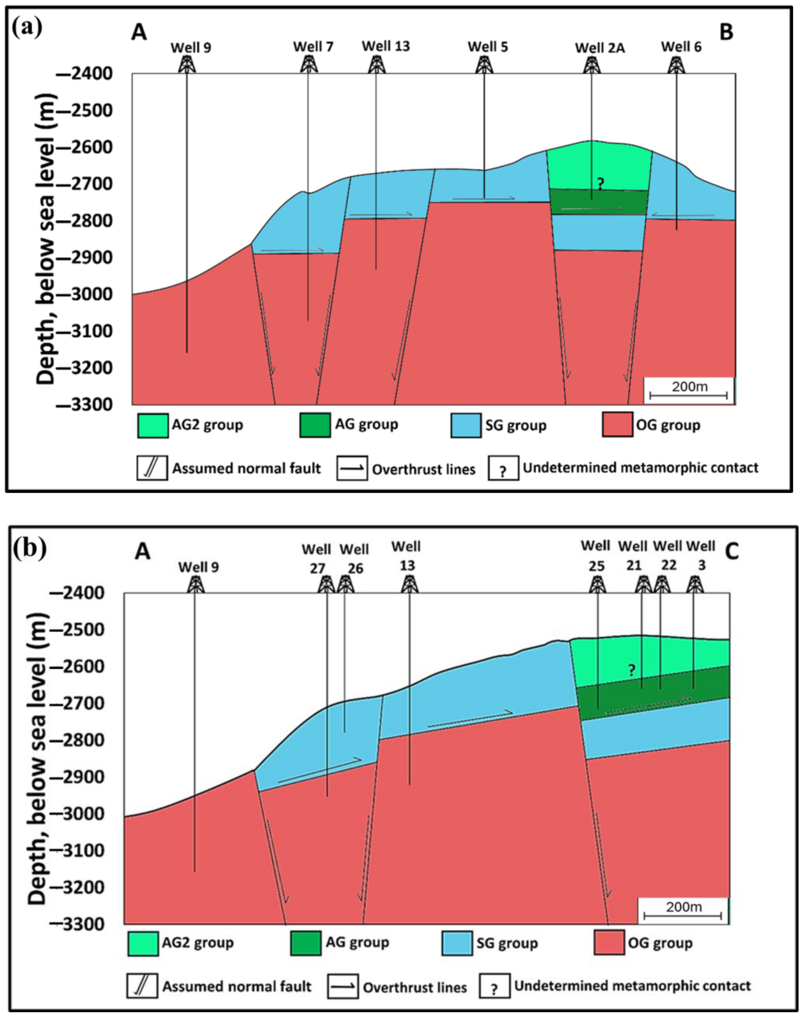
2. Geological Setting

The Pannonian Basin of Hungary has undergone several geological events that resulted in a very complex mosaic of basement blocks [41,42,43]. This pre-Neogene assemblage is composed mainly of Variscan metamorphic rocks of diverse metamorphic and structural evolutions [44]. Based on the evidence of previous studies [41,42,45,46], several sections of the basement act as a buried hill fractured fluid reservoir, which not only acts as a conduit, but also stores a significant amount of hydrocarbon. The studied area is Mezősas field, where numerous wells have penetrated the fractured crystalline basement and produced hydrocarbon [47,48].

During the Cretaceous, complex nappe systems were formed throughout the metamorphic realm due to Eoalpine compressional tectonic evolution [41,49]. The basin formation during the Neogene resulted in the subsidence of deep sub-basins and the exhumation of crystalline highs among them. Due to such subsequent tectonic activities, blocks of significantly different metamorphic evolutions were juxtaposed and built up the basement highs. These blocks are usually separated by structural features such as normal and overthrust faults [44,45]. Due to the ongoing subsidence, these highs became buried 1–5 km beneath the present surface. These buried hills have been the leading interest for decades since they are highly fractured and active for hydrocarbon exploration and production [46,47,50].

The Mezősas high and the surrounding basement high (Szeghalom, Furta, etc.) areas have been studied extensively regarding petrology, structural evolution, and fracture tendencies [43,44,45,46,51]. Three major rock bodies build the basement [52,53]. Orthogneiss (OG block) dominates the lowermost zone, followed by garnet- and sillimanite-bearing paragneiss (SG block). Finally, amphibolite and amphibole biotite gneiss (AG block) occur on the topmost section. Figure 1 shows the simplified geological map of the study area with the location of several wells that penetrated the basement.

The topmost AG block is the reservoir’s most highly fractured rock body and is responsible for the most significant hydrocarbon accumulation and storage [46,54]. Figure 2a,b show the cross-sections of the area along the lines marked in Figure 1. The figures also show the position of the most essential, large-scale structures that define block boundaries inside the basement. Previous studies proved that these structures are responsible for the fluid migration inside the reservoir [44,47]. The existence of these structures explains the accumulation of hydrocarbon in the fractured AG body.

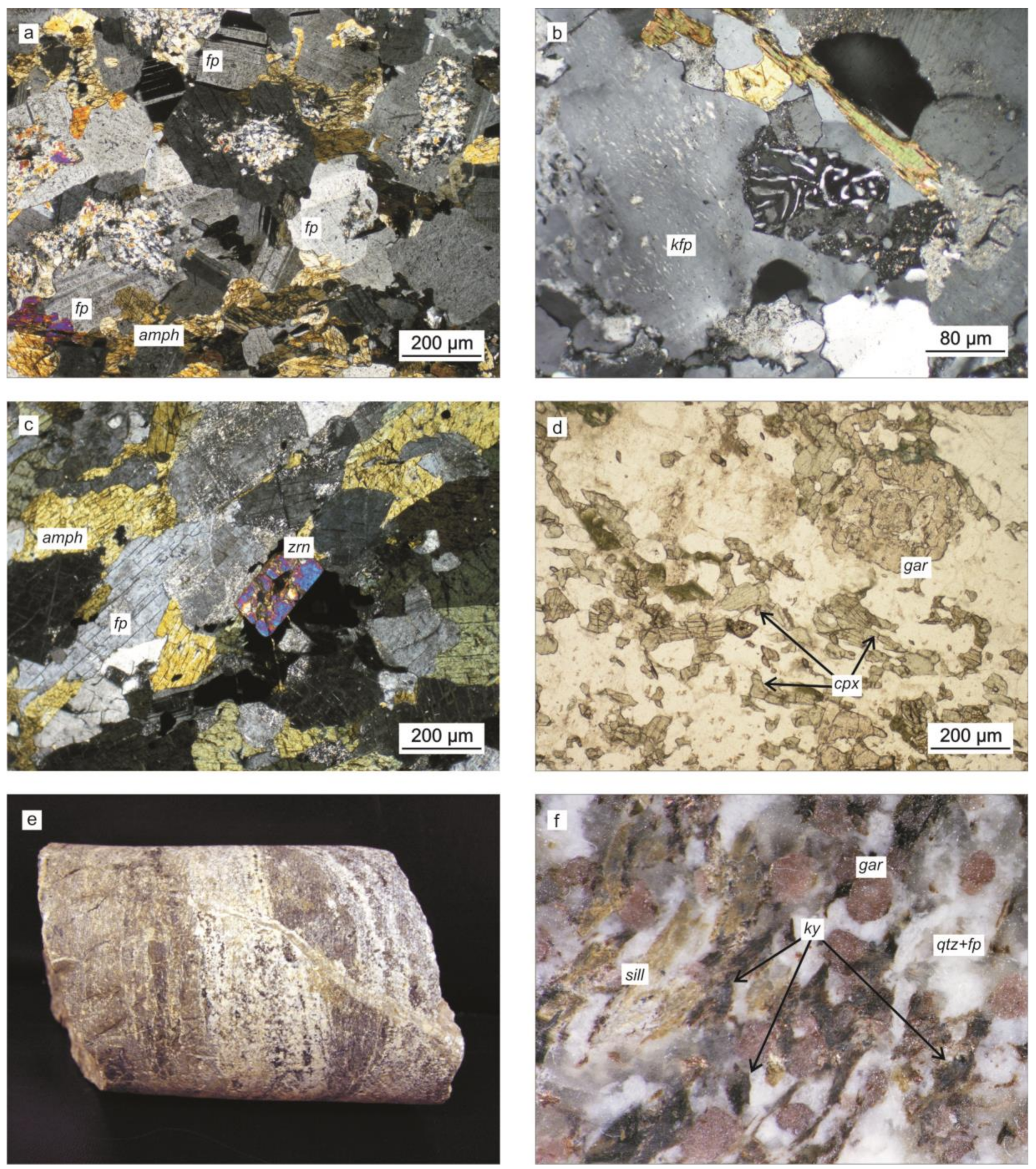
Petrography of the Rock Bodies

Both rock bodies compared in this study consist of quartz–feldspar gneisses. The lowermost structural unit shows unequivocal characteristics of orthogneisses, like relic polygonal quartz–feldspar microtextures (Figure 3a), myrmecitic feldspar grains (Figure 3b), and idiomorphic accessories (Figure 3c). As the most frequent rock-forming phases are quartz and feldspar, and the amount of micas is low, the rock has a gneissic structure. The most special petrographic feature of the rock type is that it usually contains garnet, clinopyroxene, and amphibole xenocrysts (Figure 3d). Occasionally, xenoliths of a relatively broad spectrum of rock types also occur. So far, diverse amphibolite varieties, eclogite, felsic granulite, and forsterite marble have been described and evaluated petrologically (Figure 3e,f). Refs. [52,54] found that the xenoliths preserve significantly different metamorphic evolutions, but all were recrystallised afterwards under the physical conditions where the orthogneiss formed. Based on the current interpretations [54], the original granitoid protolith of the orthogneiss realm intruded an accretionary prism, where it could pick up the xenoliths. Such evolution led to the development of the unique and, at large scale, heterogeneous internal structure of the OG body.

In contrast, the overlying block is interpreted as paragneiss. It lacks all of the above textural and structural features; the accessories are xenomorphic in shape, but these samples contain significantly more mica than the typical orthogneiss. As a consequence, this rock type is more foliated. Moreover, it exhibits a polymetamorphic texture with early metamorphic garnet1 + kyanite followed by late garnet2 + sillimanite (Figure 4a,b). As the most characteristic distinctive feature of the paragneiss samples is the common presence of sillimanite bundles, this block is called sillimanite gneiss (SG) in summary.

Previously, refs. [44,50] found that the two bodies are systematically separated by a brittle tectonic zone dominated by cataclasite and fault breccia. Later, ref. [53] proved that the two gneiss varieties can be clearly distinguished using geophysical well-log data, suggesting that the above-written mineralogical and structural differences also cause reliable differences in the physical conditions of the two gneiss varieties. From a reservoir geological point of view, the critical question is whether or not the two gneiss varieties, which are slightly different in mineralogy and structure, are also different in terms of fracture density.

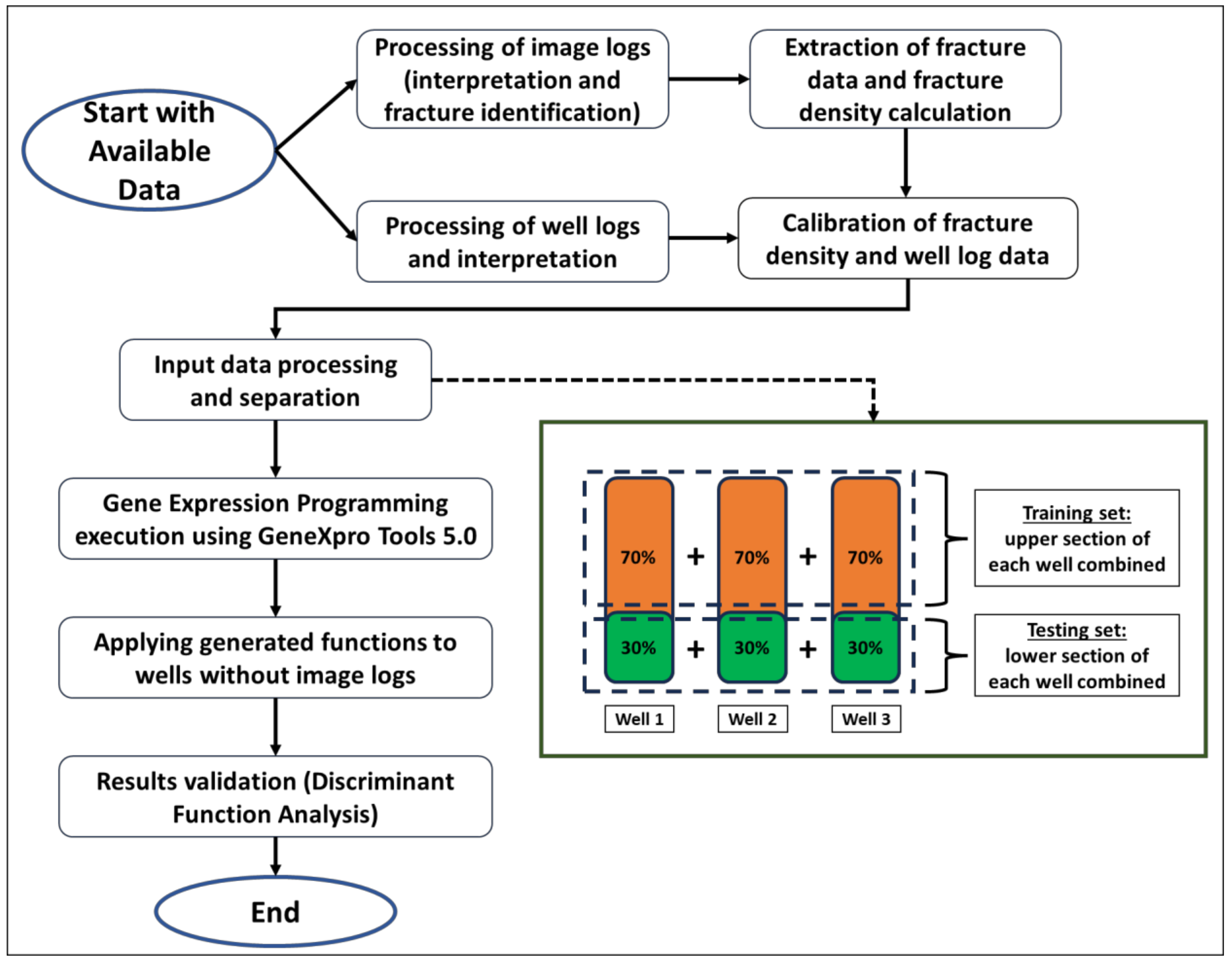
3. Samples and Methods

This study selected two different metamorphic lithologies that made up the basement reservoir of the Mezősas field, namely, SG and OG. Conventional well-logs are available for analysis: GR, K, TH, U, RD, RS, RXO, D, N, and S. In addition, image logs are also available for some wells. For SG, three wells with image logs were available and used as training datasets: Wells 7, 10, and 13. In the case of OG, Wells 7, 13, and 27 were used as training datasets. The descriptive statistics of all wells are shown in

Table 1. Descriptive statistics of Wells 7, 10, and 13, including the combination n of all three wells.

Well (Unit)		GR (API)	K (%)	Th (ppm)	U (ppm)	RD (ohm·m)	RS (ohm·m)	RXO (ohm·m)	D (g/cc)	N (v/v)	S (us/f)
7 (n = 92)	Min	60.97	2.19	3.08	1.98	0.06	0.06	0.07	2.49	4.17	57.83
(2746 m	Max	122.12	4.16	10.69	4.20	0.14	0.18	0.42	2.69	15.41	65.88
–	Mean	78.47	2.80	5.49	2.70	0.10	0.12	0.20	2.63	10.55	61.33
2896.5 m)	SD	14.50	0.41	1.79	0.64	0.02	0.03	0.09	0.05	2.40	1.94
10 (n = 114)	Min	83.90	1.85	5.79	2.33	0.10	0.08	0.10	2.59	10.00	60.31
(2641 m	Max	176.61	3.46	15.24	5.33	0.18	0.23	0.21	2.81	19.00	68.03
–	Mean	115.09	2.74	9.53	3.52	0.14	0.16	0.16	2.68	14.09	63.34
2813 m)	SD	19.93	0.45	1.99	0.76	0.02	0.04	0.03	0.06	2.47	2.15
13 (n = 96)	Min	63.29	1.29	2.23	4.29	0.12	0.18	0.12	2.63	3.49	58.60
(2690 m	Max	153.39	3.95	11.38	5.59	0.30	0.44	0.33	2.89	15.48	74.44
-	Mean	104.78	2.52	5.98	4.97	0.20	0.31	0.21	2.73	10.65	66.09
2769.8 m)	SD	29.42	1.01	2.60	0.34	0.06	0.08	0.07	0.08	3.70	5.27
All wells (7, 10, 13)	Min	60.97	1.29	2.23	1.98	0.06	0.06	0.07	2.49	3.49	57.83
	Max	176.61	4.16	15.24	5.59	0.30	0.44	0.42	2.89	19.00	74.44
	Mean	97.81	2.68	7.14	3.45	0.14	0.17	0.18	2.67	12.00	62.86
	SD	28.00	0.58	2.98	1.06	0.05	0.08	0.07	0.07	3.29	3.62

Abbreviations: gamma ray (GR), potassium (K), thorium (TH), uranium (U), deep resistivity (RD), flushed zone resistivity (RXO), bulk density (D), neutron porosity (N), sonic porosity (S), and photoelectric effect (PE). Min: minimum value; Max: maximum value; SD: standard deviation.

and

Table 2. Descriptive statistics of Wells 7, 13, and 27, including the combination n of all three wells.

Well (Unit)		GR (API)	K (%)	Th (ppm)	U (ppm)	RD (ohm·m)	RS (ohm·m)	RXO (ohm·m)	D (g/cc)	N (v/v)	S (us/f)
7 (n = 78)	Min	45.56	2.02	2.29	1.06	0.04	0.05	0.07	2.57	6.79	54.00
(2896.5 m	Max	63.22	2.75	3.47	1.90	0.13	0.16	0.55	2.67	13.45	60.35
–	Mean	55.30	2.40	3.10	1.48	0.10	0.12	0.26	2.63	10.29	57.55
3080 m)	SD	4.84	0.23	0.34	0.17	0.03	0.03	0.13	0.03	1.53	1.83
13 (n = 122)	Min	89.42	2.05	2.48	4.65	0.03	0.07	0.03	2.63	1.71	53.36
(2769.8 m	Max	175.25	3.95	16.64	6.30	0.14	0.34	0.18	2.86	9.97	65.14
–	Mean	116.66	2.73	6.77	5.38	0.07	0.14	0.08	2.72	4.59	57.20
2955 m)	SD	17.74	0.43	3.18	0.46	0.03	0.06	0.04	0.06	2.62	2.77
27 (n = 46)	Min	75.01	2.35	4.22	1.26	0.03	0.04	0.04	2.64	7.25	56.47
(2885 m	Max	85.66	3.13	6.18	4.27	0.08	0.10	0.12	2.69	10.85	59.59
-	Mean	80.07	2.77	5.16	2.13	0.06	0.07	0.08	2.66	8.44	57.96
2945 m)	SD	3.62	0.23	0.70	0.95	0.01	0.02	0.03	0.02	1.16	0.86
All wells (7, 13, 27)	Min	45.56	2.02	2.29	1.06	0.03	0.04	0.03	2.57	1.71	53.36
	Max	156.13	3.51	14.44	6.30	0.14	0.34	0.55	2.86	13.45	65.14
	Mean	88.23	2.57	4.99	3.55	0.08	0.12	0.14	2.68	7.10	57.29
	SD	29.07	0.33	2.15	1.96	0.03	0.05	0.13	0.06	3.36	2.38

Abbreviations: gamma ray (GR), potassium (K), thorium (TH), uranium (U), deep resistivity (RD), flushed zone resistivity (RXO), bulk density (D), neutron porosity (N), sonic porosity (S), and photoelectric effect (PE). Min: minimum value; Max: maximum value; SD: standard deviation.

for SG and OG, respectively. The data show each of the well-log parameters’ minimum, maximum, mean, and standard deviation values of each training well, including the data of all wells combined.

The analysis started with image log processing. The type of image log used in this study is the Circumferential Borehole Image Log (CBIL). As mentioned, the available raw data from image logs for certain wells were interpreted, and fracture zones were determined. CBIL scans the borehole in a rotational manner and, as a result, the cylinder images are produced as raw data. These raw data are then displayed in rectangular form using image processing software. The images are presented in static and dynamic normalized form in which the latter normally shows the enhanced contrast for recognizing the fractures more easily [55]. These static and dynamic images are shown after corrections such as speed correction, eccentering correction, normalization, and image filtering have been conducted [56,57,58]. The image logs recorded the sonic travel time and amplitude [59]. The dark sinusoidal wave displayed on the image logs normally indicate fractures with low acoustic amplitudes [60]. Each fracture was handpicked, and the fracture type was determined. The fractures were classified into open, closed, partially open, and induced fractures. On the dynamic normalized image log, the open fractures are shown by both the amplitude and travel-time images while closed fractures are indicated by the amplitude image [61]. Once the fractures had been identified, the FD was calculated. In general, FD is the number of fractures per unit length, and in this study, the number of fractures per metre was used. Therefore, the unit is m⁻¹. By definition, fracture density can also be defined as cumulative fracture trace length per unit area (sometimes referred to as areal intensity) or cumulative fracture area per unit volume [12].

The well-log data were then integrated with the FD data calculated earlier. The quality of the well-log data was checked thoroughly so that bad data such as missing points were assessed, and extreme outliers were removed. Since the FD data were calculated per metre length, the well-log data were also calculated per metre length. The descriptive statistics shown in Table 1 and Table 2 are based on these resampled data. After that, the data from all three training wells for SG and three wells for the OG rock column were divided into two sets: the training set and the testing set. The workflow of this study is shown in Figure 5.

The training set consisted of 70% of the data (taken from the upper section of the well), and the testing set consisted of 30% (taken from the lower section). The illustration of this concept is also shown in Figure 5. The training set from all SG rock column wells was combined and was run for the GEP modelling using GeneXpro Tools 5.0. The same process was applied to the OG rock column dataset as well.

Before running the GEP simulation, a correlation study was conducted between input variables (well-log parameters) and output variables (FD values) to see whether or not any well-log parameters highly correlate to FD. The correlation results are shown in Figure 6 for all wells used for SG training data and Figure 7 for all wells used for OG training data. Individual well correlation studies were also conducted, but generally, the results for each correlation study were the same throughout all wells. Hence, in this paper, we combined all data from all wells to show that none of the well-log parameters were highly correlated to FD. Therefore, all of these well-log parameters were selected for input parameters for GEP. As GEP is a robust method, it means that the prediction or input variables for GEP are not required to be normally distributed. GEP works by identifying the best functions by generating and iterating chromosomes when necessary.

GEP is an advanced machine learning method that mimics human genetics [62]. As the genes in the human chromosome contain heads and tails, so does the chromosome structure in GEP. The chromosome structure is produced vigorously, as shown in Figure 8. The process starts with the creation of the initial population’s chromosome, and these chromosomes are expressed in the expression tree (ET) [63,64]. The mathematical equation can be written from the ET [65,66]. Each chromosome is executed, and the fitness is evaluated. If the best solutions are met, then the process will be stopped. However, if it is not, the chromosome will be reiterated by numerous processes such as mutation, replication, transposition, and recombination to create new ETs [39,67]. The same evaluation process is repeated until the best solutions or predefined fitness are achieved [68,69,70].

Figure 9a shows an example of chromosome structure in ET. Chromosomes can be made up of one or more genes. The gene contains a head and a tail, as shown in Figure 9b. The head in GEP can contain both function and terminal, while the tail contains only the terminal [39,71]. For example, in Figure 9, a mathematical expression is written as the $\sqrt{\left(x_1+c\right)}+\ln \left(x_2-x_3\right)$; the expression is written based on the ET and Karva language developed by [39].

Once the results and equations had been generated by GeneXpro Tools 5.0, the equations were applied to the other remaining wells without image logs or FD data. To evaluate the performance of the models developed by GEP, RMSE and MAE were calculated as proposed by previous studies [72,73,74,75,76,77,78]. The equations for calculating RMSE and MAE are shown in Equations (1) and (2), respectively.

$$RMSE=\sqrt{\frac{{\Sigma }_{i=1}^n{\left(e_i-m_i\right)}^2}{n}}$$

(1)

$$MAE=\frac{{\Sigma }_{i=1}^n\left|e_i-m_i\right|}{n}$$

(2)

where n is the overall data points, m_i is the model outcome value, and e_i is the experimental value. Low RMSE and MAE show a well-calibrated model. Additionally, the results from GEP modelling produced functions consisting of well-log parameters. From this result, a sensitivity analysis (SA) was performed to investigate the relative contribution of the well-log variables generated by the GEP model. In this case, SA was calculated using Equations (3) and (4), as proposed in the literature [79,80,81,82].

$$N_i=f_{max}\left(x_i\right)-f_{min}\left(x_i\right)$$

(3)

$$SA=\frac{N_i}{{\sum }_n^{j=1}{N}_j}$$

(4)

where x_i is the ith input variable, f_max(x_i) is the maximum value of outcome, and f_min(x_i) is the minimum value of the outcome that depends on its ith input dominion, in which other input variables are maintained at a constant average value. The difference between f_max(x_i) and f_min(x_i) gives the range N_i of the ith input variable.

Then, the results were validated using the discriminant function analysis (DFA) method. DFA is a multivariate statistical approach used to predict group memberships based on prior knowledge of existing group memberships [83]. In DFA, there are independent variables and dependent variables. The aim is to predict group memberships or dependent variables based on the input from independent variables [84,85]. In this case, the results from GEP were used as inputs for the DFA that was run using IBM SPSS Statistics 24 software. A more detailed flow process of this method is shown in Figure 10. Finally, a well-to-well correlation model was proposed based on the overall FD values from other wells.

4. Results

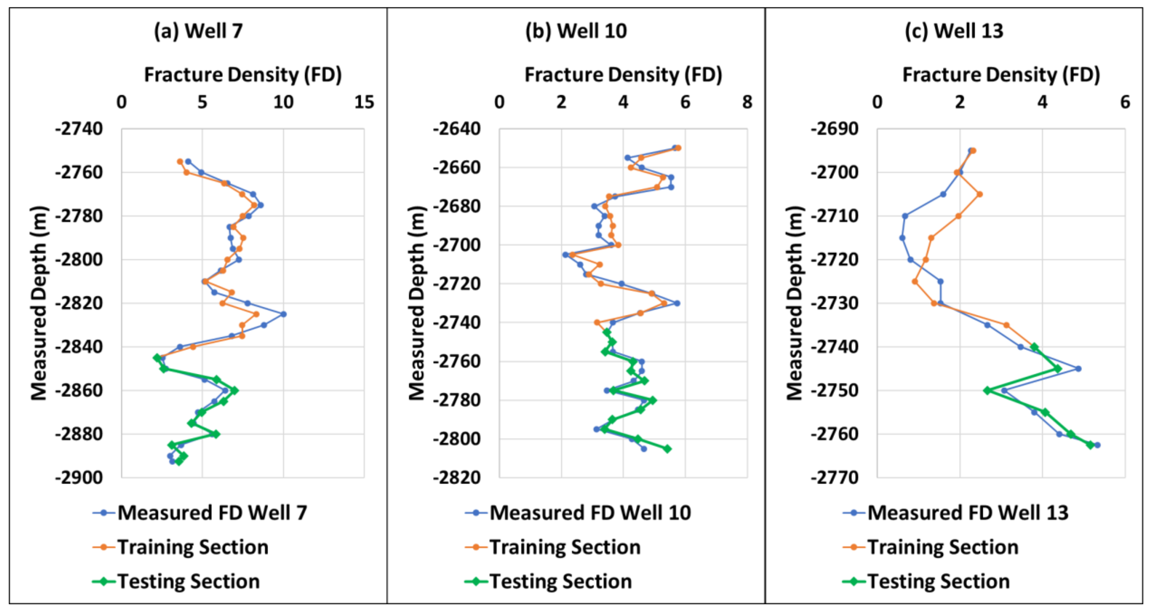
4.1. Training and Testing for SG Rock Column

As mentioned earlier, for the SG rock column, Wells 7, 10, and 13 with measured FD data from the image logs were used as the training and testing sets in the GEP. The results from the GEP process are shown in Figure 11. The blue lines are the measured FD from the image logs, the orange line is the section taken for the training set, and the green line is the dataset used as the testing set. The results show that the predicted FD values for the lower section of the well were consistent with the measured FD values.

To evaluate the results produced by GEP, the coefficient of determination (R²) was used to determine whether the results were acceptable. The measured and predicted FD values were plotted, and R² values were calculated, as shown in Figure 12. All three wells showed good R² values. For instance, Well 7 showed an R² value of 0.86, Well 10 showed a value of 0.86, and Well 13 showed a value of 0.88. After GEP produced the results, Equation (5) was generated. The equation was produced based on the expression tree shown in Figure 13. Finally, four sub-ETs were produced based on the GEP modelling. Each of these sub-ETs makes up Equation (5). The equations for each sub-ET are shown in Equations (6) to (9), in which Equation (6) is for sub-ET 1, Equation (7) is for sub-ET 2, and so on.

$$F{D}_{SG}=S{G}_1+S{G}_2+S{G}_3+S{G}_4$$

(5)

$$S{G}_1=\frac{\left[\frac{1}{\left(D^{\ast }TH\right)-Exp\left(U\right)}\right]+\left[{\left(D+\left(-1.85\right)\right)}^2+(\frac{\left(K+\left(-0.71\right)\right)}{2}+U)\right]}{2}$$

(6)

$$S{G}_2={\left(\left[\left(\frac{1}{RD}+\left(K+TH\right)\right)+\left(\left(D-9.39\right)-\left(RX0-\left(-9.10\right)\right)\right)\right]-RXO\right)}^{\raisebox{1ex}{$1$}\!\left/ \!\raisebox{-1ex}{$3$}\right.}$$

(7)

$$S{G}_3={\left(K\right)}^{1∕3}\ast \mathrm{Atan}\left[{\left(TH-\frac{K}{RD}\right)}^{\ast }\left(\frac{\min \left(7.91,TH\right)+(-7.12)}{2}\right)\right]$$

(8)

$$S{G}_4=\mathrm{Atan}\left[\left(\frac{{\left(\frac{-8.58+1.72}{2}\right)}^{\raisebox{1ex}{$1$}\!\left/ \!\raisebox{-1ex}{$3$}\right.}+\left(\frac{\left(TH-U\right)+K}{2}\right)}{2}\right)\ast \left(Exp\left(U\right)\ast \left(\frac{RXO+D}{2}\right)\right)\right]$$

(9)

Equation (5) was then applied to the other wells with no image logs to predict the FD values. The equation was applied to the SG rock column of Wells 4, 6, 8, 11, and 26. The results of this process are shown in Figure 14. Although it cannot be confirmed at this point that the predicted FD values are accurate, based on the results shown in Figure 14, the range of FD values is consistent between wells and comparable to the training wells. Notice that from Equations (6) to (9), although ten well-log parameters were entered as inputs, only six parameters appeared in these equations. GR, RS, N, and S did not appear in these equations.

4.2. Training and Testing for OG Rock Column

The same process for the SG rock column was applied to the OG rock column data. Three wells with image logs and fracture density data were processed in the GEP tool. As shown in Figure 15, the training section dataset was taken from the upper part of each well and combined. As for the testing section, the lower part of the dataset for each well was used, and the testing section results aligned with the measured fracture density data.

The R² values for each well were calculated by plotting the predicted FD values against the measured FD values. The results are shown in Figure 16, in which for Well 7, the R² value is 0.85, for Well 13 is 0.86, and for Well 27 is 0.90. These results show that the model prediction can be accepted.

The expression tree results produced by GEP modelling are shown in Figure 17. Based on this expression tree, Equation (10) was derived. The equation was then applied to the other five wells without image logs and FD data: Wells 4, 8, 9, 10, and 11. As in the results for OG, there were four sub-ETs, and Equation (10) was a combination of Equations (11) to (14), which were written based on the four sub-ETs in Figure 17. Equation (11) was written based on sub-ET 1, Equation (12) was based on sub-ET 2, and so on. Figure 18 shows the results of the FD calculation using Equation (6) for Wells 4, 8, 9, 10, and 11.

$$F{D}_{OG}=O{G}_1+O{G}_2+O{G}_3+O{G}_4$$

(10)

$$O{G}_1=\frac{U+{\left[{\left(RD-\frac{1}{0.89}\right)}^{\ast }\left({\left(U-TH\right)}^{\ast }\left(R{D}^{\ast }N\right)\right)\right]}^2}{2}$$

(11)

$$O{G}_2=\mathrm{Atan}\left[{\left(\max \left(U,TH\right)+\left(-4.98+RXO\right)\right)}^{\ast }\left(\max \left(N^2,3.25\right)\right)-\ln \left(\frac{1}{RXO}\right)\right]$$

(12)

$$O{G}_3=\min \left(1-\left(\ln \left(U\ast U\right)\ast \left(R{D}^{\ast }K\right)\right)\ast 3.32,{\left(U\right)}^2\right)$$

(13)

$$O{G}_4=\frac{1}{\left[\max \left(\left(8.49+TH\right),\left(K+N\right)\right)-\left(\left(-4.95\right)\ast \left(-2.99\right)\right)\right]-\left[\frac{\left((-2.95\right)\ast TH)+(9.90-U)}{2}\right]}$$

(14)

From Equations (11) to (14), it can be seen that not all ten parameters appeared in all equations. Only six parameters appeared in these equations from the original ten well-log parameters. GR, RS, D, and S parameters did not appear in any of them.

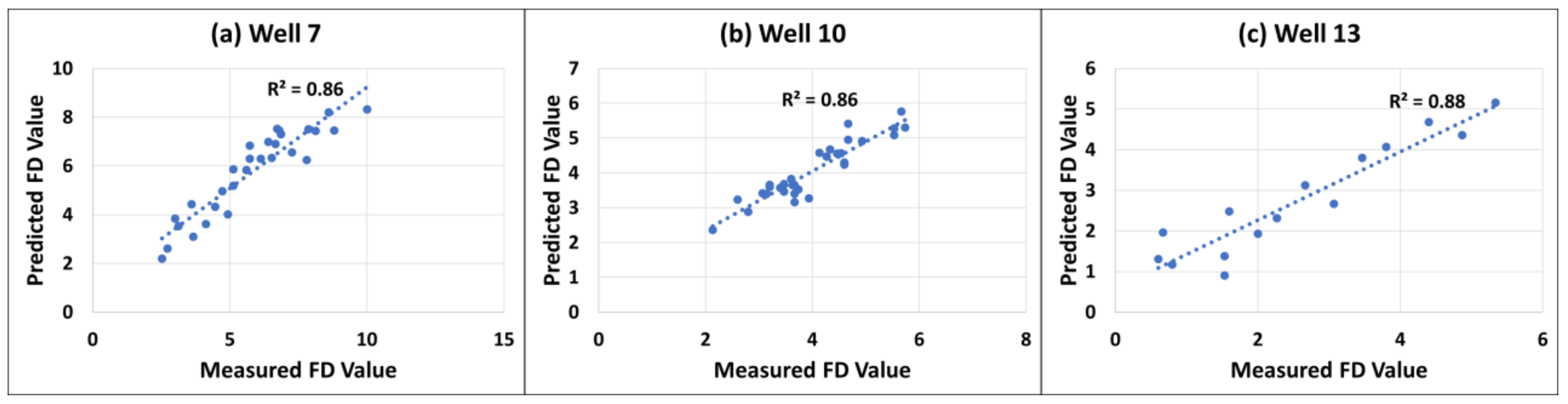
4.3. Performance Evaluation of GEP Models

GEP models can be evaluated statistically using RMSE and MAE results. Other than these two parameters, R² is a good performance indicator as well, which was described in the previous section. A well-calibrated model will have low RMSE and MAE values. Based on these criteria, the calculated values of RMSE and MAE are shown in

Table 3. Statistical results for evaluating the GEP model’s performance.

	SG		OG
	Training	Testing	Training	Testing
RMSE	0.63	0.4	0.55	0.42
MAE	0.49	0.34	0.38	0.30

. The results for SG and OG are shown, and the training and testing results are shown separately. It is indeed proven that the developed model based on GEP simulation works well based on the RMSE and MAE values in Table 3. For the SG rock body, for instance, the RMSE and MAE values are low for the training dataset and the values are even lower for the testing dataset. The same trend is seen for the OG results, in which both RMSE and MAE values are low for the training dataset and even lower for the testing dataset. This shows that the GEP model is well calibrated statistically.

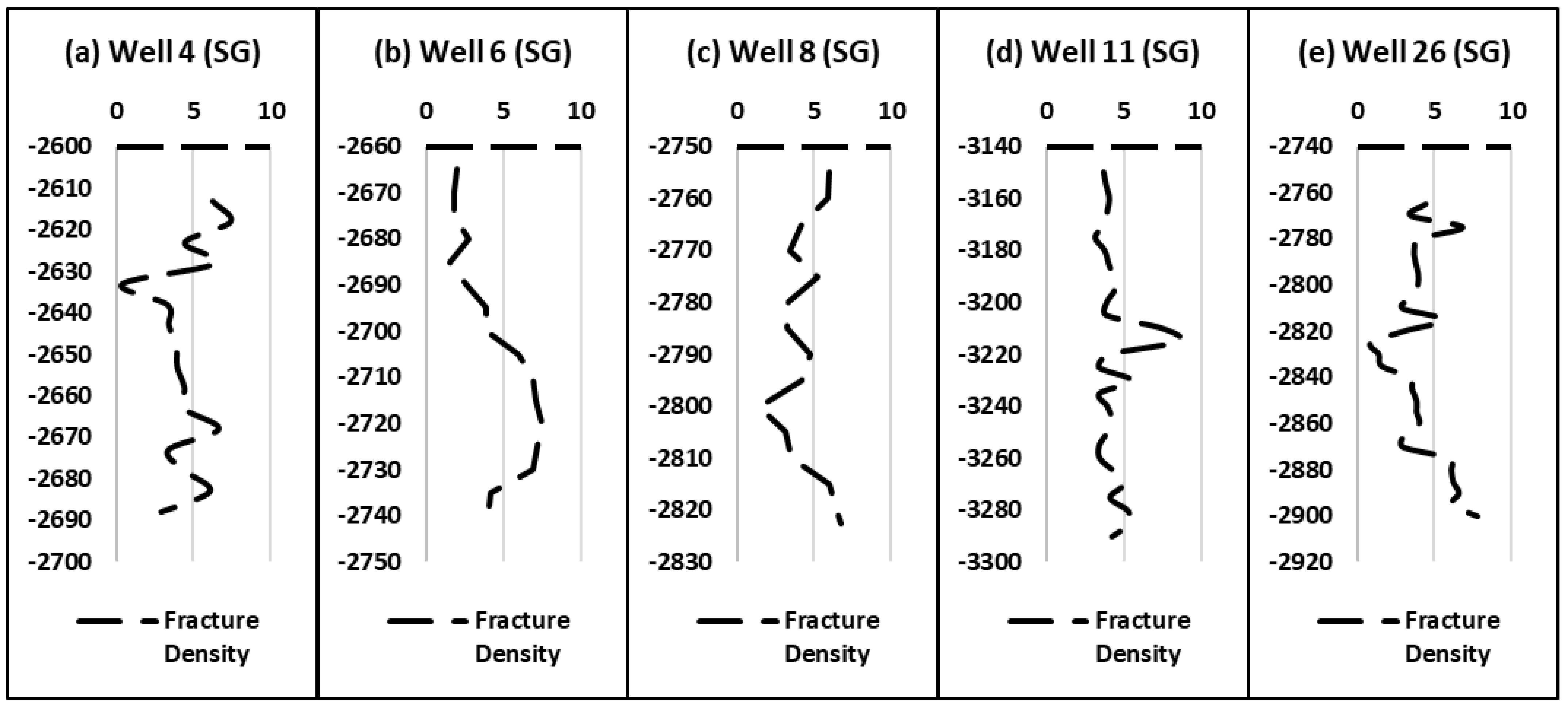
4.4. Validation of Fracture Density Predictions

It is challenging to validate the predicted FD values of wells without image logs and core samples. However, this can be achieved by comparing the well-log properties and the trends of the wells with image logs with those of the wells without the image logs using statistical analysis. In this case, DFA was chosen. As can be seen from Equations (5) to (9) for SG FD predictions, six well-log properties appeared in the equations out of the ten initial well-log properties used as inputs for GEP modelling. The properties are K, TH, U, RD, RXO, and D. Similarly, for OG FD predictions, six well-log properties appeared in Equations (10) to (14): K, TH, U, RD, RXO, and N. These well-log properties were used as predictor variables or independent variables in the DFA, as shown in Figure 10. The FD values were grouped into the low FD and high FD groups, which were the dependent variables in the DFA. This grouping is illustrated in Figure 19a. In Figure 19a, the data selected for the low FD zone are highlighted in red, and the high FD zone is highlighted in blue. The red and blue highlights were placed on the black dashed line that shows the FD values. Using this method, the primary assumption is that the low and high FD values were correctly measured and determined, while the middle FD values were not grouped, as these middle values were considered grey areas. This means that the FD values in the middle neither belong to low nor high FD values. If a cutoff line were to be drawn to separate the low and high FD values, there is no concrete way to do this accurately. A simple average method could be adopted; however, it may underestimate or overestimate the separation.

The results for the SG group are shown in Figure 19 and Figure 20. Figure 19 shows the results of the DFA applied to Well 10. Figure 19a shows the measured FD values in a black dashed line with the highlighted dataset selected for low and high FD values. After running the DFA using the inputs shown in Figure 18 for the SG group, the results were obtained and are shown in Figure 19b, which shows the eigenvalue, canonical correlation, and histogram plot of the discriminant score. The function generated from the DFA was then applied to the whole dataset of Well 10; the discriminant score results are plotted in Figure 19a and are shown as a blue line. Comparing the FD and discriminant score plots in Figure 19a, both plots are in agreement with one another and have similar trends. These results show that the inputs chosen to predict FD values from the earlier GEP modelling can be accepted. However, at specific depths on the plot, the discriminant scores suggest lower or higher trends than the FD values. Hence, the validation method shown here is suitable for validating and checking the consistency of the predicted FD values through GEP modelling. Therefore, the same DFA method was applied to the wells without an image log to ensure that the predicted FD values from the GEP modelling can be validated. Similar trends are expected from wells without the image logs.

Figure 20 shows two wells without image logs, but the FD values were generated from GEP modelling prediction. Figure 20a shows the FD values of Well 6. For this well, it is clear that two separate FD values can be grouped into low and high FD values, showcased by a black dashed line. DFA was conducted for this well using the inputs mentioned in Figure 18, and the results of the DFA are shown in Figure 20b. The eigenvalue and canonical correlation results are in the acceptable range. Based on this result, a function was generated and applied to the Well 6 dataset; hence, a blue line was plotted, as shown in Figure 20a, which is the discriminant score. The FD values and discriminant score show similar trends, and the results agree with the result for Well 10 shown in Figure 19. This means that the FD values generated by GEP modelling can be accepted and validated in the case of Well 6. Similarly, the same process described above was applied to another well, Well 8, and the results are shown in Figure 20c,d. Although the discriminant score shown in Figure 20c at specific depths shows high values, for instance, at depths from −2765 m to −2790 m, the discriminant score still has a similar trend as the predicted FD values on the same plot, and the results are consistent with the trend of the results for Well 10 shown in Figure 19. Hence, the predicted FD values from GEP for Well 8 are also validated.

The same method was applied to the OG group. As a primary reference, the DFA method was applied to the well with image logs, and an example for this case, Well 13, was selected and is shown in Figure 21. Figure 21a shows the FD values with highlighted zones where low and high FD values were chosen for the DFA process. The results of the DFA are shown in Figure 21b, with an eigenvalue of 1.142. Based on this process, the generated function was applied to the Well 13 dataset, and a plot of the discriminant score is shown in Figure 21a as a blue line. The results show that the FD values and discriminant score have similar trends and can predict the low and high FD zones well.

The method was then applied to the wells without image logs, as shown in Figure 22. For example, Wells 4 and 10 are shown in this case. The results of Well 4 are shown in Figure 22a,b, and the results of Well 10 are shown in Figure 22c,d. The results of both wells show that the DFA method can be used to group and separate the low and high FD groups; the generated function from the DFA can also be used to confirm the grey area values and trends. Most importantly, the results of these wells without image logs have similar trends to the wells with image logs. In this case, the predicted FD values from GEP modelling are validated and can be used.

5. Discussion

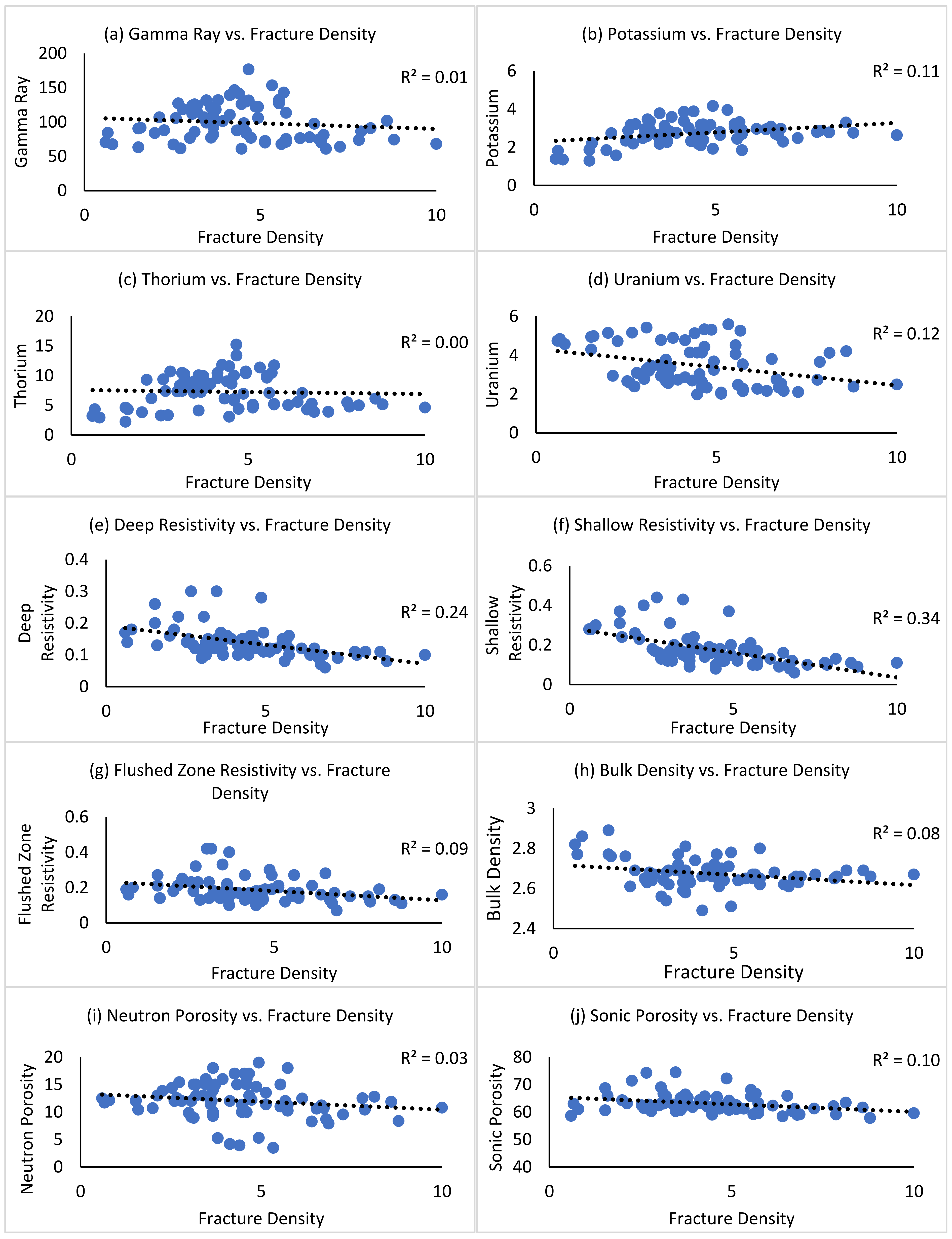
5.1. Well-Log Responses towards Fracture Characteristics

This study explored the potential of using GEP to predict FD in metamorphic rock bodies using inputs from 10 conventional well-log data. The study used wells with image logs to extract FD data and used these data as the primary training sets in GEP. The results of the GEP modelling can be used for wells without image logs; subsequently, the FD data of those wells can be predicted. Using this method, two different rock types in a produced buried hill hydrocarbon reservoir were assessed to evaluate any differences between the fracture characteristics of the two metamorphic rocks: SG and OG.

Based on the above results, there is not much difference between the SG and OG fracture density from the well-log perspective. For SG, the results from GEP modelling show that the significant well-log parameters that might have contributed to the prediction of FD based on Equation (5) are potassium, thorium, uranium, deep resistivity, flushed zone resistivity, and bulk density. In contrast, for OG, the parameters processed by GEP modelling that contributed to FD predictions based on Equation (10) were potassium, thorium, uranium, deep resistivity, flushed zone resistivity, and neutron porosity. These results show that spectral gamma ray, resistivity, and porosity are significant for FD prediction, as reported in the literature. Furthermore, there is no significant difference between SG and OG fracture properties. However, sensitivity analysis was conducted to evaluate the relative contribution of each well-log parameter to the FD prediction. These analysis results for SG and OG are shown in Figure 23a and Figure 23b, respectively. Although the six parameters narrowed down from GEP are not much different between the two rocks, based on this SA, the contribution of each well-log parameter differs.

For instance, for SG, the main three parameters based on this SA result are Th, RD, and K, while the main three parameters for OG are Th, RXO, and N. Th happens to be the highest contributing well-log parameter for both rocks. The difference between the well-log contribution of both rocks is probably due to the difference in the mineral properties of these two gneisses that might affect the responses in the well-logs. Also, as well-logs mainly measure the physical properties of the rocks and fractures being filled, there might be some differences between the log responses on this matter.

As expected, based on the reported studies, the gamma ray log did not appear in both SG and OG GEP models. GR is handy for lithology identification and can contribute to determining fracture properties, but the spectral gamma ray log is superior [19]. Uranium content, for instance, can indicate a fracture zone quite well, as uranium is soluble in water and hydrocarbon [20]. Uranium concentration appeared in both equations for SG and OG. Although uranium is not a significant chemical component that makes up SG and OG, its presence in these metamorphic rocks can point to the precipitation of uranium-bearing minerals in the veins, or it could also be present in the fluids that fills the open fractures.

Due to its resolution and the nature of the operation that uses a transmitter and receiver, resistivity is one of the more valuable tools used to detect fracture zones, especially in tight formations and low-permeability reservoirs such as crystalline rock bodies [13,16,26]. During drilling, fractured rocks surrounding the well will be filled with mud or mud filtrate, usually recorded by the resistivity logs [1,33]. Since most resistivity tools can show shallow and deep resistivity values, open fracture zones will show significantly lower shallow or flushed zone resistivity values than deep resistivity values. Although resistivity tools are mainly used for the differentiation of fluids in the formation, in the context of this study, deep and flushed zone resistivities are significant for detecting fractures, as they appear in both modelled rock bodies.

Out of the three porosity logs, only bulk density appeared in the equation for the SG group, and neutron porosity appeared in the OG group equation. The porosities may have influenced the fracture characteristics of the SG and OG rocks differently; however, evaluating porosity logs might contribute to indirect indications regarding fracture detection. For bulk density logs, fractures will lower the density values of metamorphic rocks. Depending on the type of fluids in the fracture openings, the presence of gas will lower the density readings. The hydrocarbon presence in the fracture openings will affect the reading of neutron porosity as the neutron tool reads the amount of hydrogen in the rock or, in this case, the fractures. Hence, higher neutron porosity readings can indicate that fluids exist in the fractured metamorphic rocks. To effectively evaluate the fractures, bulk density and neutron porosity logs should be used and plotted together to visualise the effects of fractures on porosity logs.

In Equations (5) and (10) from the GEP modelling, the sonic porosity parameter did not appear in either equation. However, sonic porosity contributions towards fracture determination cannot be neglected. Sonic porosity is one of the best indicators of fractures, especially when image logs are unavailable [16]. Many studies in the past have been conducted in this regard, especially on older wells, and some equations have been introduced as well [6]. The fact that the sonic log parameter did not appear in both SG and OG GEP models is probably due to the close range of sonic log readings that makes the values insignificant when there are high or low FD values. However, detecting and interpreting the cycle skipping of sonic logs manually will help in terms of fracture evaluation, since it is a valid indication of fractures. The fractures eventually lower the apparent density of rock bodies, increasing the porosity readings and sonic transit time.

Evaluating fractures from conventional well-logs alone is challenging, and the integration of data from various sources such as core samples and image logs would be the best method [86]. However, due to the limitations of data, predicting fracture properties such as FD using GEP could help. In order to ensure that the GEP model could be used for this purpose, DFA was proposed in this study. The main idea of validating the GEP modelling results by DFA was to ensure that the predicted FD values of wells without image logs were in an acceptable range, or at least comparable with those of image logs. The results from GEP modelling were used as the input parameters for the DFA. If the pattern of wells with image logs is comparable and similar to those without image logs, especially for low and high FD groups, the GEP results can be accepted and validated. Hence, this analysis shows that all wells without image logs had similar trends and patterns to wells with image logs using the inputs that had been narrowed down using the GEP results.

5.2. Theoretical Concept of the Fracture Network of the Studied Area

Figure 2 shows the structural model [53] proposed in the area under study. From the model, it was proposed that normal and thrust faults separate OG and SG realms and also allow for fluid migration. Reservoir quality and fluid flow can be influenced by faulting and fault zone deformation, as reported by [3], which has been proven previously in this area [44]. Based on the FD values calculated in this study, a well-to-well correlation was carried out for four wells, as shown in Figure 1. Wells 7, 27, 26, and 13 were close to one another, and their FD logs were plotted (Figure 24). In this plot, the black dashed lines are the overthrust zones separating SG and OG, so SG is in the upper section of the well, and OG is in the lower section. Well 26 only penetrated SG. The figure suggests that the two overlying rock bodies have a similar fracture density. If most of the fractures define an interconnected fracture system, they may help fluid migration towards the overlying sedimentary reservoir [87]. In this case, the faults, overthrust zones, and complicated fracture networks provide possible pathways for fluid migration, as suggested by [21]. They mention that the system of open fractures is usually the main pathway for fluids to move in a fractured reservoir. Furthermore, a well-developed fracture network may explain significant fluid accumulation inside the basement metamorphic rock bodies. It is best to assume that most fractures in this system are open, because open fractures act as a corridor for fluids to move. In contrast, they act as a fluid migration barrier below specific depths where most fractures are closed or occur as mineralised veins [88].

In a typical sedimentary rock where the primary porosity and permeability are good enough for the fluid to move, fracture porosity might not contribute much to the fluid movement inside the sedimentary reservoir. However, fracture porosity in crystalline rock plays a vital role in fluid movement as it provides the conduit for the fluids to move from the source rock to the reservoir rock and within the reservoir rock. A mutually interconnected fracture network of a rock body usually dominates the fluid storage capability, permeability, and the direction of the fluid flow inside the reservoir [3]. Based on [89], higher FDs coincide more at large-scale fault zones. Looking at the plot in Figure 23, Wells 13 and 27 tend to have higher FD readings near the overthrust zones that separate the two lithologies. It is assumed that at the depths far from the significant overthrust horizons (i.e., at depths of −2750 m to −2850 m for Well 7 and from −2850 m to −2950 m for Well 13), the FD values are higher due to unknown fault zones at those particular depths.

Also, the distributions of fracture densities calculated for the two rock bodies reveal that they have essentially identical fracture density (Figure 25). Both FD distributions follow a negative power law distribution with somewhat similar exponents. Petrologically speaking, different rock bodies usually react differently during deformation, which could cause fracture networks of different geometric and hydrodynamic features [90,91]. However, this study shows that although SG and OG exhibit slightly different metamorphic evolutions and mineralogy, they have similar fracture types in terms of fracture density. Ref. [17] mentioned that some fracture prediction algorithms did not work in their study because of various fracture types and geometries. However, this is not the case for this study, since, from GEP modelling, the well-log responses and FD frequencies show similar parameters.

The similar FD patterns of SG and OG conform with the geological model that the rock bodies with different metamorphic evolutions became juxtaposed during the Cretaceous nappe tectonics and became intact before the whole buried hill structure was uplifted and underwent the major brittle deformation processes that led to the formation of cracks and fractures in the rock body.

6. Conclusions

This study aimed to predict fracture density (FD) when image logs and core samples are unavailable using the nonlinear regression method of gene expression programming (GEP). The process was successfully applied to two different gneiss varieties, which exist on top of one another; sillimanite- and garnet-bearing biotite gneiss (SG) and orthogneiss (OG). Previous evidence shows that they are different in mineralogy and underwent different metamorphic evolutions. This study utilised the widely available well-log data, which are gamma ray (GR), potassium (K), thorium (TH), uranium (U), deep resistivity (RD), shallow resistivity (RS), flushed zone resistivity (RXO), bulk density (D), neutron porosity (N), and sonic porosity (S). The main conclusions are summarised below.

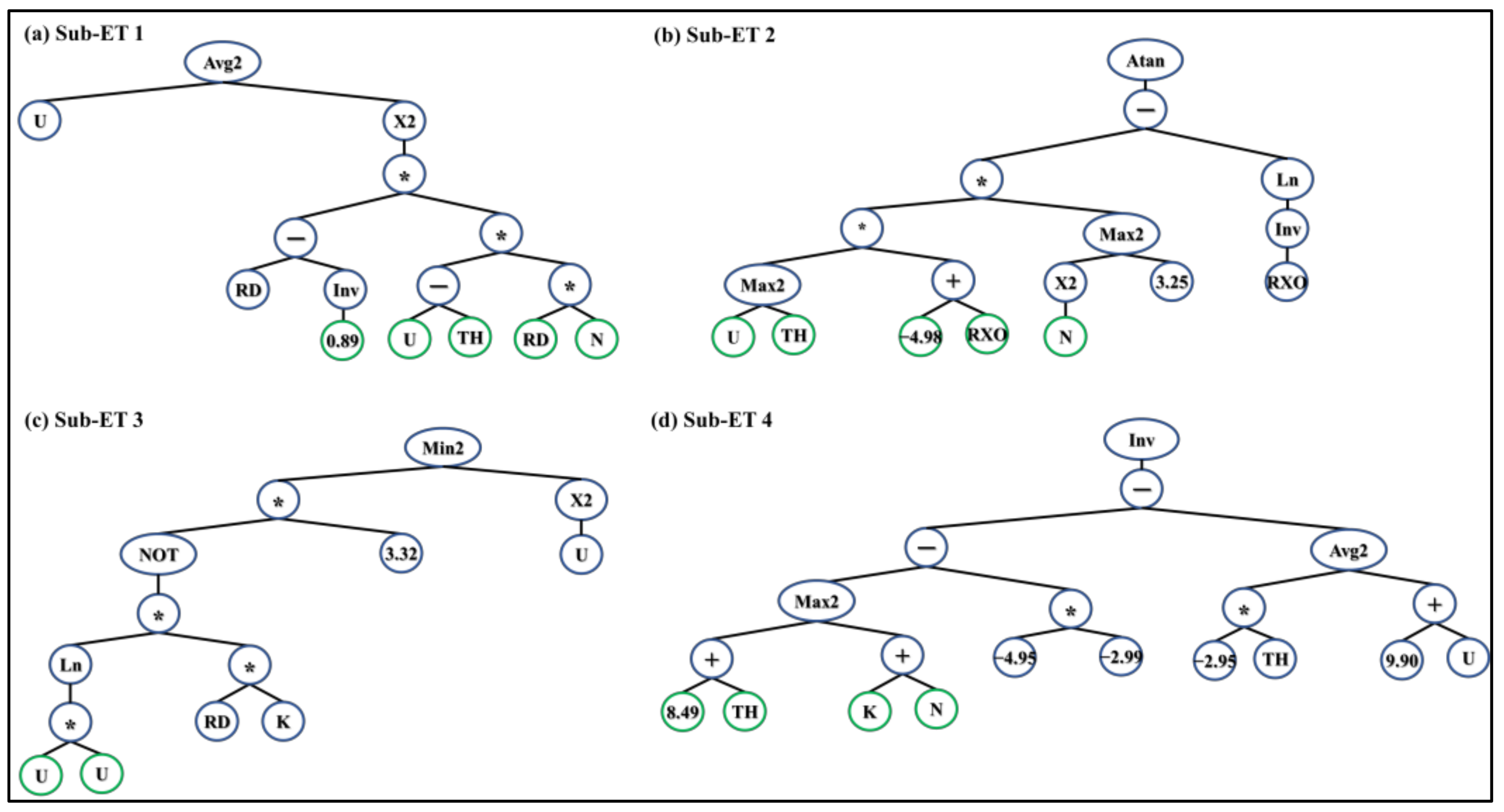
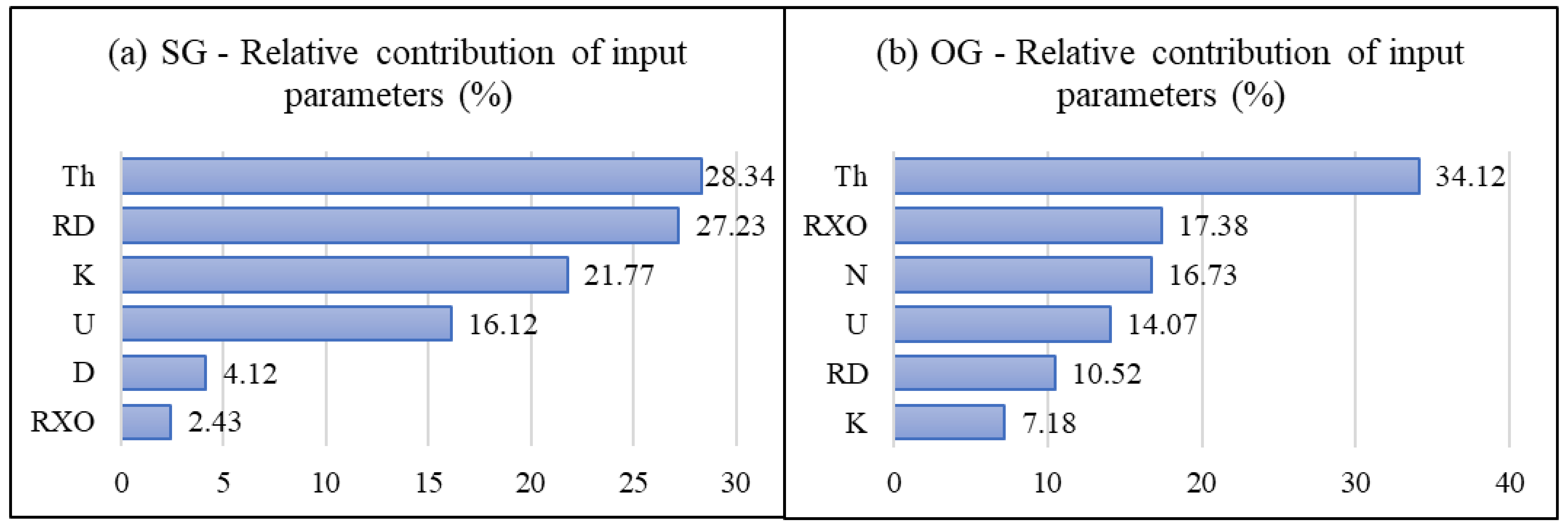
• The results from GEP modelling show that the fracture density prediction between SG and OG rock bodies has no significant difference regarding the well-log responses. The significant parameters for SG are K, TH, U, RD, RXO, and D, while the significant parameters for OG are K, TH, U, RD, RXO, and N.
• The results of this study show that spectral gamma ray, composed of K, TH, and U, is one of the critical parameters for FD predictions in a metamorphic rock body. The results confirmed and were consistent with the previous studies that GR alone did not contribute as much to fracture detection. However, it is one of the most helpful well-log parameters for lithology identification.
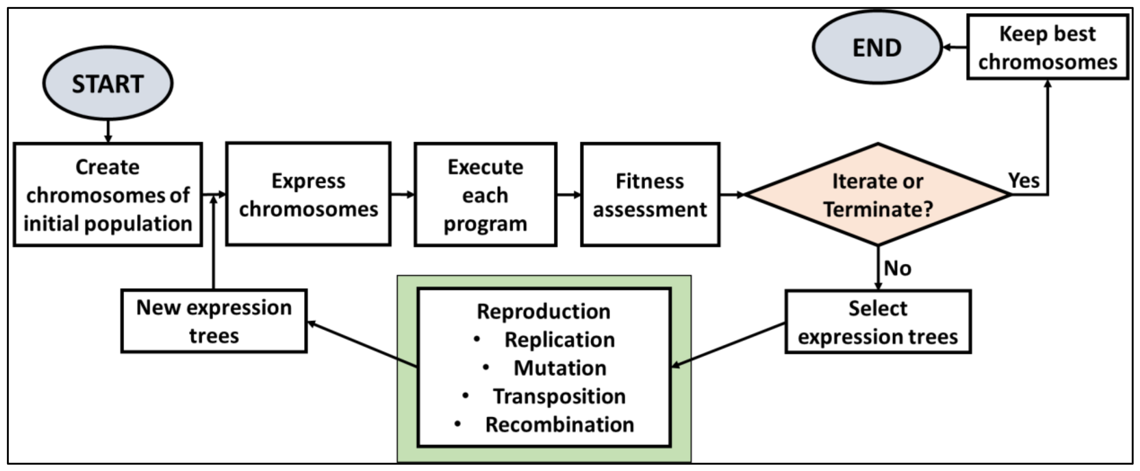
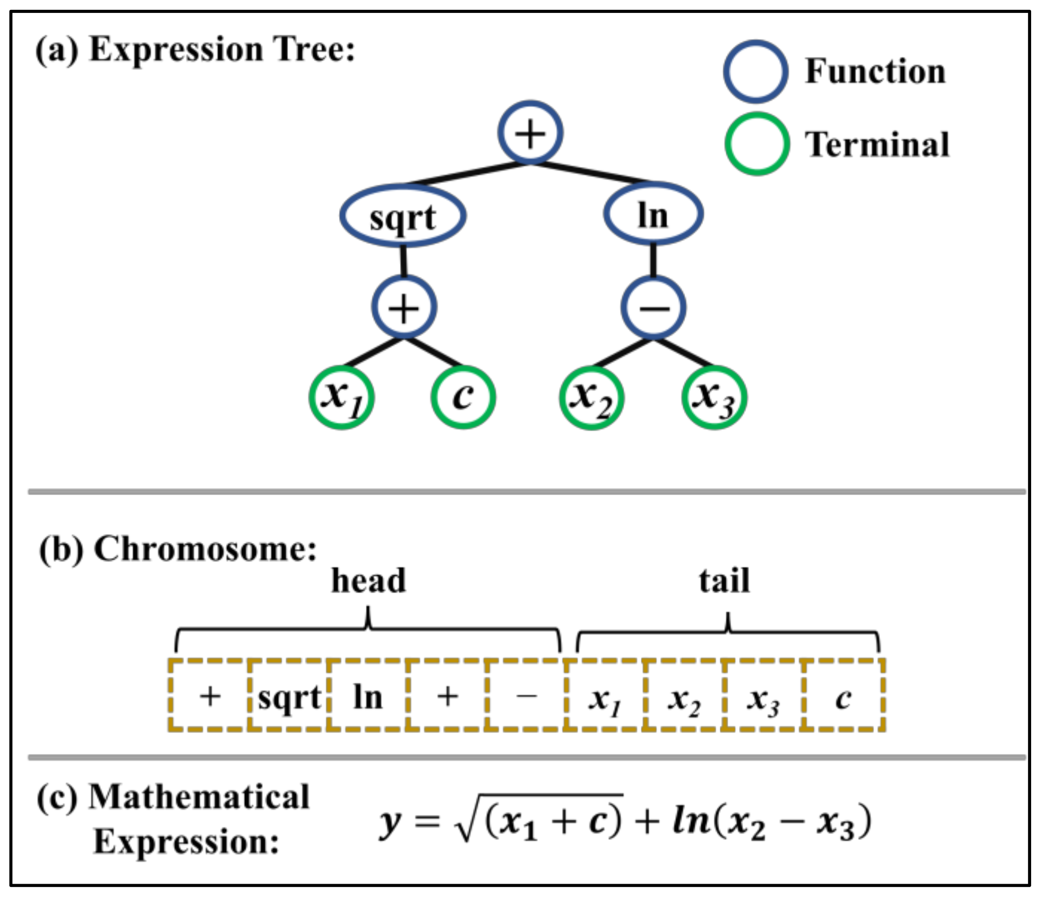
• GEP modelling could be used to predict FD in cases where image logs and core samples are unavailable. The GEP method has been proven helpful in this prediction by using only conventional well-logs as input data. This shows that the nonlinear method could solve a nonlinear and complex problem.
• The prediction of FD to wells without image logs can be validated by comparing the well-log pattern of wells with image logs. In this case, an analysis of all fracture indications from conventional well-logs was carried out, and the results were consistent throughout all wells, either with or without image logs.
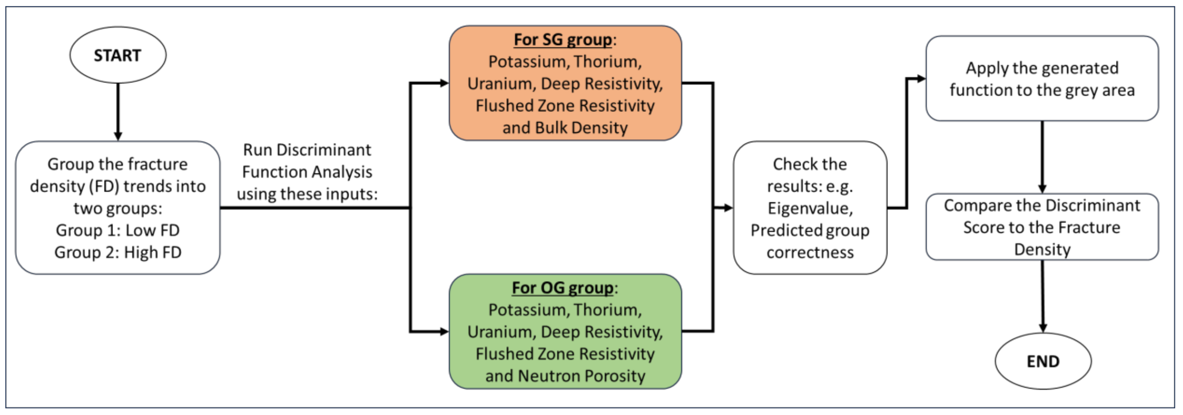
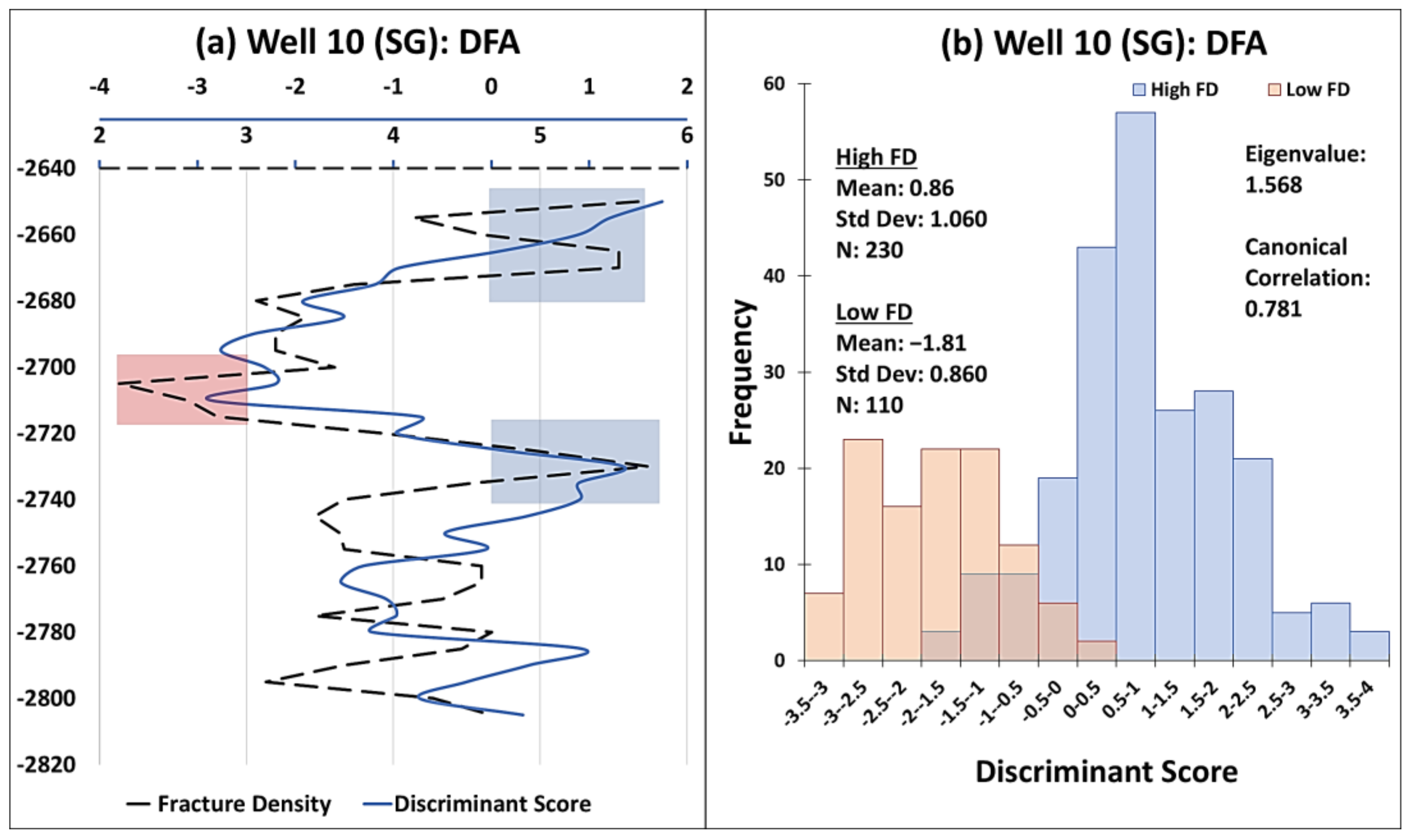
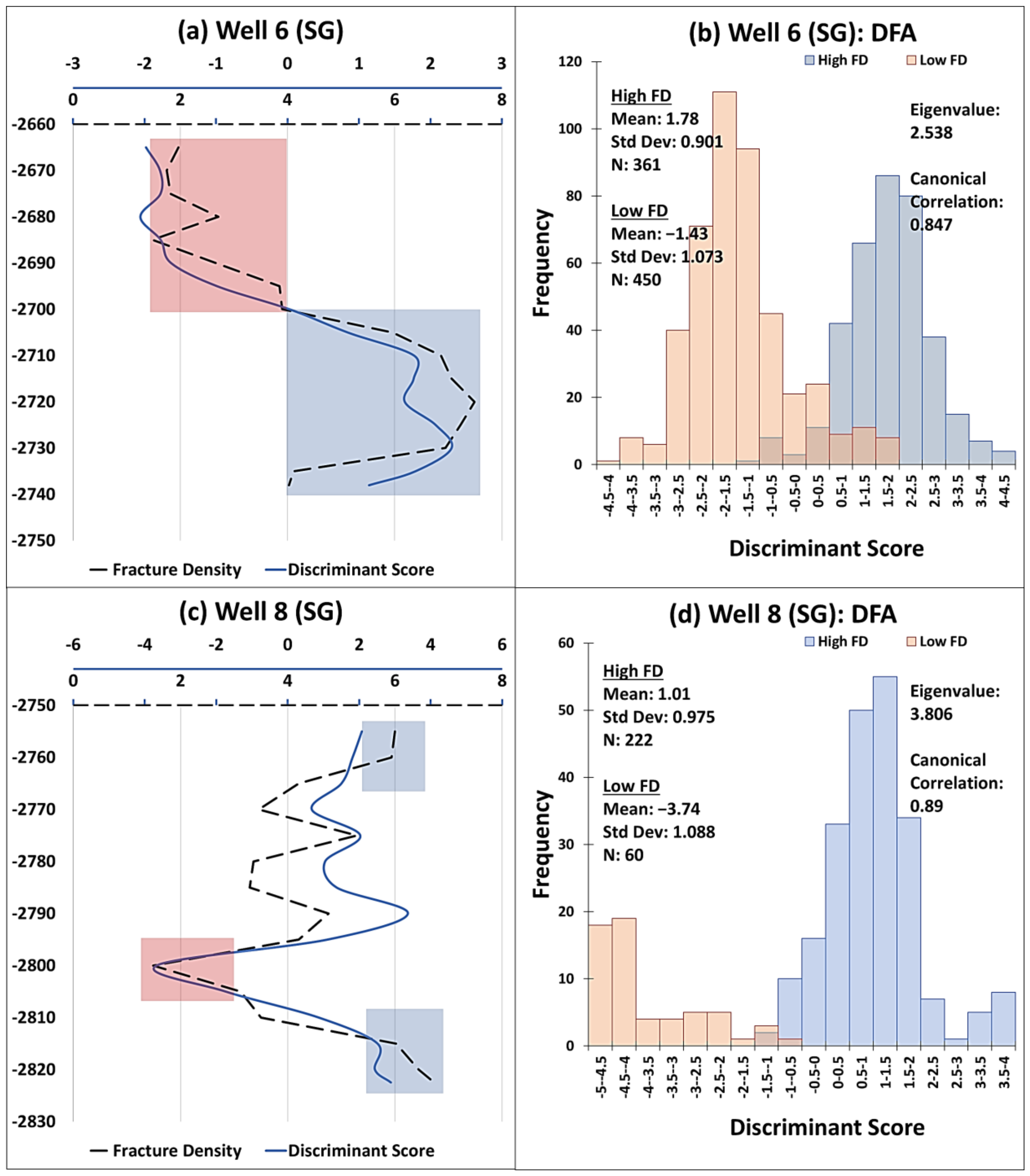
• The study also proposes a method to validate the FD predictions using the statistical analysis method of discriminant function analysis (DFA). The results from GEP modelling were used as inputs for the DFA, and the results show the consistency of the results between wells with image logs and wells without image logs in terms of patterns and trends.
• There are limitations to this study. The study used samples from the basement metamorphic rocks. Although the application of the GEP method seemed to work in the case of this study, the generated functions and methods cannot be generalized for all other fractures since each fracture and rock acts differently. However, this study provides evidence that in the case of two different gneisses, predicting FD without core samples and image logs but using conventional well logs is possible.
• There are many advanced methods that have been developed that utilise the advantages of different machine learning methods. This study proposes that an extended study could be carried out in a similar manner by employing these different methods. However, it is also safe to say that although these model predictions could work, these methods could not replace geophysical analysis, especially image logs.

References

1. Yang, H.; Pan, H.; Wu, A.; Luo, M.; Konaté, A.A.; Meng, Q. Application of well logs integration and wavelet transform to improve fracture zones detection in metamorphic rocks. J. Pet. Sci. Eng. 2017, 157, 716–723. [Google Scholar] [CrossRef]
2. Barthélémy, J.F.; Guiton, M.L.; Daniel, J.M. Estimates of fracture density and uncertainties from well data. Int. J. Rock Mech. Min. Sci. 2009, 46, 590–603. [Google Scholar] [CrossRef]
3. Rashid, F.; Hussein, D.; Lawrence, J.A.; Khanaqa, P. Characterization and impact on reservoir quality of fractures in the Cretaceous Qamchuqa Formation, Zagros folded belt. Mar. Pet. Geol. 2020, 113, 104117. [Google Scholar] [CrossRef]
4. Hu, S.; Wang, X.; Wang, J.; Wang, L. Quantitative evaluation of fracture porosity from dual laterlog based on deep learning method. Energy Geosci. 2023, 4, 100064. [Google Scholar] [CrossRef]
5. Khoshbakht, F.; Rasaie, M.R.; Shekarifard, A. Investigating induction log response in the presence of natural fractures. J. Pet. Sci. Eng. 2016, 145, 357–369. [Google Scholar] [CrossRef]
6. Aghli, G.; Moussavi-Harami, R.; Mohammadian, R. Reservoir heterogeneity and fracture parameter determination using electrical image logs and petrophysical data (a case study, carbonate Asmari Formation, Zagros Basin, SW Iran). Pet. Sci. 2020, 17, 51–69. [Google Scholar] [CrossRef]
7. Pham, C.; Zhuang, L.; Yeom, S.; Shin, H.S. Automatic fracture characterization in CT images of rocks using an ensemble deep learning approach. Int. J. Rock Mech. Min. Sci. 2023, 170, 105531. [Google Scholar] [CrossRef]
8. Cappuccio, F.; Toy, V.G.; Mills, S.; Adam, L. Three-dimensional separation and characterization of fractures in X-ray computed tomographic images of rocks. Front. Earth Sci. 2020, 8, 529263. [Google Scholar] [CrossRef]
9. Zhuo, R.; Ma, X.; Zhang, S.; Ma, J.; Xiang, Y.; Sun, H. Classification and assessment of core fractures in a post-fracturing conglomerate reservoir using the AHP–FCE method. Energies 2022, 16, 418. [Google Scholar] [CrossRef]
10. Dong, T.; Zhou, J.; Yan, Z.; Wu, Y.; Mao, T. Study on voids and seepage characteristics within rock fracture after shear dislocation viewing from CT test and numerical modeling. Appl. Sci. 2024, 14, 1013. [Google Scholar] [CrossRef]
11. Liu, L.; Yao, J.; Sun, H.; Zhang, L.; Zhang, K. Digital rock analysis on the influence of coarse micro-fractures on petrophysical properties in tight sandstone reservoirs. Appl. Sci. 2023, 13, 5237. [Google Scholar] [CrossRef]
12. Ameen, M.S.; MacPherson, K.; Al-Marhoon, M.I.; Rahim, Z. Diverse fracture properties and their impact on performance in conventional and tight-gas reservoirs, Saudi Arabia: The Unayzah, South Haradh case study. AAPG Bull. 2012, 96, 459–492. [Google Scholar] [CrossRef]
13. Lyu, W.; Zeng, L.; Liu, Z.; Liu, G.; Zu, K. Fracture responses of conventional logs in tight-oil sandstones: A case study of the Upper Triassic Yanchang Formation in southwest Ordos Basin, China. AAPG Bull. 2016, 100, 1399–1417. [Google Scholar] [CrossRef]
14. Bagheri, H.; Falahat, R. Fracture permeability estimation utilizing conventional well logs and flow zone indicator. Pet. Res. 2022, 7, 357–365. [Google Scholar] [CrossRef]
15. Qiu, X.; Tan, C.; Lu, Y.; Yin, S. Evaluation of fractures using conventional and FMI logs, and 3D seismic interpretation in continental tight sandstone reservoir. Open Geosci. 2022, 14, 530–543. [Google Scholar] [CrossRef]
16. Aghli, G.; Moussavi-Harami, R.; Tokhmechi, B. Integration of sonic and resistivity conventional logs for identification of fracture parameters in the carbonate reservoirs (A case study, Carbonate Asmari Formation, Zagros Basin, SW Iran). J. Pet. Sci. Eng. 2020, 186, 106728. [Google Scholar] [CrossRef]
17. Tabasi, S.; Tehrani, P.S.; Rajabi, M.; Wood, D.A.; Davoodi, S.; Ghorbani, H.; Mohamadian, N.; Alvar, M.A. Optimized machine learning models for natural fractures prediction using conventional well logs. Fuel 2022, 326, 124952. [Google Scholar] [CrossRef]
18. Gamal, M.; El-Araby, A.A.; El-Barkooky, A.N.; Hassan, A. Detection and characterization of fractures in the Eocene Thebes formation using conventional well logs in October field, Gulf of Suez, Egypt. Egypt. J. Pet. 2022, 31, 1–9. [Google Scholar] [CrossRef]
19. Hussein, H.S. Carbonate fractures from conventional well log data, Kometan Formation, Northern Iraq case study. J. Appl. Geophys. 2022, 206, 104810. [Google Scholar] [CrossRef]
20. Laongsakul, P. Characterization of Reservoir Fractures Using Conventional Geophysical Logging. Doctoral Dissertation, Prince of Songkla University Faculty of Science (Geophysics), Hat Yai, Thailand, 2010. [Google Scholar]
21. Tokhmechi, B.; Memarian, H.; Noubari, H.A.; Moshiri, B. A novel approach proposed for fractured zone detection using petrophysical logs. J. Geophys. Eng. 2009, 6, 365–373. [Google Scholar] [CrossRef]
22. Shalaby, M.R.; Islam, M.A. Fracture detection using conventional well logging in carbonate Matulla Formation, Geisum oil field, southern Gulf of Suez, Egypt. J. Pet. Explor. Prod. Technol. 2017, 7, 977–989. [Google Scholar] [CrossRef]
23. Laongsakul, P.; Dürrast, H. Characterization of reservoir fractures using conventional geophysical logging. Songklanakarin J. Sci. Technol. 2011, 33, 237–246. [Google Scholar]
24. Rashid, M.; Luo, M.; Ashraf, U.; Hussain, W.; Ali, N.; Rahman, N.; Hussain, S.; Aleksandrovich Martyushev, D.; Vo Thanh, H.; Anees, A. Reservoir quality prediction of gas-bearing carbonate sediments in the Qadirpur Field: Insights from advanced machine learning approaches of SOM and cluster analysis. Minerals 2023, 13, 29. [Google Scholar] [CrossRef]
25. Ma, T.; Liu, K.; Su, X.; Chen, P.; Ranjith, P.G.; Martyushev, D.A. Investigation on the Anisotropy of Meso-Mechanical Properties of Shale Rock Using Micro-Indentation. Bull. Eng. Geol. Environ. 2023, 83, 29. [Google Scholar] [CrossRef]
26. Tóth, E.; Hrabovszki, E.; Tóth, T.M. Using geophysical log data to predict the fracture density in a claystone host rock for storing high-level nuclear waste. Acta Geod. Geophys. 2023, 58, 35–51. [Google Scholar] [CrossRef]
27. Sahimi, M.; Hashemi, M. Wavelet identification of the spatial distribution of fractures. Geophys. Res. Lett. 2001, 28, 611–614. [Google Scholar] [CrossRef]
28. Zhang, X.F.; Pan, B.Z.; Wang, F.; Han, X. A study of wavelet transforms applied for fracture identification and fracture density evaluation. Appl. Geophys. 2011, 8, 164–169. [Google Scholar] [CrossRef]
29. Yousef, A.N.; Behzad, T.; Abolghasem, K.R.; Shahram, S.; Kaveh, K.; Amin, J. A combined Parzen-wavelet approach for detection of vuggy zones in fractured carbonate reservoirs using petrophysical logs. J. Pet. Sci. Eng. 2014, 119, 1–7. [Google Scholar] [CrossRef]
30. Tokhmechi, B.; Memarian, H.; Rasouli, V.; Noubari, H.A.; Moshiri, B. Fracture detection from water saturation log data using a Fourier–wavelet approach. J. Pet. Sci. Eng. 2009, 69, 129–138. [Google Scholar] [CrossRef]
31. Taherdangkoo, R.; Abdideh, M. Application of wavelet transform to detect fractured zones using conventional well logs data (Case study: Southwest of Iran). Int. J. Pet. Eng. 2016, 2, 125–139. [Google Scholar] [CrossRef]
32. Martyushev, D.A.; Yurikov, A. Evaluation of Opening of Fractures in the Logovskoye Carbonate Reservoir, Perm Krai, Russia. Pet. Res. 2021, 6, 137–143. [Google Scholar] [CrossRef]
33. Xue, Y.; Cheng, L.; Mou, J.; Zhao, W. A new fracture prediction method by combining genetic algorithm with neural network in low-permeability reservoirs. J. Pet. Sci. Eng. 2014, 121, 159–166. [Google Scholar] [CrossRef]
34. Pei, J.; Zhang, Y. Prediction of Reservoir Fracture Parameters Based on the Multi-Layer Perceptron Machine-Learning Method: A Case Study of Ordovician and Cambrian Carbonate Rocks in Nanpu Sag, Bohai Bay Basin, China. Processes 2022, 10, 2445. [Google Scholar] [CrossRef]
35. Afrasiabian, B.; Eftekhari, M. Prediction of mode I fracture toughness of rock using linear multiple regression and gene expression programming. J. Rock Mech. Geotech. Eng. 2022, 14, 1421–1432. [Google Scholar] [CrossRef]
36. Ari, D.; Alagoz, B.B. A differential evolutionary chromosomal gene expression programming technique for electronic nose applications. Appl. Soft Comput. 2023, 136, 110093. [Google Scholar] [CrossRef]
37. Aydogan, M.S.; Alacali, S.; Arslan, G. Prediction of moment redistribution capacity in reinforced concrete beams using gene expression programming. Structures 2023, 47, 2209–2219. [Google Scholar] [CrossRef]
38. Chu, H.H.; Khan, M.A.; Javed, M.; Zafar, A.; Khan, M.I.; Alabduljabbar, H.; Qayyum, S. Sustainable use of fly-ash: Use of gene-expression programming (GEP) and multi-expression programming (MEP) for forecasting the compressive strength geopolymer concrete. Ain Shams Eng. J. 2021, 12, 3603–3617. [Google Scholar] [CrossRef]
39. Ferreira, C. Gene expression programming: A new adaptive algorithm for solving problems. Complex Syst. 2001, 13, 87–129. [Google Scholar] [CrossRef]
40. Kaushik, V.; Kumar, M. Sustainable gene expression programming model for shear stress prediction in nonprismatic compound channels. Sustain. Energy Technol. Assess. 2023, 57, 103229. [Google Scholar] [CrossRef]
41. Tari, G.; Dövényi, P.; Dunkl, I.; Horváth, F.; Lenkey, L.; Stefanescu, M.; Szafian, P.; Tóth, T. Lithospheric structure of the Pannonian basin derived from seismic, gravity and geothermal data. Geol. Soc. Lond. Spec. Publ. 1999, 156, 215–250. [Google Scholar] [CrossRef]
42. Horváth, F.; Musitz, B.; Balázs, A.; Végh, A.; Uhrin, A.; Nádor, A.; Koroknai, B.; Pap, N.; Tóth, T.; Wórum, G. Evolution of the Pannonian basin and its geothermal resources. Geothermics 2015, 53, 328–352. [Google Scholar] [CrossRef]
43. Tóth, T.M.; Fiser-Nagy, Á.; Kondor, H.; Molnár, L.; Schubert, F.; Vargáné Tóth, I.; Zachar, J. The Metamorphic Basement of the Great Hungarian Plain: From Zwischengebirge Towards A Variegated Mosaic. Földtani Közlöny 2021, 151, 3–26, (in Hungarian with English abstract). [Google Scholar] [CrossRef]
44. Molnár, L.; Tóth, T.M.; Schubert, F. Structural controls on petroleum migration and entrapment within the faulted basement blocks of Szeghalom Dome (Pannonian Basin, SE Hungary). Geol. Croat. 2015, 68, 247–259. [Google Scholar] [CrossRef]
45. Juhász, A.; Tóth, T.M.; Ramseyer, K.; Matter, A. Connected fluid evolution in the fractured crystalline basement and overlying sediments, Pannonian Basin, SE Hungary. Chem. Geol. 2002, 182, 91–120. [Google Scholar] [CrossRef]
46. Schubert, F.; Diamond, L.W.; Tóth, T.M. Fluid-inclusion evidence of petroleum migration through a buried metamorphic dome in the Pannonian Basin, Hungary. Chem. Geol. 2007, 244, 357–381. [Google Scholar] [CrossRef]
47. Kovács, Z.; Zilahi-Sebess, L. Evaluation of the trends of secondary and tertiary hydrocarbon migration processes based on oil density–reservoir depths relationship in Hungary. Cent. Eur. Geol. 2018, 61, 16–33. [Google Scholar] [CrossRef]
48. Selmeczi, I. Hydrocarbon Exploration Areas in Hungary–Bihar. In Hydrocarbons in Hungary; Kovács, Z., Ed.; Hungarian Energy and Public Utility Regulatory Authority: Budapest, Hungary, 2018; pp. 165–178. [Google Scholar]
49. Koroknai, B.; Wórum, G.; Tóth, T.; Koroknai, Z.; Fekete-Németh, V.; Kovács, G. Geological deformations in the Pannonian Basin during the neotectonic phase: New insights from the latest regional mapping in Hungary. Earth-Sci. Rev. 2020, 211, 103411. [Google Scholar] [CrossRef]
50. Molnár, L.; Vásárhelyi, B.; Tóth, T.M.; Schubert, F. Integrated petrographic–rock mechanic borecore study from the metamorphic basement of the Pannonian Basin, Hungary. Open Geosci. 2015, 7, 20150004. [Google Scholar] [CrossRef]
51. Tóth, T.M.; Molnár, L.; Körmös, S.; Czirbus, N.; Schubert, F. Localisation of Ancient Migration Pathways inside a Fractured Metamorphic Hydrocarbon Reservoir in South-East Hungary. Appl. Sci. 2020, 10, 7321. [Google Scholar] [CrossRef]
52. Tóth, T.M.; Zachar, J. Petrology and deformation history of the metamorphic basement in the Mezősas-Furta crystalline high (SE Hungary). Acta Geol. Hung. 2006, 49, 165–188. [Google Scholar] [CrossRef]
53. Hasan, M.L.; Tóth, T.M. Localization of potential migration pathways inside a fractured metamorphic hydrocarbon reservoir using well log evaluation (Mezősas field, Pannonian Basin). Geoenergy Sci. Eng. 2023, 225, 211710. [Google Scholar] [CrossRef]
54. Tóth, T.M.; Schubert, F. Evolution of the arc-derived orthogneiss recorded in exotic xenoliths of the Koros Complex (Tisza Megaunit, SE Hungary). J. Geosci. 2018, 63, 21–46. [Google Scholar] [CrossRef]
55. Baouche, R.; Sen, S.; Chaouchi, R.; Ganguli, S.S. Modeling In-Situ Tectonic Stress State and Maximum Horizontal Stress Azimuth in the Central Algerian Sahara—A Geomechanical Study from El Agreb, El Gassi and Hassi Messaoud Fields. J. Nat. Gas. Sci. Eng. 2021, 88, 103831. [Google Scholar] [CrossRef]
56. Lai, J.; Pang, X.; Xiao, Q.; Shi, Y.; Zhang, H.; Zhao, T.; Chen, J.; Wang, G.; Qin, Z. Prediction of Reservoir Quality in Carbonates via Porosity Spectrum from Image Logs. J. Pet. Sci. Eng. 2019, 173, 197–208. [Google Scholar] [CrossRef]
57. Lai, J.; Wang, G.; Wang, S.; Cao, J.-T.; Li, M.; Pang, X.; Han, C.; Fan, X.; Yang, L.; He, Z.; et al. A Review on the Applications of Image Logs in Structural Analysis and Sedimentary Characterization. Mar. Pet. Geol. 2018, 95, 139–166. [Google Scholar] [CrossRef]
58. Khoshbakht, F.; Memarian, H.; Mohammadnia, M. Comparison of Asmari, Pabdeh and Gurpi Formation’s Fractures, Derived from Image Log. J. Pet. Sci. Eng. 2009, 67, 65–74. [Google Scholar] [CrossRef]
59. Nian, T.; Wang, G.; Xiao, C.; Zhou, L.; Deng, L.; Li, R. The in Situ Stress Determination from Borehole Image Logs in the Kuqa Depression. J. Nat. Gas Sci. Eng. 2016, 34, 1077–1084. [Google Scholar] [CrossRef]
60. Egbue, O.; Kellogg, J.; Aguirre, H.; Torres, C. Evolution of the Stress and Strain Fields in the Eastern Cordillera, Colombia. J. Struct. Geol. 2014, 58, 8–21. [Google Scholar] [CrossRef]
61. Aleardi, M.; Mazzotti, A.; Tognarelli, A.; Ciuffi, S.; Casini, M. Seismic and Well Log Characterization of Fractures for Geothermal Exploration in Hard Rocks. Geophys. J. Int. 2015, 203, 270–283. [Google Scholar] [CrossRef]
62. Algaifi, H.A.; Alqarni, A.S.; Alyousef, R.; Bakar, S.A.; Ibrahim, M.W.; Shahidan, S.; Ibrahim, M.; Salami, B.A. Mathematical prediction of the compressive strength of bacterial concrete using gene expression programming. Ain Shams Eng. J. 2021, 12, 3629–3639. [Google Scholar] [CrossRef]
63. Jafari, S.; Mahini, S.S. Lightweight Concrete Design Using Gene Expression Programing. Constr. Build. Mater. 2017, 139, 93–100. [Google Scholar] [CrossRef]
64. Beheshti Aval, S.B.; Ketabdari, H.; Asil Gharebaghi, S. Estimating Shear Strength of Short Rectangular Reinforced Concrete Columns Using Nonlinear Regression and Gene Expression Programming. Structures 2017, 12, 13–23. [Google Scholar] [CrossRef]
65. Mahmoodzadeh, A.; Nejati, H.R. An optimized equation based on the gene expression programming method for estimating tunnel construction costs considering a variety of variables and indexes. Appl. Soft Comput. 2023, 147, 110749. [Google Scholar] [CrossRef]
66. Zhang, R.; Xue, X.; Deng, C. Investigation of motion characteristics of catastrophic landslide using material point method and gene expression programming. Int. J. Rock Mech. Min. Sci. 2023, 170, 105507. [Google Scholar] [CrossRef]
67. Alzara, M.; Rehman, M.F.; Farooq, F.; Ali, M.; Beshr, A.A.; Yosri, A.M.; El Sayed, S.A. Prediction of building energy performance using mathematical gene-expression programming for a selected region of dry-summer climate. Eng. Appl. Artif. Intell. 2023, 126, 106958. [Google Scholar] [CrossRef]
68. Taleshi, M.M.; Tajik, N.; Mahmoudian, A.; Yekrangnia, M. Prediction of Pull-out Behavior of Timber Glued-in Glass Fiber Reinforced Polymer and Steel Rods under Various Environmental Conditions Based on ANN and GEP Models. Case Stud. Constr. Mater. 2024, 20, e02842. [Google Scholar] [CrossRef]
69. Waqas, H.A.; Bahrami, A.; Sahil, M.; Poshad Khan, A.; Ejaz, A.; Shafique, T.; Tariq, Z.; Ahmad, S.; Özkılıç, Y.O. Performance Prediction of Hybrid Bamboo-Reinforced Concrete Beams Using Gene Expression Programming for Sustainable Construction. Materials 2023, 16, 6788. [Google Scholar] [CrossRef] [PubMed]
70. Leon, L.P.; Gay, D. Gene Expression Programming for Evaluation of Aggregate Angularity Effects on Permanent Deformation of Asphalt Mixtures. Constr. Build. Mater. 2019, 211, 470–478. [Google Scholar] [CrossRef]
71. Peng, H.; Li, L.; Mei, C.; Deng, C.; Yue, X.; Wu, Z. Gene expression programming with dual strategies and neighborhood search for symbolic regression problems. Appl. Soft Comput. 2023, 145, 110616. [Google Scholar] [CrossRef]
72. Zhu, Y.-J.; Nie, X.; Ma, H.; Su, L.-C. Prediction Model for Load Effective Distribution Width of Slab in Composite Box Girders Using Gene Expression Programming. Eng. Struct. 2022, 255, 113930. [Google Scholar] [CrossRef]
73. Murad, Y.; Tarawneh, A.; Arar, F.; Al-Zu’bi, A.; Al-Ghwairi, A.; Al-Jaafreh, A.; Tarawneh, M. Flexural Strength Prediction for Concrete Beams Reinforced with FRP Bars Using Gene Expression Programming. Structures 2021, 33, 3163–3172. [Google Scholar] [CrossRef]
74. Azimi-Pour, M.; Eskandari-Naddaf, H. ANN and GEP Prediction for Simultaneous Effect of Nano and Micro Silica on the Compressive and Flexural Strength of Cement Mortar. Constr. Build. Mater. 2018, 189, 978–992. [Google Scholar] [CrossRef]
75. Shahmansouri, A.A.; Akbarzadeh Bengar, H.; Jahani, E. Predicting Compressive Strength and Electrical Resistivity of Eco-Friendly Concrete Containing Natural Zeolite via GEP Algorithm. Constr. Build. Mater. 2019, 229, 116883. [Google Scholar] [CrossRef]
76. Gholampour, A.; Gandomi, A.H.; Ozbakkaloglu, T. New Formulations for Mechanical Properties of Recycled Aggregate Concrete Using Gene Expression Programming. Constr. Build. Mater. 2017, 130, 122–145. [Google Scholar] [CrossRef]
77. Gandomi, A.H.; Roke, D.A. Assessment of Artificial Neural Network and Genetic Programming as Predictive Tools. Adv. Eng. Softw. 2015, 88, 63–72. [Google Scholar] [CrossRef]
78. Güllü, H. Function Finding via Genetic Expression Programming for Strength and Elastic Properties of Clay Treated with Bottom Ash. Eng. Appl. Artif. Intell. 2014, 35, 143–157. [Google Scholar] [CrossRef]
79. Gandomi, A.H.; Alavi, A.H.; Gandomi, M.; Kazemi, S. Formulation of Shear Strength of Slender RC Beams Using Gene Expression Programming, Part II: With Shear Reinforcement. Measurement 2017, 95, 367–376. [Google Scholar] [CrossRef]
80. Iqbal, M.F.; Liu, Q.; Azim, I.; Zhu, X.; Yang, J.; Javed, M.F.; Rauf, M. Prediction of Mechanical Properties of Green Concrete Incorporating Waste Foundry Sand Based on Gene Expression Programming. J. Hazard. Mater. 2020, 384, 121322. [Google Scholar] [CrossRef] [PubMed]
81. Babanajad, S.K.; Gandomi, A.H.; Alavi, A.H. New Prediction Models for Concrete Ultimate Strength under True-Triaxial Stress States: An Evolutionary Approach. Adv. Eng. Softw. 2017, 110, 55–68. [Google Scholar] [CrossRef]
82. Ali Khan, M.A.; Zafar, A.; Akbar, A.; Javed, M.F.; Mosavi, A. Application of Gene Expression Programming (GEP) for the Prediction of Compressive Strength of Geopolymer Concrete. Materials 2021, 14, 1106. [Google Scholar] [CrossRef] [PubMed]
83. Fisher, R.A. The use of multiple measurements in taxonomic problems. Ann. Eugen. 1936, 7, 179–188. [Google Scholar] [CrossRef]
84. Zhang, L.; Bai, G.; Zhao, X.; Zhou, L.; Zhou, S.; Jiang, W.; Wang, Z. Oil-Source Correlation in the Slope of the Qikou Depression in the Bohai Bay Basin with Discriminant Analysis. Mar. Pet. Geol. 2019, 109, 641–657. [Google Scholar] [CrossRef]
85. Konaté, A.A.; Pan, H.; Ma, H.; Cao, X.; Yevenyo Ziggah, Y.; Oloo, M.; Khan, N. Application of Dimensionality Reduction Technique to Improve Geophysical Log Data Classification Performance in Crystalline Rocks. J. Pet. Sci. Eng. 2015, 133, 633–645. [Google Scholar] [CrossRef]
86. EsMAEl, M.; Bagheri, A.; Navid, S.M.; Mansourian, D.; Ayub, E.; Pedram, N.; Martyushev, D.A. An Efficient and Comprehensive Poroelastic Analysis of Hydrocarbon Systems Using Multiple Data Sets through Laboratory Tests and Geophysical Logs: A Case Study in an Iranian Hydrocarbon Reservoir. Carbonates Evaporites 2023, 38, 37. [Google Scholar] [CrossRef]
87. Petrik, A.; Vahle, C.; Gianotten, I.P.; Trøan, L.I.; Rojo, L.; Galbraith, K. Quantitative Characterisation of Fracture Connectivity from High-Resolution Borehole Image Logs. Mar. Pet. Geol. 2023, 155, 106405. [Google Scholar] [CrossRef]
88. Khoshbakht, F.; Azizzadeh, M.; Memarian, H.; Nourozi, G.H.; Moallemi, S.A. Comparison of electrical image log with core in a fractured carbonate reservoir. J. Pet. Sci. Eng. 2012, 86, 289–296. [Google Scholar] [CrossRef]
89. Camanni, G.; Vinci, F.; Tavani, S.; Ferrandino, V.; Mazzoli, S.; Corradetti, A.; Parente, M.; Iannace, A. Fracture density variations within a reservoir-scale normal fault zone: A case study from shallow-water carbonates of southern Italy. J. Struct. Geol. 2021, 151, 104432. [Google Scholar] [CrossRef]
90. Pontes, C.C.; Bezerra, F.H.; Bertotti, G.; La Bruna, V.; Audra, P.; De Waele, J.; Auler, A.S.; Balsamo, F.; De Hoop, S.; Pisani, L. Flow pathways in multiple-direction fold hinges: Implications for fractured and karstified carbonate reservoirs. J. Struct. Geol. 2021, 146, 104324. [Google Scholar] [CrossRef]
91. Ammari, A.; Abbes, C.; Abida, H. Geometric properties and scaling laws of the fracture network of the Ypresian carbonate reservoir in central Tunisia: Examples of Jebels Ousselat and Jebil. J. Afr. Earth Sci. 2022, 196, 104718. [Google Scholar] [CrossRef]
Figure 1. Topographic map of the studied area with interpreted lithology and fault lines from [53]. The number shown on the map is the well number and its location; the isolines indicate the depth below the present surface in metres. Abbreviations: AG—amphibolite, AG2—amphibole–biotite gneiss (not shown in this figure, but lies underneath the AG; more details are shown in Figure 2), SG—sillimanite- and garnet-bearing biotite gneiss, and OG—orthogneiss.
Minerals 14 00366 g001
Figure 2. The cross-section of the studied area is based on the lines shown in the topographic map in Figure 1. The figures show the basement rock sequence with interpreted fault lines responsible for fluid migration [53]. (a) The cross-section from A to B; (b) The cross-section from A to C.
Minerals 14 00366 g002
Figure 3. Typical microphotos of the Mezősas orthogneiss. (a) Polygonal microtexture of feldspar grains (XPL); (b) myrmekitic and perthitic K-feldspar porphyroclast (XPL); (c) idiomorphic zircon crystal (XPL); (d) garnet and clinopyroxene xenocrysts in the quartz–feldspar matrix (PPL); (e) amphibolite xenoliths (the length of the core is ~20 cm); (f) typical texture of a felsic granulite xenolith.
Minerals 14 00366 g003
Figure 4. Typical microphotos of the Mezősas garnet-bearing sillimanite paragneiss. (a) Early kyanite and late sillimanite (XPL); (b) the major foliation is defined by biotite and sillimanite (PPL).
Minerals 14 00366 g004
Figure 5. The workflow used in this study.
Minerals 14 00366 g005
Figure 6. Correlation results of each well-log parameter with fracture density for sillimanite- and garnet-bearing biotite gneiss training data.
Minerals 14 00366 g006
Figure 7. Correlation results of each well-log parameter with fracture density for orthogneiss training data.
Minerals 14 00366 g007
Figure 8. The general gene expression programming workflow (modified from [39]).
Minerals 14 00366 g008
Figure 9. Example of an expression tree and chromosome structure.
Minerals 14 00366 g009
Figure 10. The flowchart of the discriminant function analysis process for the validation of predicted fracture density results.
Minerals 14 00366 g010
Figure 11. Results for fracture density prediction using gene expression programming. Three wells were used as training and testing datasets. The blue line is the measured fracture density values based on image logs. The training dataset was collected from the upper part of each well, indicated by the orange line, and the green line on the lower part of each well is the testing section.
Minerals 14 00366 g011
Figure 12. The predicted and measured fracture density values are plotted for each well, and the R2 values are calculated. All wells show an R2 value above 0.85.
Minerals 14 00366 g012
Figure 13. Expression tree results for the SG rock column generated from GeneXpro Tools 5.0.
Minerals 14 00366 g013
Figure 14. The results of the predicted fracture density of selected wells are shown. These fracture density values were calculated based on Equation (5).
Minerals 14 00366 g014
Figure 15. Results from training wells of OG rock column. The training and testing dataset results from gene expression programming agree with the measured fracture density values from the image logs.
Minerals 14 00366 g015
Figure 16. The R2 results of OG rock column wells with image logs. The R2 values were calculated based on the plot of predicted versus measured fracture density value.
Minerals 14 00366 g016
Figure 17. The expression tree results for the orthogneiss rock column generated by GeneXpro Tools 5.0.
Minerals 14 00366 g017
Figure 18. The fracture density values as predicted by the gene expression programming model; these predictions were made for wells without image logs at the orthogneiss rock column.
Minerals 14 00366 g018
Figure 19. Discriminant function analysis results of one of the SG training wells with image logs: Well 10. The fracture density (FD) values were grouped into two categories, namely, high FD (highlighted in blue) and low FD (highlighted in red).
Minerals 14 00366 g019
Figure 20. The discriminant function analysis results for wells without SG wells’ image logs. (a) fracture density and discriminant score plot of Well 6. The FD data of Well 6 can be easily separated into low and high FD values since the trend is obvious and there is no grey area for this dataset; (b) histogram and results of DFA of Well 6; (c) fracture density and discriminant score plot of Well 8; (d) histogram and results of DFA of Well 8.
Minerals 14 00366 g020
Figure 21. Discriminant function analysis results of one of the OG training wells with image logs (Well 13). The fracture density (FD) values were grouped into two categories, namely, high FD (highlighted in blue) and low FD (highlighted in red).
Minerals 14 00366 g021
Figure 22. The discriminant function analysis results for wells without OG wells’ image logs. (a) Fracture density and discriminant score plot of Well 4; (b) histogram and results of DFA of Well 4; (c) fracture density and discriminant score plot of Well 10; (d) histogram and results of DFA of Well 10.
Minerals 14 00366 g022
Figure 23. Relative contribution of input parameters of both SG and OG.
Minerals 14 00366 g023
Figure 24. Well-to-well correlation of four nearby wells in the studied area: Wells 7, 27, 26, and 13. The black dashed lines are the separation boundaries between two lithologies based on the study from [53] in which the upper part of the well is sillimanite- and garnet-bearing biotite gneiss (SG), and the lower part of the well is orthogneiss (OG). Well 26 only penetrated SG.
Minerals 14 00366 g024
Figure 25. Fracture density frequency plot of (a) sillimanite- and garnet-bearing biotite gneiss (SG) and (b) orthogneiss (OG).
Minerals 14 00366 g025