


Probabilistic Modelling of Geologically Complex Veins of the Barberton Greenstone Complex at Fairview Mine, South Africa

Abstract
1. Introduction
2. Geological Setting
3. Methodology
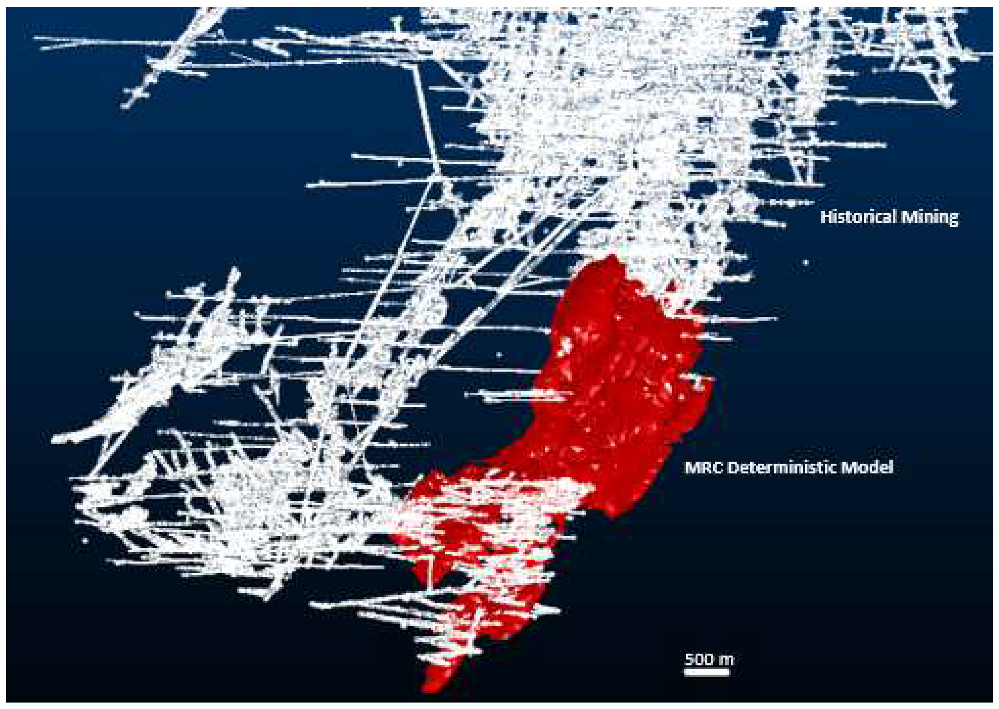
- The initial step employed a deterministic implicit approach based on the MCI to model the overall, large-scale trend of mineralization. This approach generated a simplified solid representation outlining the general shape and boundaries of the ore body, referred to as the ore envelope.
- Following this, a probabilistic approach was applied to model ore shoots within the ore envelope. This involved using an anisotropic inverse distance weighting technique (AIDW), resulting in the delineation of multiple mineralized zones within the deterministic solid.
3.1. Sampling and Interpolation Data
3.2. Deterministic Modeling
3.3. Domaining
3.4. Probabilistic Modelling
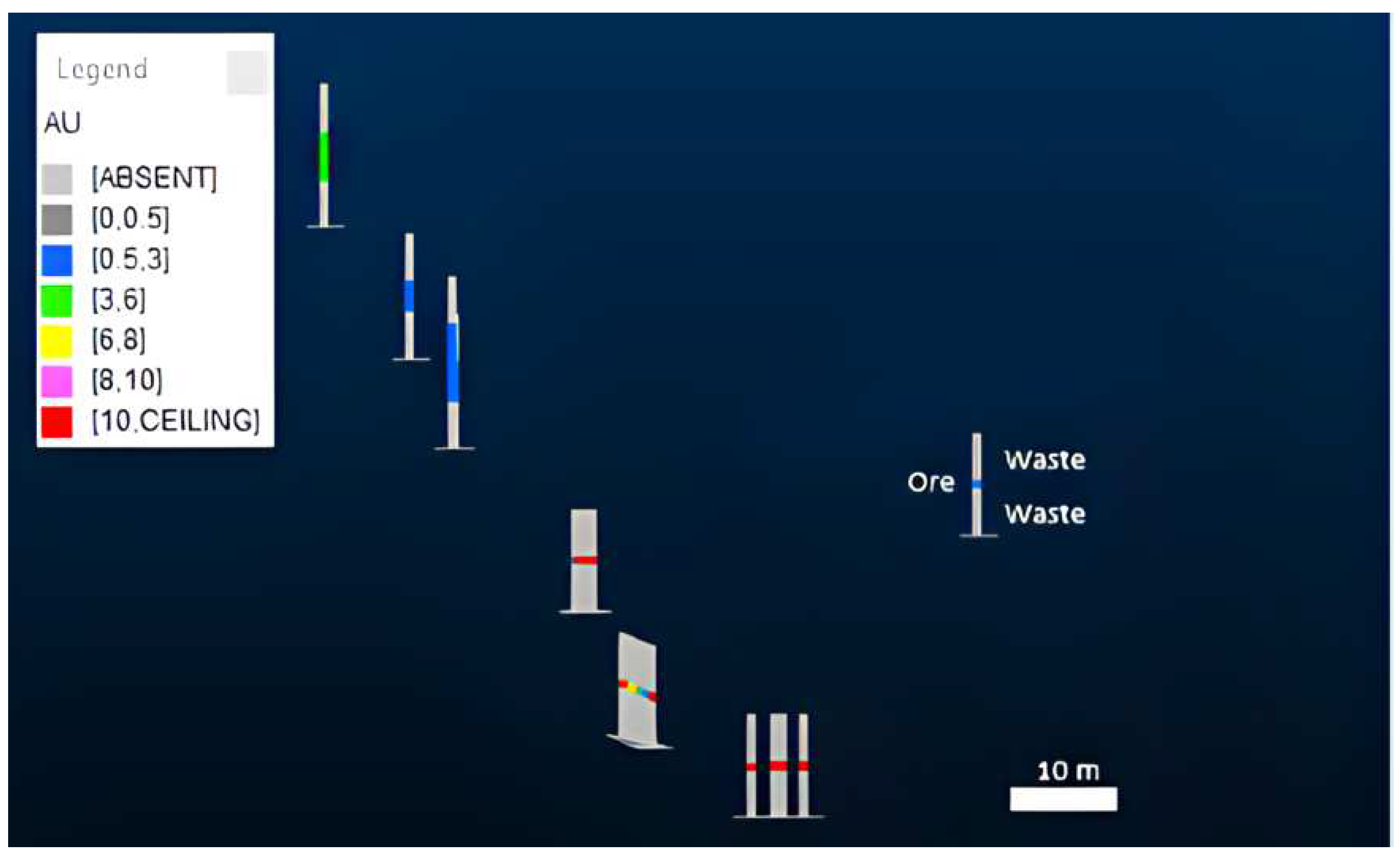
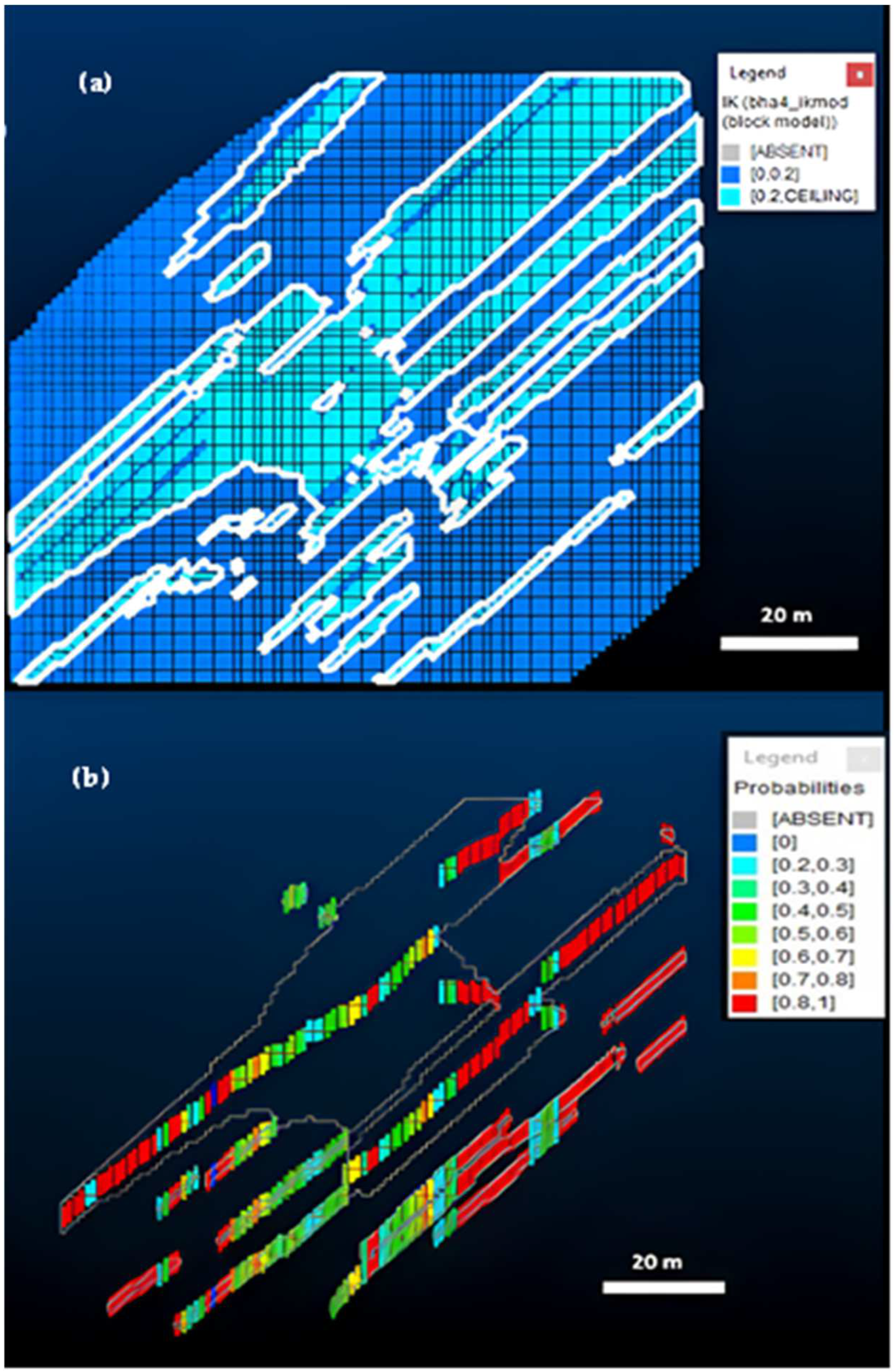
- The two categories (k), mineralized zone (k = 1) and waste (k = 2) were converted to a matrix of indicators, whereby the presence of each category at each known location ui is given an indicator of 1 and its absence is made 0. That is:
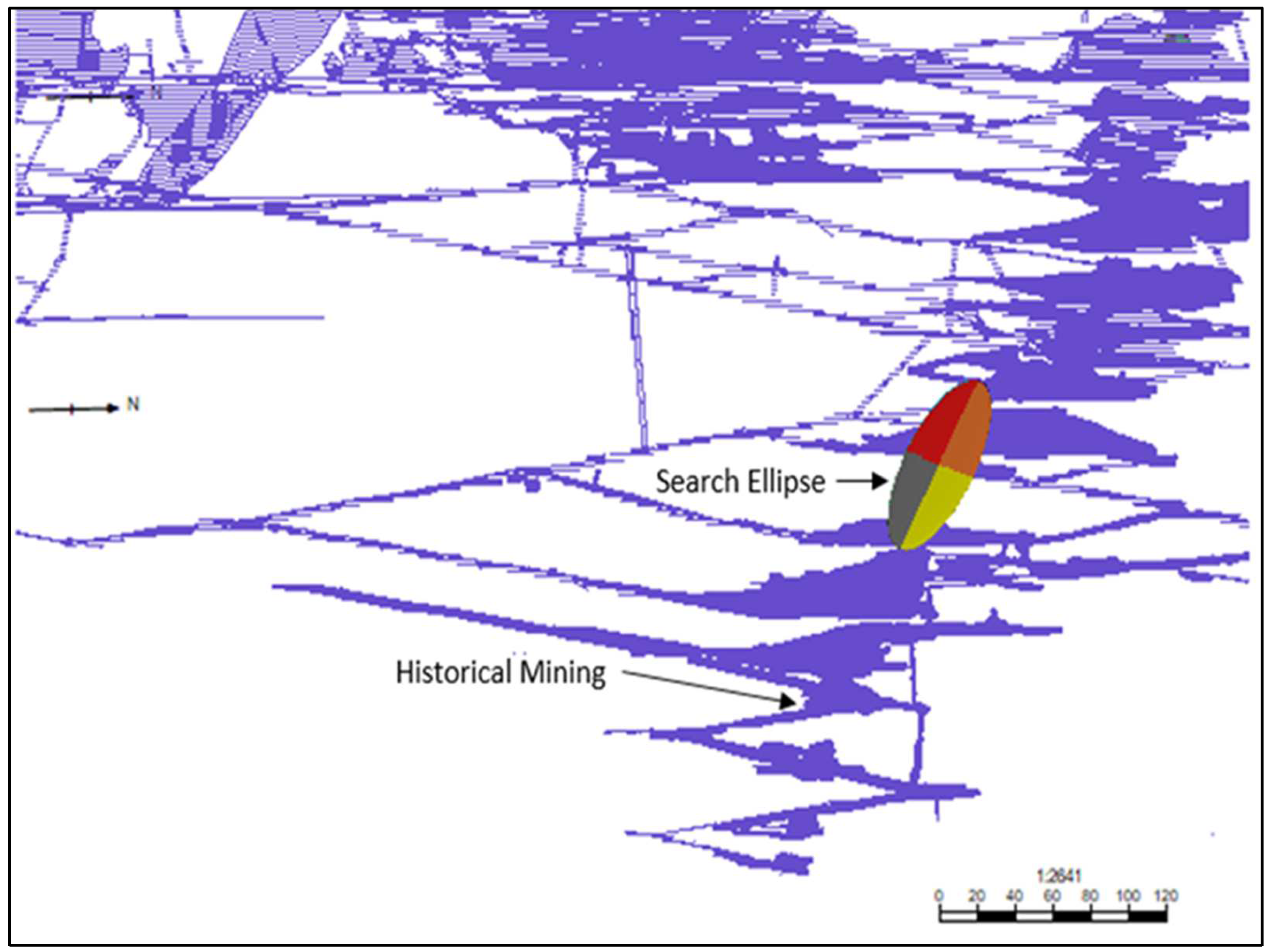
- IDW2 is then used to interpolate estimates of each category’s indicators at unsampled locations based on several search and neighbourhood parameters. The distribution of uncertainty for the categories at each unsampled location is thus directly estimated. In other words, the probability distribution at any unknown location u in each domain will consist of estimated probabilities for each category (), as described by Equations (2) and (3):where wi are IDW2 weights given to the input data and di are the Euclidean distances between the target location and sample points.
- Through a process of iteration, multiple realizations at different probabilities of mineralized zones were visualized and iteratively compared to the existing geological mapping, conceptual models, historic production information, and sample data. The probability level that best fitted the geologic interpretations and database was selected as optimal.
3.5. Grade Interpolation and Validation
4. Results
4.1. Geological Modelling
4.1.1. Deterministic Model
4.1.2. Probabilistic Model
4.2. Resource Modelling
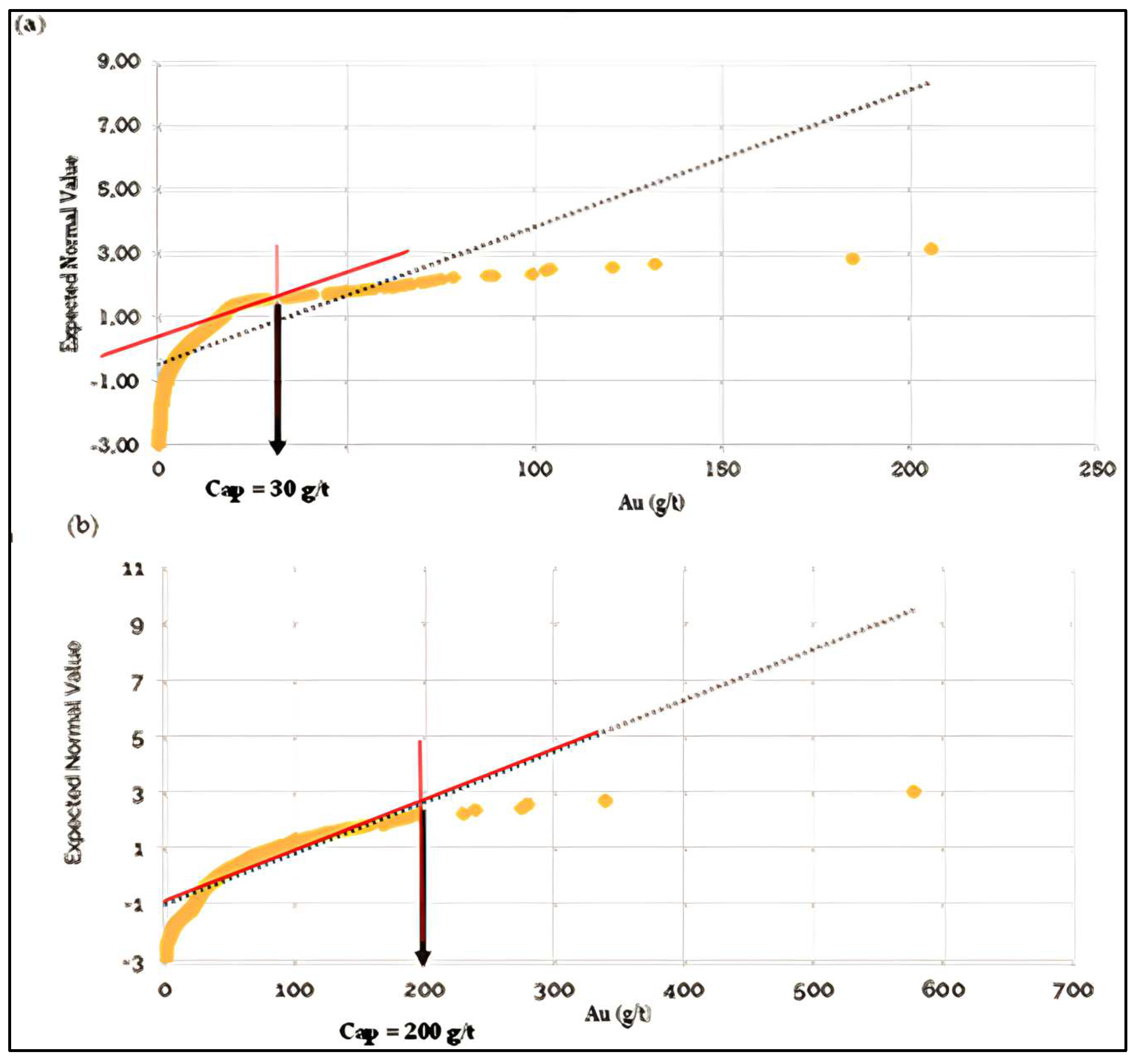
4.2.1. Top Capping
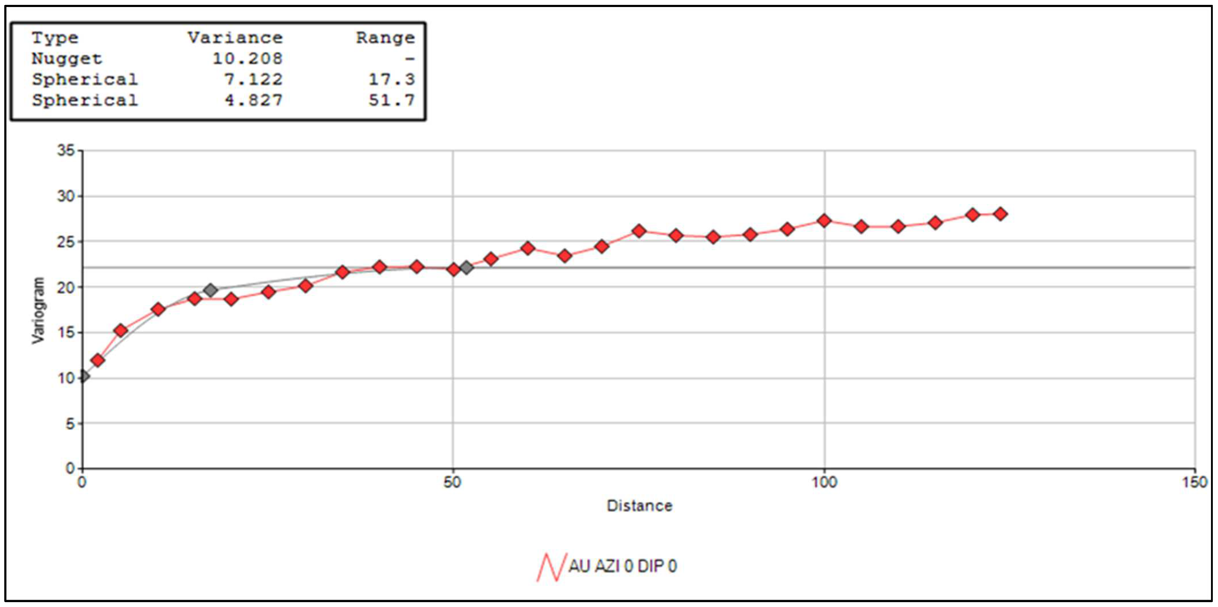
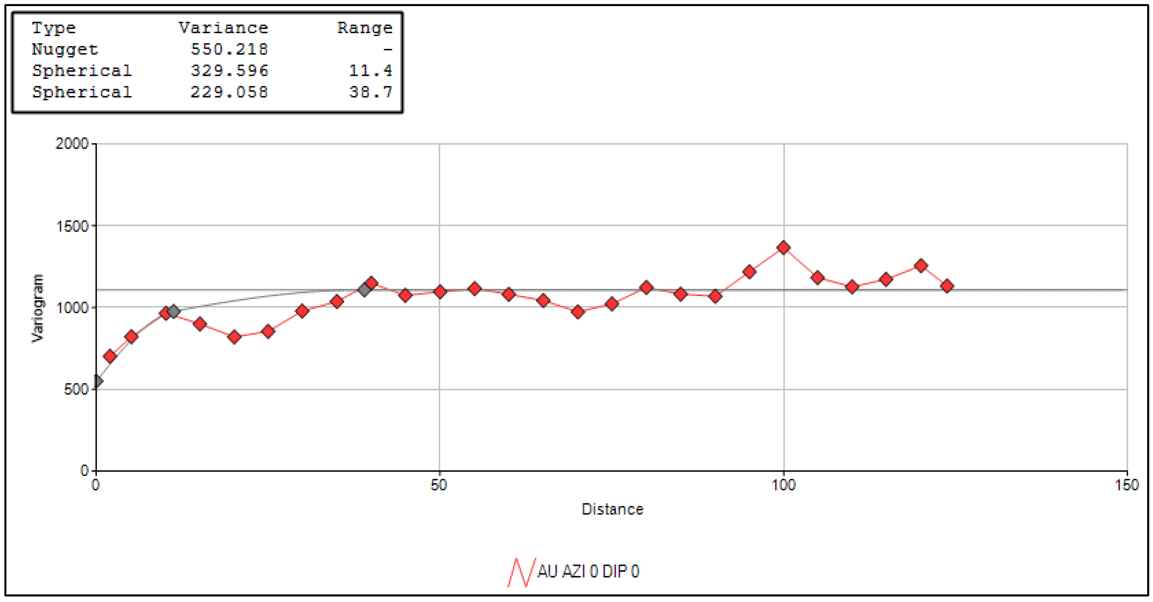
4.2.2. Variography
4.2.3. Grade Interpolation
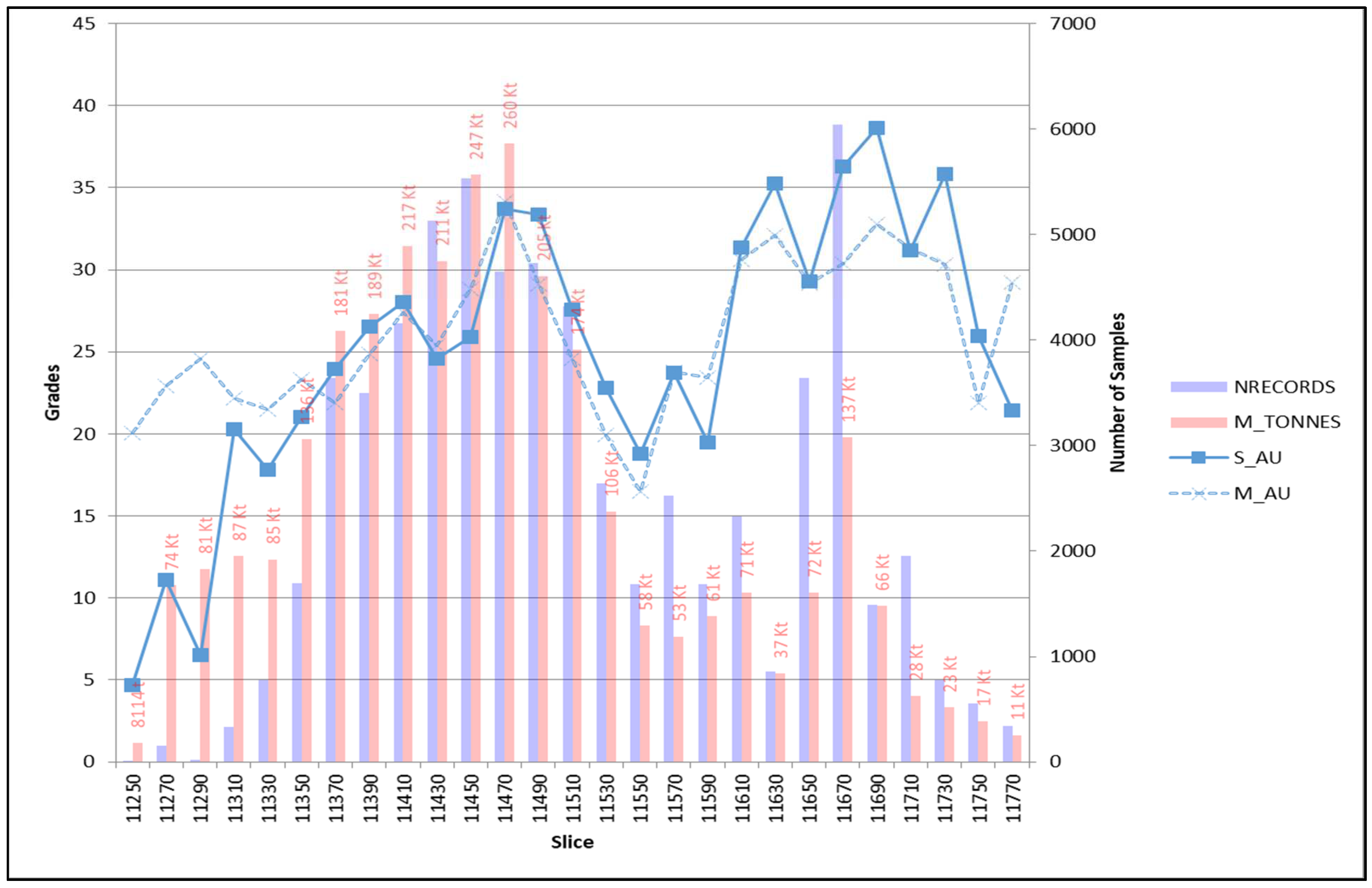
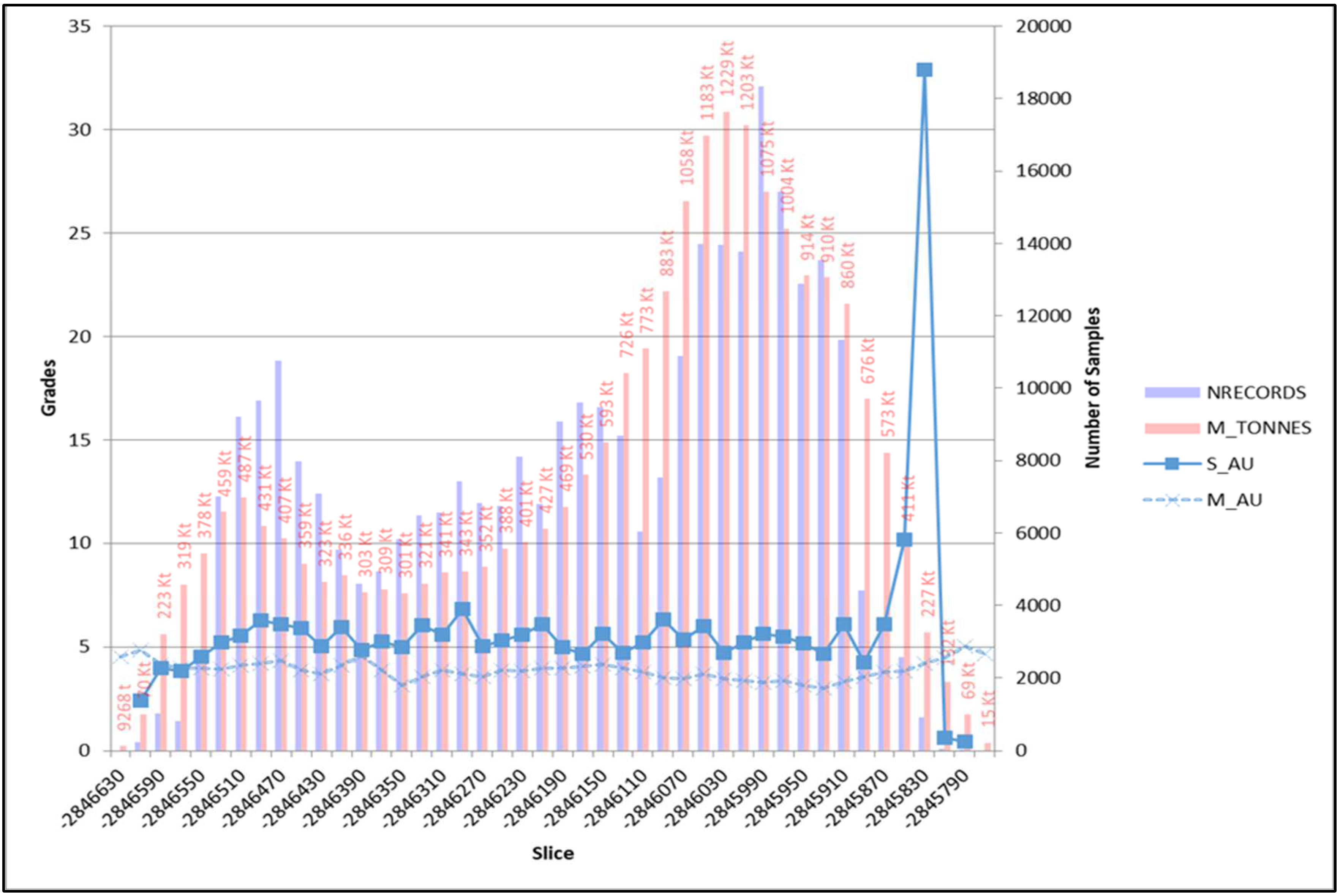
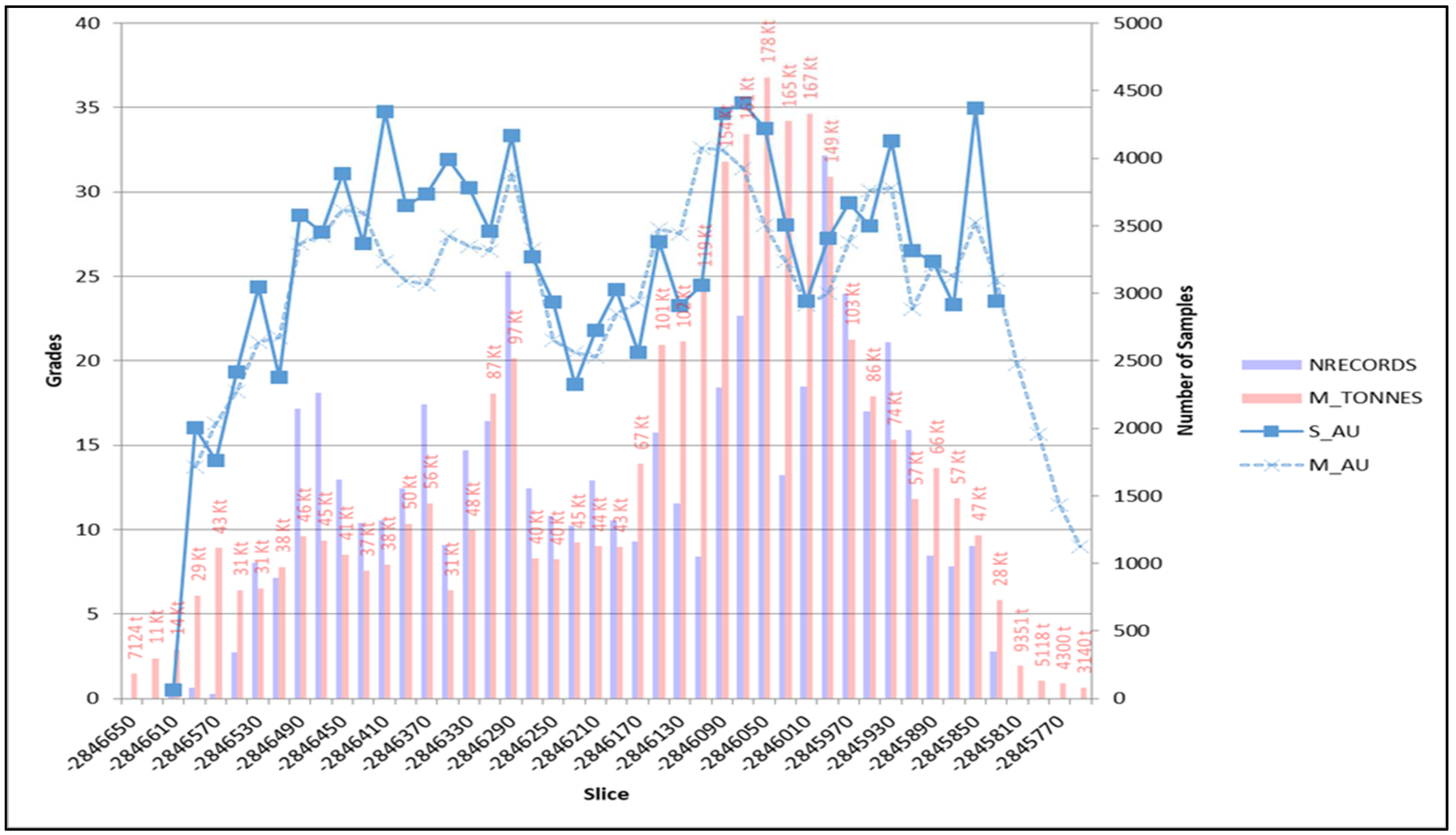
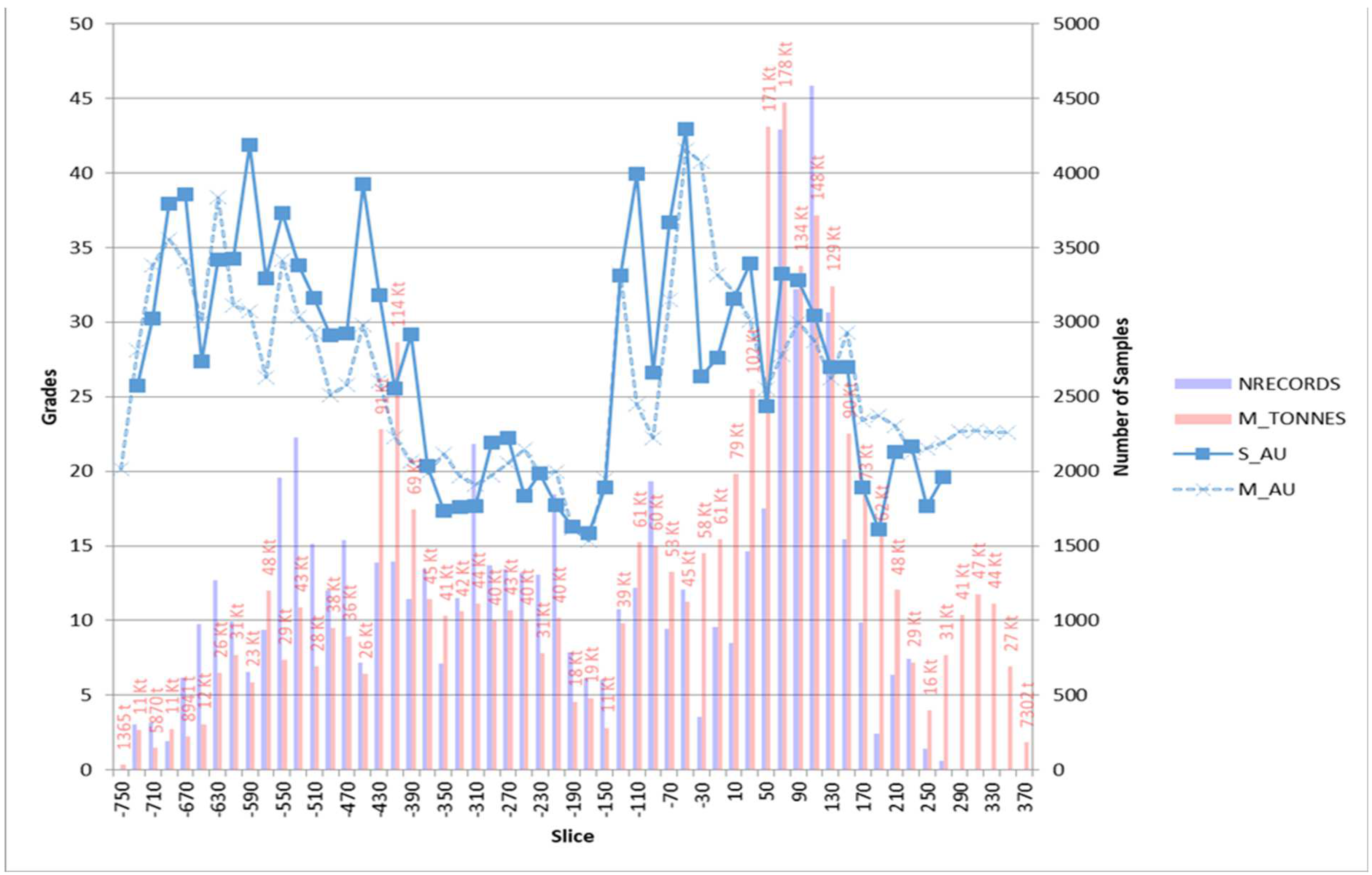
4.2.4. Model Validation
4.2.5. Reasonable Prospect for Eventual Economic Extraction
5. Discussion
Author Contributions
Funding
Data Availability Statement
Acknowledgments
Conflicts of Interest
References
- Sides, E.J. Geological Modelling of Mineral Deposits for Prediction in Mining. Geol. Rundsch. 1997, 86, 342–353. [Google Scholar] [CrossRef]
- Dominy, S.C.; Platten, I.M.; Raine, M.D. Grade and Geological Continuity in High-Nugget Effect Gold-Quartz Reefs: Implications for Resource Estimation and Reporting. Trans. Inst. Min. Metall. Sect. B Appl. Earth Sci. 2003, 112, 239–259. [Google Scholar] [CrossRef]
- Sterk, R. The Konongo Gold Project, Ghana: An Example of How Geology Makes All the Difference to a Resource Estimate. Appl. Earth Sci. 2014, 112, 239–259. [Google Scholar]
- Rossi, M.E.; Strong, T.J.; Brown, P.J. Geological Modelling of Complex Ore Bodies: Combining Deterministic and Probabilistic Models. In Proceedings of the 5th International Seminar on Geology for the Mining Industry, Santiago, Chile, 23–25 August 2017; GEOMIN: Santiago, Chile, 2017. [Google Scholar]
- Ongarbayev, I.; Madani, N. Anisotropic Inverse Distance Weighting Method: An Innovative Technique for Resource Modeling of Vein-Type Deposits. J. Min. Environ. 2022, 13, 957–972. [Google Scholar] [CrossRef]
- Healey, C.M. Geology as a Risk Factor in Project Evaluation: Its Impact on Reserve Estimation. Explor. Min. Geol. 1992, 1, 243–250. [Google Scholar]
- Deutsch, C.V. Mineral Inventory Estimation in Vein Type Gold Deposits: Case Study on the Eastmain Deposit. CIM Bull. 1989, 82, 62–67. [Google Scholar]
- Dominy, S.C.; Annels, A.E. Evaluation of Gold Deposits—Part 1: Review of Mineral Resource Estimation Methodology Applied to Fault- and Fracture-Related Systems. Trans. Inst. Min. Metall. Sect. B Appl. Earth Sci. 2001, 110, 145–166. [Google Scholar] [CrossRef]
- Dominy, S.C.; Simon Camm, G. Resource Evaluation of Narrow Gold-Bearing Veins: Problems and Methods of Grade Estimation. Trans. Inst. Min. Metall. Sect. A Min. Technol. 1999, 1088, 52–70. [Google Scholar]
- Dominy, S.C.; Johansen, G.F.; Cuffley, B.W.; Platten, I.M.; Annels, A.E. Estimation and Reporting of Mineral Resources for Coarse Gold-Bearing Veins. Explor. Min. Geol. 2000, 9, 13–42. [Google Scholar] [CrossRef]
- Dominy, S.C.; Simon Camm, G. Geology in the Resource and Reserve Estimation of Narrow Vein Deposits. Explor. Min. Geol. 1997, 6, 317–333. [Google Scholar]
- Vallée, M. Sampling Quality Control. Explor. Min. Geol. 1998, 7, 107–116. [Google Scholar]
- Dominy, S.C.; Annels, A.E.; Johansen, G.F.; Cuffley, B.W. General Considerations of Sampling and Assaying in a Coarse Gold Environment. Trans. Inst. Min. Metall. Sect. B Appl. Earth Sci. 2000, 109, 145–167. [Google Scholar] [CrossRef]
- Dominy, S.C.; Stephenson, P.R. Classification and Reporting of Mineral Resources for High-Nugget Effect Gold Vein Deposits. Explor. Min. Geol. 2001, 10, 215–233. [Google Scholar] [CrossRef]
- Dominy, S.C. Grab Sampling for Underground Gold Mine Grade Control. J. South. Afr. Inst. Min. Metall. 2010, 110, 277–287. [Google Scholar]
- Dominy, S.; Platten, I.; Glass, H.; Purevgerel, S.; Cuffley, B. Determination of Gold Particle Characteristics for Sampling Protocol Optimisation. Minerals 2021, 11, 1109. [Google Scholar] [CrossRef]
- Dominy, S.; Glass, H.; Purevgerel, S. Sampling for Resource Evaluation and Grade Control in an Underground Gold Operation: A Case of Compromise. TOS Forum 2022, 11, 375–395. [Google Scholar] [CrossRef]
- Dominy, S.C.; Annels, A.E.; Barr, S.P.; Hodkinson, I.P.; Cuffley, B.W. Gold Grade Distribution and Estimation in Narrow Vein Systems. In Proceedings of the PACRIM Congress, Bali, Indonesia, 10–13 October 1999; pp. 411–425. [Google Scholar]
- Sims, D. Geological Modelling and Grade Control in a Narrow Vein, High-Grade Gold Mine. In Proceedings of the 4th International Mining Geology Conference, Coolum, Australia, 14–17 May 2000; pp. 65–76. [Google Scholar]
- Fowler, A.; Davis, C. Quantifying Uncertainty in a Narrow Vein Deposit—An Example from the Augusta Au-Sb Mine in Central Victoria, Australia. In Proceedings of the 8th International Mining Geology Conference, Queenstown, New Zealand, 22–24 August 2011; pp. 307–318. [Google Scholar]
- Charifo, G.; Almeida, J.A.; Ferreira, A. Managing Borehole Samples of Unequal Lengths to Construct a High-Resolution Mining Model of Mineral Grades Zoned by Geological Units. J. Geochem. Explor. 2013, 132, 209–223. [Google Scholar] [CrossRef]
- Daya, A.A. Ordinary Kriging for the Estimation of Vein Type Copper Deposit: A Case Study of the Chelkureh, Iran. J. Min. Metall. 2015, 51, 1–14. [Google Scholar] [CrossRef]
- Vieira Matias, F.; Almeida, J.A.; Chichorro, M. A Multistep Methodology for Building a Stochastic Model of Gold Grades in the Disseminated and Complex Deposit of Casas Novas in Alentejo, Southern Portugal. Resour. Geol. 2015, 65, 361–374. [Google Scholar] [CrossRef]
- Sanches, A.; Almeida, J.; Caetano, P.S.; Vieira, R. A 3D Geological Model of a Vein Deposit Built by Aggregating Morphological and Mineral Grade Data. Minerals 2017, 7, 234. [Google Scholar] [CrossRef]
- Daya, A.A. Nonlinear Disjunctive Kriging for the Estimating and Modeling of a Vein Copper Deposit. Iran. J. Earth Sci. 2019, 11, 226–236. [Google Scholar]
- Dominy, S.C.; Platten, I.M.; Fraser, R.M.; Dahl, O.; Collier, J.B. Grade Control in Underground Gold Vein Operations—The Role of Geological Mapping and Sampling. In Proceedings of the Seventh International Mining Geology Conference, Perth, Australia, 17–19 August 2009; pp. 291–307. [Google Scholar]
- Dominy, S.C.; Platten, I.M. Grade Control Geological Mapping in Underground Gold Vein Operations. Trans. Inst. Min. Metall. Sect. B Appl. Earth Sci. 2012, 121, 96–103. [Google Scholar] [CrossRef]
- Knight, R.H. 3D Mine Mapping-Improving Grade Control and Reconciliation in Underground Mines Using Photogrammetric Imagery and Implicit Modelling Techniques. In Proceedings of the Tenth International Mining Geology Conference, Hobart, Tasmania, 20–22 September 2017; The Australasian Institute of Mining and Metallurgy: Melbourne, Australia, 2017; pp. 203–212. [Google Scholar]
- Dominy, S.C.; Johansen, G.F. Reducing Grade Uncertainty in High-Nugget Effect Gold Veins-Application of Geological and Geochemical Proxies. In Proceedings of the PACRIM 2004 Congress, Adelaide, Australia, 19–22 September 2004; The Australasian Institute of Mining and Metallurgy: Adelaide, Australia, 2004; pp. 291–302. [Google Scholar]
- Dominy, S.C.; Edgar, W.B. Approaches to Reporting Grade Uncertainty in High Nugget Gold Veins. Trans. Inst. Min. Metall. Sect. B Appl. Earth Sci. 2012, 121, 29–42. [Google Scholar] [CrossRef]
- Hill, E.J.; Oliver, N.H.S.; Cleverley, J.S.; Nugus, M.J.; Carswell, J.; Clark, F. Characterisation and 3D Modelling of a Nuggety, Vein-Hosted Gold Ore Body, Sunrise Dam, Western Australia. J. Struct. Geol. 2014, 67, 222–234. [Google Scholar] [CrossRef]
- Mann, C.J. Computers in Geology—25 Years of Progress; Davis, J.C., Herzfeld, U.C., Eds.; Oxford University Press: New York, NY, USA, 1993; ISBN 9780195085938. [Google Scholar]
- Bárdossy, G.; Fodor, J. Traditional and New Ways to Handle Uncertainty in Geology. Nat. Resour. Res. 2001, 10, 179–187. [Google Scholar] [CrossRef]
- Dominy, S.C.; Annels, A.E.; Noppe, M. Errors and Uncertainty in Ore Reserve Estimates: Operator Beware. In Proceedings of the 8th AusIMM Underground Operators’ Conference, Townsville, Australia, 29–31 July 2002; Australasian Institute of Mining and Metallurgy: Townsville, Australia, 2002; pp. 121–126. [Google Scholar]
- Dominy, S.C. Errors and Uncertainty in Mineral Resource and Ore Reserve Estimation: The Importance of Getting It Right. Explor. Min. Geol. 2002, 11, 77–98. [Google Scholar] [CrossRef]
- Randle, C.H.; Bond, C.E.; Lark, R.M.; Monaghan, A.A. Uncertainty in Geological Interpretations: Effectiveness of Expert Elicitations. Geosphere 2019, 15, 108–118. [Google Scholar] [CrossRef]
- McManus, S.; Rahman, A.; Coombes, J.; Horta, A. Uncertainty Assessment of Spatial Domain Models in Early Stage Mining Projects—A Review. Ore Geol. Rev. 2021, 133, 104098. [Google Scholar] [CrossRef]
- Dominy, S.C.; Sides, E.J.; Dahl, O.; Platten, I.M. Estimation and Exploitation in an Underground Narrow Vein Gold Operation-Nalunaq Mine, Greenland. In Proceedings of the Sixth International Mining Geology Conference, Darwin, Australia, 21–23 August 2006; Australasian Institute of Mining and Metallurgy Publication Series. Australasian Institute of Mining and Metallurgy: Carlton, Australia, 2006; pp. 29–44. [Google Scholar]
- Zhong, D.; Zhang, J.; Wang, L.; Bi, L. Implicit Modeling of Narrow Vein Type Ore Bodies Based on Boolean Combination Constraints. Sci. Rep. 2022, 12, 6086. [Google Scholar] [CrossRef] [PubMed]
- Richmond, A. Conditional Simulation of a Folded Lode-Style Gold Deposit. In Proceedings of the Narrow Vein Mining Conference, Perth, Australia, 26–27 March 2012; The Australasian Institute of Mining and Metallurgy (AusIMM): Carlton, Australia, 2012; pp. 149–154. [Google Scholar]
- Machuca-Mory, D.F.; Munroe, M.J.; Deutsch, C.V. Tonnage Uncertainty Assessment of Vein-Type Deposits Using Distance Functions and Location-Dependent Correlograms. In Proceedings of the APCOM2009, Vancouver, BC, Canada, 6–9 October 2009; Volume 11, pp. 115–122. [Google Scholar]
- Taylor, I. Resource Estimate Update of the Wonawinta Silver Project, NSW, Australia; Spring Hill: Hernando County, FL, USA, 2021. [Google Scholar]
- Renard, D.; Wagner, L.; Chilès, J.-P.; Vann, J.; Deraisme, J. Modeling the Geometry of a Mineral Deposit Domain with a Potential Field. In Proceedings of the 36th APCOM Symposium Applications of Computers and Operations Research in the Mineral Industry, Porto Alegre, Brazil, 4–8 November 2013; Fundação Luiz Englert: Porto Alegre, Brazil, 2013. [Google Scholar]
- de Carvalho, D.A. Probabilistic Resource Modeling of Vein Deposits; University of Alberta: Edmonton, AB, Canada, 2018. [Google Scholar]
- Roy, D.; Butt, S.D.; Frempong, P.K. Geostatistical Resource Estimation for the Poura Narrow-Vein Gold Deposit. CIM Bull. 2004, 97, 47–55. [Google Scholar]
- Murphy, M.P.; Ward, C.W. Computer Assisted Modelling of Narrow, Elongate Gold Deposits for Resource Estimation and Mine Planning. In Proceedings of the AuslMM Annual Conference, Ballarat, Australia, 12–15 March 1997; pp. 165–170. [Google Scholar]
- Vigar, A.J.; Hills, P.B. Modelling of Multiple Narrow Veins from Geology to Mining—The Tasmania Reef, Beaconsfield, Tasmania. In Proceedings of the PACRIM ’99, Bali, Indonesia, 10–13 October 1999; pp. 397–410. [Google Scholar]
- Healey, C.M. Performance of Reserve Estimation Techniques in the Presence of Extremely High-Grade Samples, Jasper Gold Mine, Saskatchewan. Explor. Min. Geol. 1993, 2, 41–47. [Google Scholar]
- Manna, B.; Samanta, B.; Chakravarty, D.; Dutta, D.; Chowdhury, A.; Santra, A.; Banerjee, A. Hyperspectral Signature Analysis Using Neural Network for Grade Estimation of Copper Ore. IOP Conf. Ser. Earth Environ. Sci. 2018, 169, 012108. [Google Scholar] [CrossRef]
- Zhang, X.; Song, S.; Li, J.; Wu, C. Robust LS-SVM Regression for Ore Grade Estimation in a Seafloor Hydrothermal Sulphide Deposit. Acta Oceanol. Sin. 2013, 32, 16–25. [Google Scholar] [CrossRef]
- Mutobvu, T.; Cronje, T. Technical Report on the Modelling and Mineral Resource Estimation of Main Reef Contact (MRC) at Fairview and Sheba Mines, Barberton; Pan African Resources: Johannesburg, South Africa, 2023. [Google Scholar]
- Gloyn-Jones, J.; Kisters, A. Ore-Shoot Formation in the Main Reef Complex of the Fairview Mine—Multiphase Gold Mineralization during Regional Folding, Barberton Greenstone Belt, South Africa. Miner. Depos. 2019, 54, 1157–1178. [Google Scholar] [CrossRef]
- Pan African Resources. Mineral Resources and Mineral Reserves Report; Pan African Resources: Johannesburg, South Africa, 2023. [Google Scholar]
- Datamine Studio, R.M. Available online: https://docs.dataminesoftware.com/StudioRM/index.htm (accessed on 6 February 2024).
- Datamine Minimum Curvature Modelling Method—Overview. Available online: https://docs.dataminesoftware.com/StudioRM/Latest/COMMON/Delauney%20Tesselation%20Method%20Overview.htm (accessed on 11 October 2023).
- Briggs, I.C. Machine Contouring Using Minimum Curvature. Geophysics 1974, 39, 39–48. [Google Scholar] [CrossRef]
- Swain, C.J. A FORTRAN IV Program for Interpolating Irregularly Spaced Data Using the Difference Equations for Minimum Curvature. Comput. Geosci. 1976, 1, 231–240. [Google Scholar] [CrossRef]
- Webring, M. MINC, a Gridding Program Based on Minimum Curvature. USGS Open-File Report 81-1224. Available online: https://pubs.usgs.gov/of/1981/1224/report.pdf (accessed on 11 October 2023).
- Babak, O. Inverse Distance Interpolation for Facies Modeling. Stoch. Environ. Res. Risk Assess. 2014, 28, 1373–1382. [Google Scholar] [CrossRef]
- Matheron, G. The Theory of Regionalised Variables and Its Application. Ec. Natl. Super. Mines Paris 1971, 5, 212. [Google Scholar]
- Rossi, M.E.; Deutsch, C.V. Recoverable Resources: Estimation. In Mineral Resource Estimation; Springer: Dordrecht, The Netherlands, 2014; pp. 133–150. [Google Scholar]
- Wilde, B.; Deutsch, C. Programs for Swath Plots. Cent. Comput. Geostat. Annu. Rep. 2012, 14, 305. [Google Scholar]
- Harding, B.; Deutsch, C. Change of Support and the Volume Variance Relation. Geostatistics Lessons 2019. Available online: https://geostatisticslessons.com/lessons/changeofsupport (accessed on 11 October 2023).
- Sterk, R.; De Jong, K.; Partington, G.; Kerkvliet, S.; Van De Ven, M. Domaining in Mineral Resource Estimation: A Stock-Take of 2019 Common Practice. In Proceedings of the 11th International Mining Geology Conference, Australasian Institute of Mining and Metallurgy, Melbourne, Australia, 25 November 2019; p. 9. [Google Scholar]


| Domain | Uncapped/Capped | Minimum (g/t) | Maximum (g/t) | Mean (g/t) | Standard Deviation (g/t) |
|---|---|---|---|---|---|
| Domain 1 | Uncapped | 0 | 701.8 | 3.98 | 5.83 |
| Domain 1 | Capped/t | 0 | 30.00 | 3.92 | 5.91 |
| Domain 2 | Uncapped | 0 | 9014 | 33.44 | 53.90 |
| Domain 2 | Capped | 0 | 200 | 32.88 | 27.40 |
| Domains | Search Distances | Rotation Search Angles (about Z, Y, X Axes) | Minimum, Maximum, Samples | Cell Sizes (X, Y, Z) | Top-Cuts |
|---|---|---|---|---|---|
| Domain 1 | Linear estimate 25 m × 50 m × 5 m; | −30°, 55°, 25° | 1;20 | 5 m × 5 m × 1 m | 30 g/t Au |
| Domain 2 | Linear estimate 25 m × 50 m ×5 m | −30°, 55°, 25° | 1;20 | 5 m × 5 m × 1 m | 200 g/t Au |
| Workplace | Actual | Modelled (Including Waste) | Variance | |||
|---|---|---|---|---|---|---|
| Tonnes (t) | Au (g/t) | Tonnes (t) | AU (g/t) | Tonnes (%) | Au (%) | |
| Stope 1 | 317 | 11.11 | 308 | 9.82 | −3% | −12% |
| Stope 2 | 2918 | 27.82 | 2898 | 26.60 | −1% | −4% |
| Stope 3 | 116 | 22 | 119 | 29.31 | 3% | 33% |
Disclaimer/Publisher’s Note: The statements, opinions and data contained in all publications are solely those of the individual author(s) and contributor(s) and not of MDPI and/or the editor(s). MDPI and/or the editor(s) disclaim responsibility for any injury to people or property resulting from any ideas, methods, instructions or products referred to in the content. |
© 2024 by the authors. Licensee MDPI, Basel, Switzerland. This article is an open access article distributed under the terms and conditions of the Creative Commons Attribution (CC BY) license (https://creativecommons.org/licenses/by/4.0/).
Share and Cite
Mutobvu, T.; Pretorius, H.; Muller, C.J.; Mabala, M.I. Probabilistic Modelling of Geologically Complex Veins of the Barberton Greenstone Complex at Fairview Mine, South Africa. Minerals 2024, 14, 343. https://doi.org/10.3390/min14040343
Mutobvu T, Pretorius H, Muller CJ, Mabala MI. Probabilistic Modelling of Geologically Complex Veins of the Barberton Greenstone Complex at Fairview Mine, South Africa. Minerals. 2024; 14(4):343. https://doi.org/10.3390/min14040343
Chicago/Turabian StyleMutobvu, Tyson, Hendrik Pretorius, Charles Johannes Muller, and Mahlomola Isaac Mabala. 2024. "Probabilistic Modelling of Geologically Complex Veins of the Barberton Greenstone Complex at Fairview Mine, South Africa" Minerals 14, no. 4: 343. https://doi.org/10.3390/min14040343
APA StyleMutobvu, T., Pretorius, H., Muller, C. J., & Mabala, M. I. (2024). Probabilistic Modelling of Geologically Complex Veins of the Barberton Greenstone Complex at Fairview Mine, South Africa. Minerals, 14(4), 343. https://doi.org/10.3390/min14040343