Hybrid Modeling and Simulation of the Grinding and Classification Process Driven by Multi-Source Compensation

Abstract

The grinding process is a key link in mineral processing production and a typical complex, controlled process. The steady-state model is limited by its model structure and thus difficult to applyied in a control system. A hybrid modeling method driven by multi-source compensation is proposed in this paper based on the mechanism model using key equipment in the grinding and classification process, addressing the uncertainties which affect the stability of the control systems. This method combines the relevant multi-source signals with uncertainties by using a priori knowledge, extracts the nonlinear feature vector in the signal through an unsupervised depth network, and constructs a compensation model based on dynamic radial basis function network to realize the integration of mechanism modeling and data-driven compensation modeling. The simulation results show that the model has a high degree of fit to the real physical system; the industrial validation was conducted at a gold concentrator, the grinding product quality was predicted and controlled with the model.

1. Introduction

A large amount of industrial data are generated in the process of mineral processing, including real-time data by sensors, images, and videos, as well as process investigation data, assay data, etc. Data provides a sufficient basis for mineral processing in production, scientific research, management and business activities such as production planning, process transformation, control decisions, modeling, personnel assessment, and cost accounting. As a result, it is important for the safety and stability of mineral processing that accurate industrial data are obtained timely. Usually, the raw data are mixed with a great quantity of missing, noise, and abnormal values, which makes it difficult for engineers and managers to obtain useful information directly. The raw data need to be pre-processed to clean all kinds of noise interference and abnormal signals, and fill in the missing values by some means, so as to extract useful information for research and decision-making. In the second step, proper data analysis tools designed for different mineral processing data, such as ore features, target mineral features, facility data, sizes, and concentrate values from different sensors, should be used to extend more information to plant engineers, decision-makers, and managers.

The grinding process is a key link in mineral processing production and a typical complex controlled process. Whether the particle size of the grinding process product can be maintained within a reasonable range affects the subsequent process recovery rate and the concentrate grade meeting the target. The changes in the particle size of ore feed affect the “under load” or “over load” state of the mill, the stability of product particle size, and thus, affect energy utilization efficiency and mineral resource utilization rate. A proper process model for grinding production can help engineers in plants obtain reconciliated data and find the data relationship using knowledge of mineral processing industry production.

The research on the steady-state modeling of grinding and classification processes was carried out in [1,2,3,4,5,6,7], mainly for process design, equipment selection, and process improvement. The steady-state model is limited by its model structure and thus difficult to apply in control systems. In terms of dynamic modeling of the grinding and classification process, De Oliveira et al. [8] established a product particle size prediction model based on the Austin model [2] for continuous open-circuit dry grinding conditions of small ball mills in the laboratory. The experiment results showed that the model evaluation prediction error can be controlled within 6%. But its research object is small-scale laboratory mills, and the industrial application of the model still needs to be studied. Based on the JKMRC steady-state model of semi-autogenous mills, Srivastava et al. [9] established a particle size-state space model for semi-autogenous mills in the population balance structure by describing different particle size discharge rates. However, there is no further study for putting this model into a grinding process simulation. Zhang Yan et al. [10,11] proposed a data-driven granularity model and provided simulation results. As its input parameters only include the ore feed, water feed to the mill, water feed to the sump, and cyclone feed rate, the simple input variables can lead to a weak generalization ability of the model. References [12,13,14] have conducted research on the development of dynamic models for mills and soft measurement methods for particle sizes, but only provided simulation results and did not truly carry out industrial applications.

This paper qualitatively analyzes prior knowledge of the grinding process and introduces parameters related to the state of the ore bin into the model, which are closely related to time-varying factors. By extracting the nonlinear principal component features of input variables, a dynamic radial basis function network compensation mechanism model for the grinding and classification process is thus established, which largely reduces the influence of time-varying factors. The simulation system is designed and developed for industrial application, and the system is verified by plant data.

2. Description of Grinding Process

Figure 1 is a typical process flow diagram for grinding and classification in a mineral processing plant. The ore from the crushing process enters the ore bin for buffering and storage. The ore is fed by a vibrating feeder below the powder ore bin and transported by a belt into the ball mill. Ball mill discharge and added water are transported into the pump pool. The slurry pump sends the slurry from the pump pool to the cyclone for classification, and the cyclone underflow slurry returns back to the ball mill.

Figure 1. Typical Grinding and Classification Process Flow Chart.

In Figure 1, real-time detection parameters include the material level in the ore bin (m), the frequency and the current (A) of the vibrating feeder (Hz), the ore feed rate to the ball mill (t/h), the current (A) and the speed (m/s) of the feeding belt, the water feed rate to the ball mill (m³/h), the power draw of ball mill (kW), the water feed rate to the sump (m³/h), the pump frequency (Hz), the feed rate (m³/h), the concentration (%), and the feed pressure (kPa) of the cyclone, the cyclone overflow concentration (%), and the particle size (expressed as a percentage of particle content under 74 microns (%)).

3. Hybrid Model Driven by Multi Source Compensation

3.1. Mechanism Modeling of Key Equipment

3.1.1. Ball Mill

The mass balance equation [1,15,16,17] is used to model the mass of particles in different size fractions in a ball mill, denoted as:

$${\displaystyle \frac{\partial M}{\partial t}}=F-DM+BSM-SM$$

(1)

The meanings and units of each variable in Equation (1) can be found in Table 1.

Table 1. Variables of the ball mill mechanism model.

Variable	Meaning	Units
$F$	Feed mass fraction in each size	t/h
$P$	Product mass fraction in each size	t/h
$M$	Charge mass fraction in each size	t
$B={\left(B_{ij}\right)}_{i,j=\mathrm{1,2},\dots ,N}$	Breakage function
$S=diag{\left(S_{ii}\right)}_{i=\mathrm{1,2},\dots ,N}$	Selection function	h−1
$D=diag{\left(D_{ii}\right)}_{i=\mathrm{1,2},\dots ,N}$	Discharge function	h−1
N	Number of particle size class

The grinding breakage function B is used to describe the correlation between the raw ore and the different particle sizes of the product during the operation of a ball mill. B is the lower triangular matrix, where the element $B_{ij}$ represents the mass ratio of the i-th particle size class after the breakage of every j-th size class particle. The structure of the breakage function model is shown in Equation (2).

$$B_{ij}=\left\{\begin{array}{cc}{\varphi }_i{\left({\displaystyle \frac{x_{i-1}}{x_j}}\right)}^{\beta }+\left(1-{\varphi }_i\right){\left({\displaystyle \frac{x_{i-1}}{x_j}}\right)}^{\gamma }& ,i\ge j\\ 0& ,i<j\end{array}\right.$$

(2)

$${\varphi }_i={\varphi }_0{\left({\displaystyle \frac{x_i}{x_1}}\right)}^{\delta }$$

(3)

where $x_i$ represents the average particle size of the i-th particle class; $\beta$ and $\gamma$ are undetermined coefficients. ${\varphi }_i$ depends on the parent particle size, representing the amount of breakage that can occur on other particle sizes of ore, and ${\varphi }_0$ and $\delta$ are determined by test work.

The selection function represents the probability of particle breakage in different sizes per unit of time. $S$ is a diagonal matrix, whose elements $S_{ij}$ represent the breakage rate of each j-th particle size, which is defined as:

$$S_{ij}=\left\{\begin{array}{cc}{\displaystyle \frac{S_0{x}_i^{\alpha }}{1+{\left(\frac{x_i}{x_m}\right)}^{\sigma }}}& i=j\\ 0& i\ne j\end{array}\right.$$

(4)

where $x_m$ represents the maximum particle size of the ore in the ball mill:

$$x_m=0.2971e^{0.0346D_b}$$

(5)

where $D_b$ represents the maximum diameter of the steel ball in the mill. $S_0$, $\alpha$, and $\sigma$ are determined by plant survey.

The discharge function $D$ represents the discharge rate of each particle size from the ball mill. D is a diagonal square matrix, where the element $D_{ij}$ represents the mass ratio of the discharge size class i per unit of time to the ore of that size class in the ball mill. Therefore, the discharge size distribution can be expressed as:

$$P=DM$$

(6)

3.1.2. Cyclone

Nageswararao [18] constructed a steady-state model by taking account of cyclone geometry, feed flow rate, feed slurry concentration, and particle size distribution, to predict the working pressure, overflow and underflow particle size, water separation ratio, and other parameters. Because of the working time of cyclone is short enough, this paper uses the Nageswararao model to describe the dynamic classification process [4].Variables of the cyclone mechanism model as shown in Table 2.

$$\left\{\begin{array}{l}{d}_{50c}=K_{D0}{D}_c^{0.35}{\left({\displaystyle \frac{D_i}{D_c}}\right)}^{-0.5}{\left({\displaystyle \frac{D_o}{D_c}}\right)}^{0.52}{\left({\displaystyle \frac{D_u}{D_c}}\right)}^{-0.47}{\left({\displaystyle \frac{L_c}{D_c}}\right)}^{0.2}{\theta }^{0.15}{\left({\displaystyle \frac{P}{{\rho }_{p}g{D}_c}}\right)}^{-0.22}{\lambda }^{0.93}\\ R_f=K_{w1}{\left({\displaystyle \frac{D_i}{D_c}}\right)}^{-0.5}{\left({\displaystyle \frac{D_o}{D_c}}\right)}^{-1.19}{\left({\displaystyle \frac{D_u}{D_c}}\right)}^{2.4}{\left({\displaystyle \frac{L_c}{D_c}}\right)}^{0.22}{\theta }^{-0.24}{\left({\displaystyle \frac{P}{{\rho }_{p}g{D}_c}}\right)}^{-0.53}{\lambda }^{0.27}\end{array}\right.$$

(7)

Table 2. Variables of the cyclone mechanism model.

Variable	Meaning	Units
$D_c$	cyclone diameter	cm
$D_i$	inlet diameter	cm
$D_o$	vortex finder diameter	cm
$D_u$	spigot diameter	cm
$K_{D0}$	material-dependent classification constant
$K_{w1}$	material-dependent water recovery constant
$L_c$	length of the cylindrical section of the cyclone	cm
$P$	cyclone feed pressure	kPa
$R_f$	recovery of water to underflow	%
$d_{50c}$	corrected classification size	μm
$g$	acceleration due to gravity	m/s2
$\lambda$	hindered settling factor
${\rho }_p$	density of feed pulp	kg/L
$\theta$	full cone angle	degrees

3.1.3. Pump Pool

The pump pool is a buffer device used for temporary storage of slurry during the grinding process. The discharge of slurry from the ball mill, the addition of water, and other materials that need to be discharged are mixed and stored in a pump pool, which is then pumped into a cyclone for classification. The pump pool itself does not have the function of grinding or classification. Based on its process mechanism, a model is established as follows:

$${\displaystyle \frac{\partial T{\mathit{m}}_x}{\partial t}}=Q_{in}{\mathit{m}}_{in}-Q_{out}{\mathit{m}}_{out}$$

(8)

where ${\mathit{m}}_x$ is the particle size distribution in pump sump, ${\mathit{m}}_{in}$ is the feed particle size distribution, ${\mathit{m}}_{out}$ is the output particle size distribution.

3.2. Dynamic Radial Basis Function Network Model Driven by Multi-Source Compensation

3.2.1. Qualitative Analysis of Multi-Source Signals

The current, frequency, and other parameters of the vibration feeder are influenced by the frequency setting value, material level, and particle size in the ore bin. The variation in ore particle size is the main reason for the time-varying grinding and classification process. The extended input set of the compensation model is $X={\left[x_1,x_2,x_3,x_4,x_5,x_6,x_7\right]}^T$, and the reference signal set is $Y={\left[y_1,y_2,y_3,y_4\right]}^T$. In which, $x_1$ is the feed rate to the ore bin (t/h), $x_2$ is the material level in the ore bin (m), $x_3$ is the current of the vibrating feeder (A), $x_4$ is the measured frequency value of the vibration feeder (Hz), $x_5$ is the set value of frequency of the vibration feeder (Hz), $x_6$ is current of the feeding belt to the ball mill (A), $x_7$ is the feed rate to the ball mill (t/h). $y_1$ is the overflow particle size (μm), $y_2$ is the overflow rate (t/h), $y_3$ is the overflow concentration (%), and $y_4$ is the underflow concentration (%).

3.2.2. Feature Extraction of Multi-Source Signals

Due to the correlation of many variables in the extended input set mentioned above, the DBDAE algorithm [19,20] is used to reduce dimensionality and achieve nonlinear feature extraction. DBDAE stands for Dual Blind Denoising Autoencoders. The DBDAE structure uses a CNN and an RNN as encoders that combine their latent spaces. A RNN acts as decoder and generates the denoised outputs. The deep network structure of DBDAE feature extraction is shown in Figure 2.

Figure 2. DBDAE Algorithm.

Offline training using the input raw signal as the reference is conducted. In the dual encoder structure, the CNN encoder is used to integrate the spatial correlation of variables, and the GRU encoder is used to integrate the temporal correlation of variables. Due to the dimensionality reduction function of the autoencoder structure, as well as the denoising function of the CNN and GRU in the encoder and decoder, the algorithm outputs $\widehat{\mathrm{X}}$ using the dimensionality reduction denoising results as inputs. The obtained hidden layer is the output nonlinear feature vector. The quality coefficients of training, testing, and validation of the neural network are as shown in Table 3. The accuracy and computation time of the model meet the requirements of online applications.

Table 3. The quality coefficients of training, testing, and validation.

Variable	RSME	R2	t/Epoch(s)
Offline training	0.037	0.986	-
Offline testing	0.041	0.980	-
Online validation	0.043	0.972	1.568

3.2.3. Dynamic Radial Basis Function Fitting

Construction of a radial basis function neural network is performed by [21,22,23]:

$$Y=\sum _i{\alpha }_i{\varphi }_i\left(Z\right)$$

(9)

Training steps can be found below [19]:

Step 1: Normalize the input set (${\mu }_i$ is the mean value of ${\mathit{x}}_i$, ${\sigma }_i$ is the standard deviation of ${\mathit{x}}_i$).

$${\tilde{\mathit{x}}}_i={\displaystyle \frac{{\mathit{x}}_i-{\mu }_i}{{\sigma }_i}}$$

(10)

Step 2: Assign initial values to the hidden layer of neurons.

Step 3: Find the maximum and minimum output values of each hidden layer neuron.

Step 4: Perform sensitivity analysis on the output of each neuron and calculate its contribution value as STh to the output.

$$T_h={\displaystyle \frac{A_{k{\omega }_h}^2+B_{k{\omega }_h}^2}{{\sum }_{j=1}^{\infty }{A}_j^2+B_j^2}}$$

(11)

$$S{T}_h={\displaystyle \frac{T_h}{{\sum }_{i=1}^K{T}_i}}$$

(12)

Step 5: Adjust the network structure and split off the hidden layer neurons with the highest values and contribution values greater than ${\mathsf{ϵ}}_1$.

Step 6: Adjust the network structure and delete hidden layer neurons with contribution values less than ${\mathsf{ϵ}}_2$.

Step 7: Update the weight, radial basis center value, and function width using the least-squares gradient descent algorithm.

4. Design and Development of a Simulation System

In order to facilitate model validation, simulation, industrial application, and integration with the aforementioned modeling methods, this paper has developed an in-house grinding and classification process simulation system, called BGRIMM Process Simulator—Grinding (hereinafter referred to as BPSim-G). BPSim-G includes an edge computing module, simulation engine module, human–computer interaction module, and database module, as shown in Figure 3.

Figure 3. BPSim-G System Structure.

4.1. Edge Computing Module

The original detection signal on site contains a large amount of noise, instrument failures, network-packet loss, and other interference. To solve this problem, an edge computing module with the core functions of data evaluation and preprocessing is developed. The edge computing module needs to be as close to the BPSim-G system as possible to reduce the workload of information processing during simulation services. The module integrates commonly used on-site communication protocols such as OPC UA and Modbus TCP for data reading and writing with DCS. The open-source lightweight Python PyTorch framework(1.13.0) and statistical anomaly detection and low-pass filters are used. The edge computing module is implemented in the edge virtual workstation under industrial Ethernet.

4.2. Simulation Engine Module

The simulation engine is developed using the C# language, which is used to parse user or control system simulation instructions, schedule models, conduct parameter training, and complete a series of simulation tasks. This article achieves digitalization of process configuration and configuration scheduling of equipment models in common processes by standardizing the input and output of key equipment models, in order to adapt to the process characteristics of specific projects. Through the identification of undetermined parameters based on the partial least-squares (PLS) method and the dynamic radial basis function network driven by multi-source compensation mentioned in this article, the self-tuning of model parameters and the data-driven description of unmodeled dynamics are achieved.

The simulation engine module can achieve real-time simulation of the grinding and classification process. The simulation obtains a real-time operation status of the grinding and classification process by collecting on-site real-time operation data, and simulation data synchronized with on-site production, achieving transparency regarding the internal status of the facilities and production process. In this software, the simulation system can obtain virtual operation instructions, drive the simulation calculation engine, and provide predictions and evaluations of the control effect of virtual operations.

The simulation engine module provides a standardized interface for the BPSim-G in the model framework. Its core computing engine can parse and schedule any algorithm module within the framework. This function reserves interfaces for model upgrade maintenance and third-party model mounting.

4.3. Human Computer Interaction Module

The human–computer interaction module adopts a B+C/S (Web+Client/Server) architecture, including the client serving as the user’s UI, achieving a real-time status display of process control, alarm information prompts, and historical data, with operation record queries, statistical report curve generation, software and control parameter configuration, user permissions, software authorization management, etc. The server is a control module running in the system background which automatically starts with the operating system in the form of system services. It does not have a graphical interface and mainly realizes functions such as bus communication of data, database operation, data preprocessing, and calculation execution of control algorithms. As the core of the entire system’s computation and control, the server includes modules such as communication interfaces, real-time databases, data preprocessing, fuzzy control, expert control, and soft measurement technology.

Three-dimensional simulation and virtual real-linkage technology are used to build a realistic three-dimensional digital environment, supporting large screen displays and intelligent touch-screen controls, providing users with friendly human–computer operation methods. Users exchange information with entities in the virtual world through computer input and output devices to generate simulation results. Users could learn information regarding the production process, equipment components and principles, and real-time feedback data from equipment in a three-dimensional environment, as shown in Figure 4.

Figure 4. Simulation System Visualization Interface.

4.4. Database Module

The database module includes four database systems: a real-time database, historical database, configuration database, and model database. Among them, the real-time database uses open-source Redis for real-time data interaction between the edge computing module, simulation engine module, human–computer interaction module, and its subscription/publishing function.

5. Model Validation and Application

5.1. Model Validation

The system was installed in a mineral processing plant in China. The concentrator mainly processes gold ore, with a daily processing capacity of 10,000 tons. The process flow includes a crushing process and a ball mill cyclone grinding-classification process. The raw ore enters the bin after coarse crushing, medium crushing, fine crushing, and HPGR, and then is brought to the ball mill for grinding and to allow for flow into the sump. The slurry is pumped into the cyclone for classification. The overflows progress into the flotation process, and the bottom flow returns to the ball mill.

To validate the model calculation, the online measurements and the model predictions for grinding products were put together and analyzed. The application and analysis data are from the DCS historical database of the grinding process.

5.1.1. Cyclone Overflow Particle Size

Figure 5 shows the comparison between the measured and simulated values for overflow particle size of the cyclone. The blue curve represents the measured value from an online particle size meter, and the black curve represents the calculated value. The trend in simulation value changes can be observed. After excluding abnormal data points such as maintenance, long-term comparison shows that the deviation between the simulated and measured values of the cyclone overflow particle size is 4.04%.

Figure 5. Comparison between measured and simulated values.of cyclone overflow particle size.

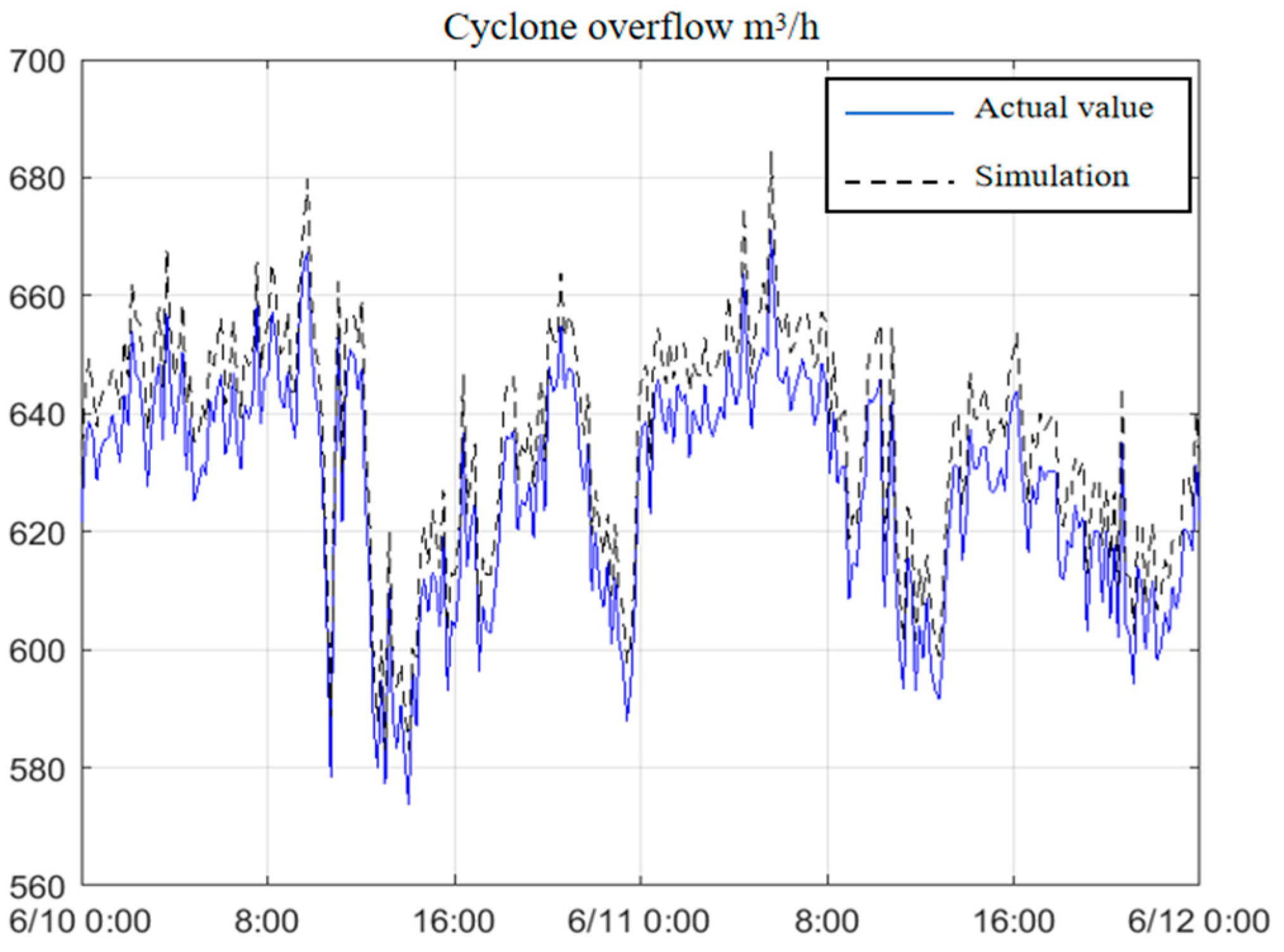
5.1.2. Cyclone Overflow Rate

Figure 6 shows the comparison between the measured flow rate of the cyclone and the simulation value. The blue curve represents the measured flow rate from a flowmeter, and the black curve represents the calculated value. After excluding abnormal data points, long-term comparison shows that the deviation between the simulated and measured values of the cyclone overflow flow rate is 1.62%.

Figure 6. Comparison between measured and simulated values of cyclone overflow.

5.1.3. Cyclone Overflow Concentration

Figure 7 shows the comparison between the measured and simulated values of the cyclone overflow concentration. The blue curve represents the measured value from the ray concentration meter, and the black curve represents the calculated value. After excluding abnormal data points, long-term comparison shows a mean square error of 3.40% between the simulation and measurement values for the cyclone overflow concentration.

Figure 7. Comparison between measured and simulated values. of cyclone overflow concentration.

5.2. Model Application

The crushing process is usually set before grinding. The big particles in raw ore will be crushed into smaller ones and then fed to the ball mills. The main function of offline simulation is to calculate the impact of changes in ball mill-feed particle size, which will happen at the start and stop of the crusher, and test the control rules for this situation. Figure 8 shows the variation trend in cyclone overflow particle size, which is all smaller than 74 microns, with no control operations. This can be regarded as the control group.

Figure 8. Cyclone overflow particle size (−74 microns) in control group.

When changing the feed rate into the ball mill under the same conditions in the control group, following the variation trend in Figure 9, the test group shows a narrow variation zone for cyclone overflow particle size distribution, which is better in application (Figure 9).

Figure 9. Ball mill feed rate in test group.

As shown in Figure 8, Figure 9 and Figure 10, when the ball milling-feed particle size changes before and after the crushing starts and stops, appropriate operation of the feed amount can effectively suppress the fluctuation of overflow particle size; moreover, when the feeding particle size becomes coarser, the simulation system can be used to test the operating range of the feeding amount to keep the overflow particle size within the target range.

Figure 10. Cyclone overflow particle size (−74 microns) in test group.

Based on the dynamic process model and the whole simulation system, the raw data from different sensors in the process can be cleaned and linked together for production analysis and even for making control rules. In this model application, the grinding product quality and the cyclone overflow particle size can be predicted on a virtual platform by the altering of operation movements. This is an easy, efficient, and accurate way to use the large amount of data in the mineral processing industry, and make profit, maintaining stable production in plants.

6. Conclusions

This paper utilizes prior knowledge to analyze multi-source signals containing time-varying factors that affect the grinding and classification process, and extracts their nonlinear feature vectors using the DBDAE method. On the basis of the universal mechanism model, a dynamic radial basis function network is used to learn the model’s errors and compensate, ultimately obtaining a multi-source compensation-driven grinding-classification process model. By designing and developing a simulation system for the grinding and classification process, the algorithm of the model is implemented. The industrial validation results indicate that the simulation results are consistent with the trends in measured values, and that the error can be maintained within a reasonable range. The method proposed in this article is feasible and has guiding significance for industry data application regarding the design of control methods for the mineral-processing grinding process.

References

1. Whiten, W.J. A matrix theory of comminution machines. Chem. Eng. Sci. 1974, 29, 589–599. [Google Scholar] [CrossRef]
2. Austin, L.; Barahona, C.; Weymont, N.; Suryanarayanan, K. An improved simulation model for semi-autogenous grinding. Powder Technol. 1986, 47, 265–283. [Google Scholar] [CrossRef]
3. Morrell, S.; Morrison, R.D. AG and SAG mill circuit selection and design by simulation. In Proceedings of the International Conference on Autogenous and Semiautogenous Grinding Technology, Vancouver, BC, Canada, 6–9 October 1996; Volume 2, pp. 769–790. [Google Scholar]
4. Nageswararao, K.; Wiseman, D.M.; Napier-Munn, T.J. Two empirical hydrocyclone models revisited. Miner. Eng. 2004, 17, 671–687. [Google Scholar] [CrossRef]
5. Bueno, M.P. Development of a Multi-Component Model Structure for Autogenous and Semi-Autogenous Mills. Ph. D Thesis, University of Queensland, Brisbane, Australia, 2013. [Google Scholar]
6. Song, T.; Yang, T.H.; Zhou, J.W.; Wang, Q. Process Modelling and Univariate Analysis of Comminution Circuits. IFAC-PapersOnLine 2018, 51, 19–23. [Google Scholar] [CrossRef]
7. De Oliveira, A.; de Carvalho, R.; Tavares, L. Predicting the effect of operating and design variables in grinding in a vertical stirred mill using a mechanistic mill model. Powder Technol. 2021, 387, 560–574. [Google Scholar] [CrossRef]
8. De Oliveira, A.; Tavares, L. Modeling and simulation of continuous open circuit dry grinding in a pilot-scale ball mill using Austin’s and Nomura’s models. Powder Technol. 2018, 340, 77–87. [Google Scholar] [CrossRef]
9. Srivastava, V.; Akdogan, G.; Ghosh, T.; Ganguli, R. Dynamic modeling and simulation of a SAG mill for mill charge characterization. Miner. Metall. Process. 2018, 35, 61–68. [Google Scholar] [CrossRef]
10. Zhang, Y.; Dai, Y.; Chen, L.; Xuan, B. Soft-measuring Model for Grinding Size Based on the Improved FOA-LSSVM Model. Min. Res. Dev. 2015, 35, 97–103. [Google Scholar]
11. Zhang, Y.; Chen, H.; Zhang, J. Soft-Measuring Model for Grinding Particle Size Based on the Improved GWO-LSSVM Model. Comput. Simul. China 2020, 37, 298–304. [Google Scholar]
12. Yu, P.; Xie, W.; Liu, L.X.; Powell, M.S. Analytical solution for the dynamic model of tumbling mills. Powder Technol. 2018, 337, 111–118. [Google Scholar] [CrossRef]
13. Li, H.; Evertsson, M.; Lindqvist, M.; Hulthén, E.; Asbjörnsson, G. Dynamic modeling and simulation of a SAG mill-pebble crusher circuit by controlling crusher operational parameters. Miner. Eng. 2018, 127, 98–104. [Google Scholar] [CrossRef]
14. Yuwen, C.; Sun, B.; Liu, S. A Dynamic Model for a Class of Semi-Autogenous Mill Systems. IEEE Access 2020, 8, 98460–98470. [Google Scholar] [CrossRef]
15. Liu, Y.; Spencer, S. Dynamic simulation of grinding circuits. Miner. Eng. 2004, 17, 1189–1198. [Google Scholar] [CrossRef]
16. Wang, Z. Dynamic Simulation of Grinding and Classification Process and Its Application; Tsinghua University: Beijing, China, 2014. [Google Scholar]
17. Légaré, B.; Bouchard, J.; Poulin, É. A modular dynamic simulation model for comminution circuits. IFAC-PapersOnLine 2016, 49, 19–24. [Google Scholar] [CrossRef]
18. Nageswararao, K. Further Developments in the Modelling Scale-Up of Industrial Hydrocyclones. Ph.D. Thesis, University of Queensland (JKMRC), Brisbane, Australia, 1978. [Google Scholar]
19. Langarica, S.; Pizarro, G.; Poblete, P.; Radrigan, F.; Pereda, J.; Rodriguez, J.; Nunez, F. Denoising and Voltage Estimation in Modular Multilevel Converters Using Deep Neural-Networks. IEEE Access 2020, 8, 207973–207981. [Google Scholar] [CrossRef]
20. Qiao, J.; Han, H. Optimal structure design for RBFNN structure. Acta Auto-Mica Sin. 2010, 36, 865–872. [Google Scholar] [CrossRef]
21. Xie, C.; Ma, H.; Song, T.; Zhao, Y. DEM investigation of SAG mill with spherical grinding media and non-spherical ore based on polyhedron-sphere contact model. Powder Technol. 2021, 386, 154–165. [Google Scholar] [CrossRef]
22. Hasankhoei, A.R.; Maleki-Moghaddam, M.; Haji-Zadeh, A.; Barzgar, M.E.; Banisi, S. On dry SAG mills end liners: Physical modeling, DEM-based characterization and industrial outcomes of a new design. Miner. Eng. 2019, 141, 105835. [Google Scholar] [CrossRef]
23. Owusu, K.B.; Zanin, M.; Skinner, W.; Asamoah, R.K. AG/SAG mill acoustic emissions characterisation under different operating conditions. Miner. Eng. 2021, 171, 107098. [Google Scholar] [CrossRef]
Disclaimer/Publisher’s Note: The statements, opinions and data contained in all publications are solely those of the individual author(s) and contributor(s) and not of MDPI and/or the editor(s). MDPI and/or the editor(s) disclaim responsibility for any injury to people or property resulting from any ideas, methods, instructions or products referred to in the content.
Article Metrics
Citations
Article Access Statistics
Multiple requests from the same IP address are counted as one view.