Abstract
The transient electromagnetic method (TEM) is widely used in the exploration of mineral, petroleum, and geothermal resources due to its sensitivity to low-resistivity bodies, limited site constraints, and strong resistance to interference. In practical applications, the TEM often uses a long wire source instead of an idealized horizontal electric dipole (HED) source as the excitation source. This is due to the complex external conditions and the relatively large distance between the receiving zone and the transmitter source. Compared to the HED, the long wire source can provide a larger excitation current, generating stronger signals to meet the requirements of a higher signal-to-noise ratio or deeper exploration. It also produces longer-duration signals, thereby providing better resolution. Additionally, for the interpretation of TEM data, three-dimensional forward modeling plays a crucial role. However, the mature traditional TEM forward method is based on a simple, sometimes inappropriate model, as it is well established that the induced polarization (IP) effect is widely present in the deep earth, especially in oil and gas reservoirs. The presence of the IP effect results in negative responses in field data that do not conform to the traditional theoretical decay law of TEM, which can significantly impact data processing and inversion results. To address this issue, a TEM forward modeling method considering the IP effect based on the spectral element method (SEM) has been developed in this study. Firstly, starting from the Helmholtz equation satisfied by the time domain electric field, we introduce the Debye model with polarization information into the forward modeling by utilizing the differential form of Ohm’s law. As a result, we derive the boundary value problem for the time domain electric field that considers the induced polarization effect. Using Gauss–Lobatto–Legendre (GLL) polynomials as the basis functions, the SEM is employed to discretize the governing equations at each time step and obtain spectral element discretization equations. Then, temporal discretization equations are derived using the second-order backward Euler formula, and the linear system of equations is solved using the Pardiso direct solver. Finally, the electromagnetic responses at any time channel are obtained via SEM interpolation and numerical integration, thereby achieving three-dimensional TEM forward modeling considering the IP effect. The results indicate that this method can effectively reflect the spatial distribution of polarizable subsurface media. It provides valuable references for studying the polarization parameters of subsurface media and performing a three-dimensional inversion of TEM data considering the induced polarization effect.
1. Introduction
The transient electromagnetic method (TEM) is a time-domain electromagnetic exploration method that uses a step wave or pulse current as an excitation source to measure the pure secondary field after the primary field is turned off [1,2]. Due to the broadband nature of the emitted waveforms, which have high resolution, greater detection depth, sensitivity to good conductors, and less susceptibility to terrain limitations, TEM is widely applied in practical fields such as mineral resource exploration [3]. For example, Strack conducted test surveys using the loop-source transient electromagnetic method in the Sydney Basin. The inverted geoelectric results showed a qualitative correspondence with the local geological conditions, indicating the feasibility of the transient electromagnetic method in deep mineral and oil/gas exploration [4]. Yan et al. utilized the long-offset transient electromagnetic method to identify local structures in the southern carbonate rock region [5]. Cheng et al. employed the transient electromagnetic method to predict the water-rich level of rock layers near boreholes, which is crucial for safe mineral production [6]. Yang et al. utilized the transient electromagnetic method for hydrogeological exploration in the Longdong coal mining area to determine the extent of abnormal areas in goaf regions [7]. TEM relies on inversion to reconstruct underground models, and inversion accuracy is based on selecting an appropriate forward modeling method. Traditional transient electromagnetic forward modeling methods include the Integral Equation Method (IEM) [8,9,10], Finite Difference Method (FDM) [11,12,13,14], Finite Element Method (FEM) [15,16,17,18], Finite Volume Method (FVM) [19,20,21], and Spectral Element Method (SEM) [22,23,24]. Among them, the IEM only requires the physical grid discretization of the anomalous body region rather than the entire computational domain. This effectively reduces the number of unknowns, resulting in a smaller system of linear equations and faster computation speed, thus achieving higher solving efficiency. However, the resulting coefficient matrix of the IEM is dense and asymmetric. When simulating complex geoelectric models, the grid partitioning needs to be fine enough to meet the computational accuracy requirements, leading to large memory requirements and inflexibility in simulating complex models. The FDM discretizes the computational domain with regular hexahedral grids and places degrees of freedom at nodes, edges, and faces, making it intuitive and easy to implement in programming. However, due to the limitations of grid partitioning formats, the computational accuracy is affected, especially in the simulation of complex models, where severe trapezoidal or stepped approximations may occur. The FEM can discretize the computational domain using regular hexahedra or unstructured tetrahedra, providing more flexibility in simulating complex models. However, the detailed grid partitioning leads to a more complex coefficient matrix, limiting computational efficiency. The FVM is considered to be a numerical simulation method derived from both finite element and finite difference methods, combining their advantages and disadvantages. The SEM used in this study is a numerical simulation method that combines the ideas of finite element and spectral methods. It performs high-order spectral integration operations within each finite element discretized grid. SEM provides flexibility in simulating complex geoelectric models and inherits the exponential convergence properties of spectral methods, achieving optimal computational efficiency while ensuring computational accuracy [25].
In recent years, TEM forward modeling techniques have gradually matured due to updates in forward modeling methods and the optimization of computational efficiency [26,27,28]. When conducting forward simulations for mineral exploration, it is typically assumed that the electrical resistivity of the subsurface medium is a real-valued quantity. However, studies have shown that rock formations such as shale, which contains small pores and fractures, exhibit significant polarization effects [29,30]. With the increasing demand for unconventional oil and gas exploration, such as shale gas, the traditional methods that only consider real-valued electrical resistivity are unable to effectively explain the negative response phenomena observed in collected data, which leads to deviations between the inversion results and the actual geological conditions. Therefore, the development of three-dimensional TEM forward modeling considering the induced polarization (IP) phenomenon caused by the frequency dispersion of rock conductivity in the electromagnetic exploration frequency range is urgently needed [31,32]. Man et al. calculated the time domain electromagnetic field response considering the IP effects using a frequency–time conversion method in finite difference forward modeling [33]. To overcome the limitations of the frequency–time conversion method, Zhang et al. directly introduced a complex resistivity model into the time domain governing the equations of unstructured finite element modeling and performed airborne transient electromagnetic three-dimensional forward modeling [34]. However, in TEM forward modeling that considers the IP effect, the commonly used electromagnetic field excitation sources are mainly loop sources, and there is limited research on long wire sources, which poses more challenges [35,36]. Compared to loop source transient electromagnetic, the long wire source method provides higher resolution, is suitable for deep exploration, and better meets the current demands for unconventional oil and gas resource exploration [37,38]. Furthermore, there are various models available to describe the frequency dispersion characteristics of polarizable rock formations, such as the Debye model [39], Cole–Cole model [40], Wait model [41], Dias model [42], GEMTIP model [43,44], and Zonge model [45,46]. Among these models, the Debye model has a wide range of applications. It can simulate the frequency dispersion characteristics of solid, liquid, and mixed-phase media conductivity. It is suitable for simulating complex underground media with multiple phases and porosity. The Debye model is relatively simple, with fewer induced polarization parameters, making it easier to implement in numerical simulations.
This study conducted three-dimensional TEM forward modeling simulations using the long wire source and considering the IP effect based on the Debye model. Firstly, the accuracy and effectiveness of the algorithm were verified by comparing the results with the one-dimensional solutions for a homogeneous half-space and layered media. Then, the influence of different IP parameters on the electric field response curves was analyzed, followed by the simulation of the three-dimensional electric field response of underground low-resistivity polarizable bodies and multiple regular anomalous bodies. Finally, by combining the model based on the real physical parameters of a shale gas field, the three-dimensional transient electromagnetic response characteristics during multi-stage hydraulic fracturing were studied, demonstrating the effectiveness and feasibility of the three-dimensional transient electromagnetic spectral element method considering the induced polarization effect in monitoring multi-stage hydraulic fracturing.
2. Spectral Element Method
2.1. Boundary Value Problems and Variational Problems
In TEM forward modeling based on the SEM, conduction current predominates, so the displacement current term is typically neglected. In this case, the diffusion equation for the electric field is satisfied:
where E represents the electric field intensity, μ is the magnetic permeability, Je is the conduction current density, and Js is the source current density. The source term in this article is a long wire source, which can be considered as the cumulative effect of the electric field generated by countless tiny electric dipoles.
To ensure the uniqueness of the solution for the time domain electromagnetic field, boundary conditions need to be applied within the computational domain and on its boundaries. Additionally, initial conditions need to be imposed on the field values. The tangential electric field continuity must be satisfied at the interfaces between different media within the computational domain:
where E1 and E2 represent the electric fields on the two sides of the interface between two different media. At the boundaries, it is assumed that the electromagnetic field attenuates with increasing distance from the source at the boundaries. When the physical extent of the domain is large enough, the electric field at the boundaries is 0, thus requiring Dirichlet boundary conditions:
The initial conditions for time-domain transient electromagnetic problems can be complex and depend on the type and waveform of the excitation source. In this paper, considering a long wire electric source as the excitation source, when the transmitted waveform is a downward step wave, the initial conditions are as follows:
where EDC represents a steady-state electric field generated via a direct current (DC) flow. When the excitation waveform is any other arbitrary waveform, the initial conditions are as follows:
To simplify the solution process, it is necessary to transform the boundary value problem in its differential form into an integral form using the Galerkin weighted residual method. This leads to a weak formulation problem that can be solved. The residual form of the time-domain governing equation is defined as follows:
In this paper, the SEM is employed to discretize the computational domain into multiple elements (Figure 1). The residual of the nth element Ωe is defined as . By applying the Galerkin weighted residual method and performing the necessary manipulations, the following expression is obtained:
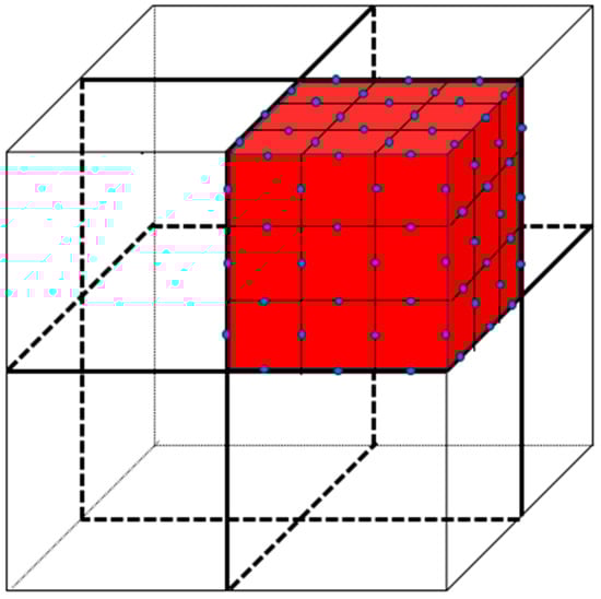
Figure 1.
Spectral element discretization diagram (where the red region represents a single discretized element, and the blue dots represent the placement of basis functions within the element).
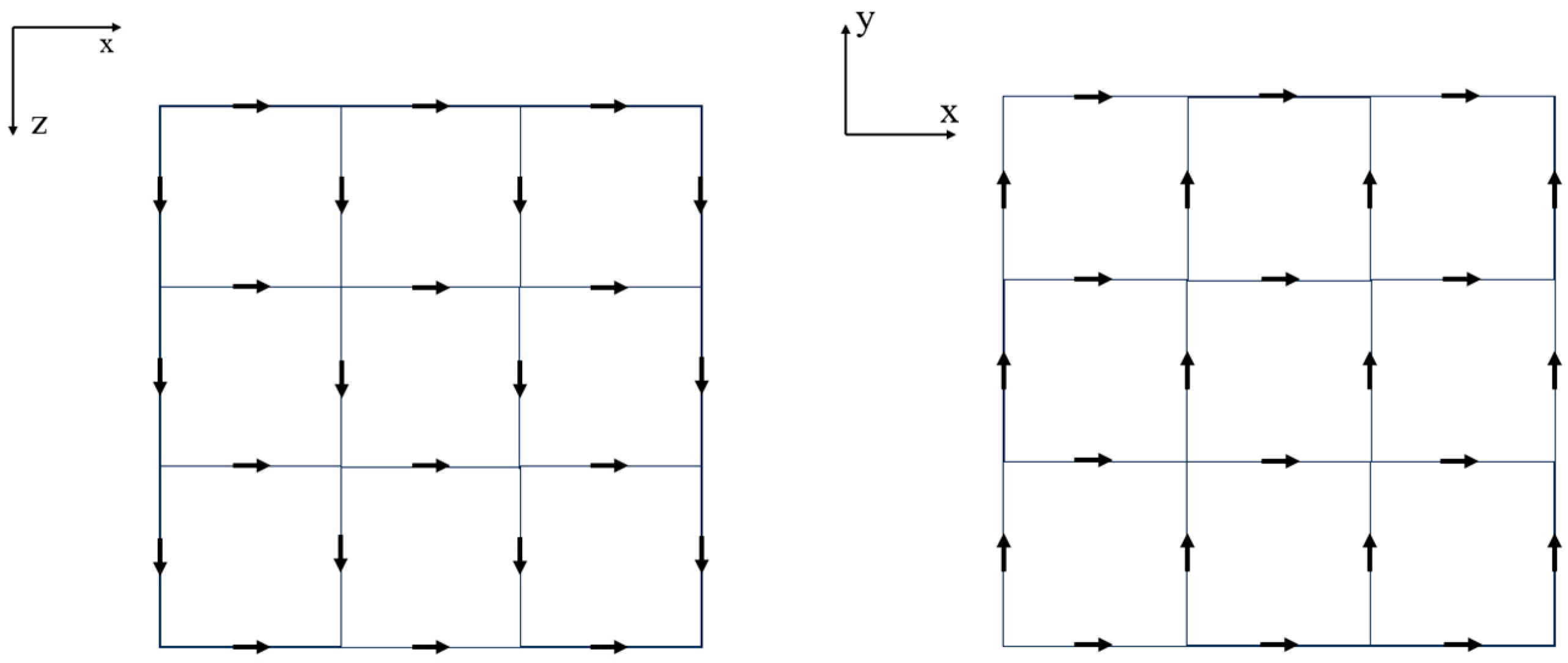
Here, ν represents the weight function. When using the spectral element method for solving, the weight function is chosen as the three-dimensional vector high-order spectral element basis function formed via Gauss–Lobatto–Legendre (GLL) polynomials. Similar to the FEM, the scalar SEM cannot satisfy the physical boundary conditions of vector electromagnetic fields, leading to spurious solutions in the computed results. On the other hand, the vector SEM can automatically satisfy the internal boundary conditions of the governing equations. Therefore, this paper adopts the vector spectral element method to solve the transient electromagnetic forward problem. The placement of degrees of freedom within the interior plane of the element is shown in the figure (Figure 2).
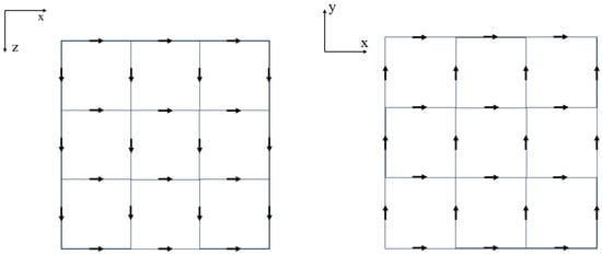
Figure 2.
Schematic diagram of the placement of degrees of freedom in each direction within the interior plane of the element.
2.2. SEM Considering the IP Effect
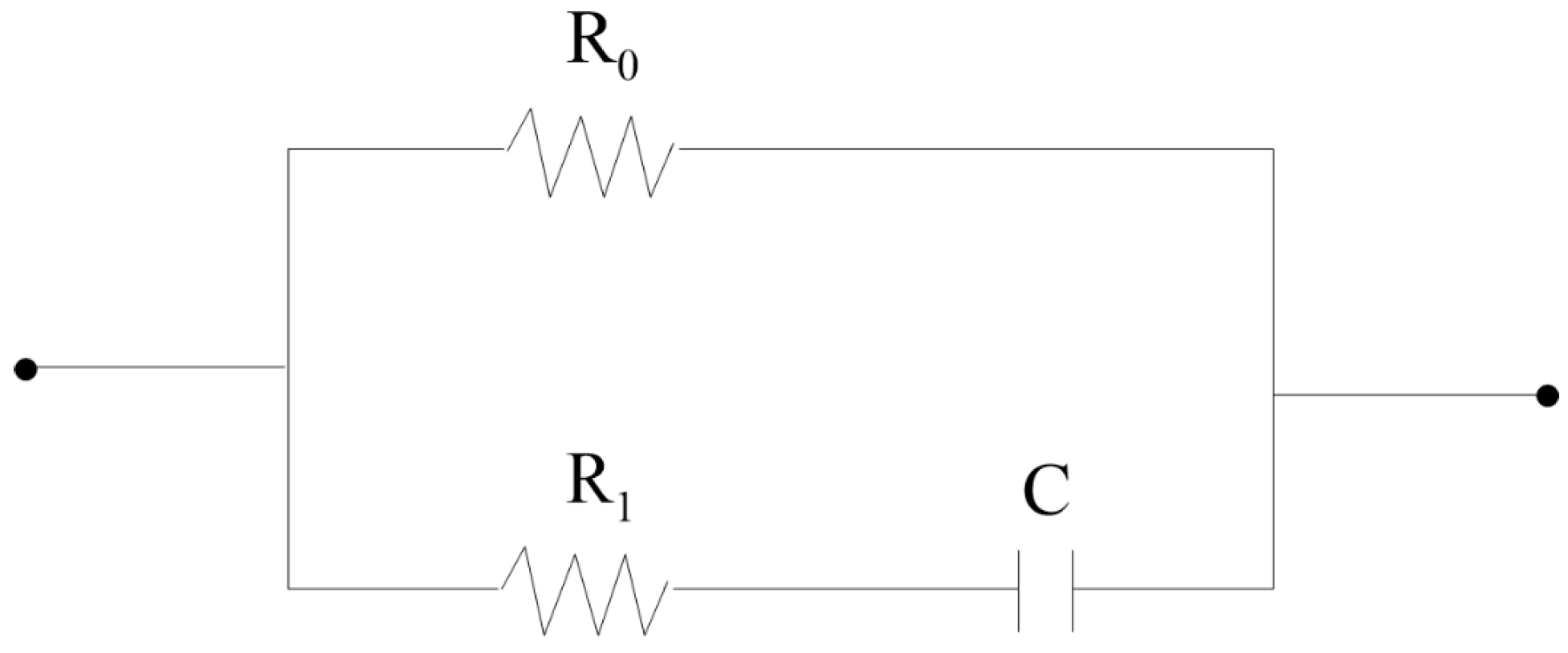
Considering the frequency dispersion of conductivity in forward simulations can effectively control the issue of non-uniqueness in inversion. In this paper, the Debye model (Figure 3) is introduced into the transient electromagnetic spectral element method.

Figure 3.
Equivalent circuit diagram of the Debye model.
The conduction current density Je in the conventional control equation can be described using the differential form of Ohm’s law, which is
In the above equation, σ represents the conductivity. The conductivity exhibits frequency dispersion when the subsurface anomaly is a polarizable medium. It can be described using the Debye model as follows:
In the above equation, σ0 represents the zero-frequency resistivity, m represents the polarizability, ω represents the angular frequency, τ represents the time constant, and i represents the imaginary unit. In the frequency domain, by substituting Equation (9) into Equation (8) and rearranging them, we obtain
By performing the inverse Fourier transform, we can convert it from the frequency domain to the time domain:
To ensure a stable discretization in the time domain and accurate forward simulation results, this paper adopts a variable step-size second-order backward Euler approximation formula:
where Ft represents the field value at time t, Δt represents the time step size, and Kn represents the ratio of adjacent time steps. After discretizing in the time domain, we can derive the formula for calculating the time domain conduction current density. Substituting it into the conventional time domain control equation (Equation (1)) and rearranging them, we obtain the time domain spectral element control equation considering the IP effect:
where
3. Accuracy Verification
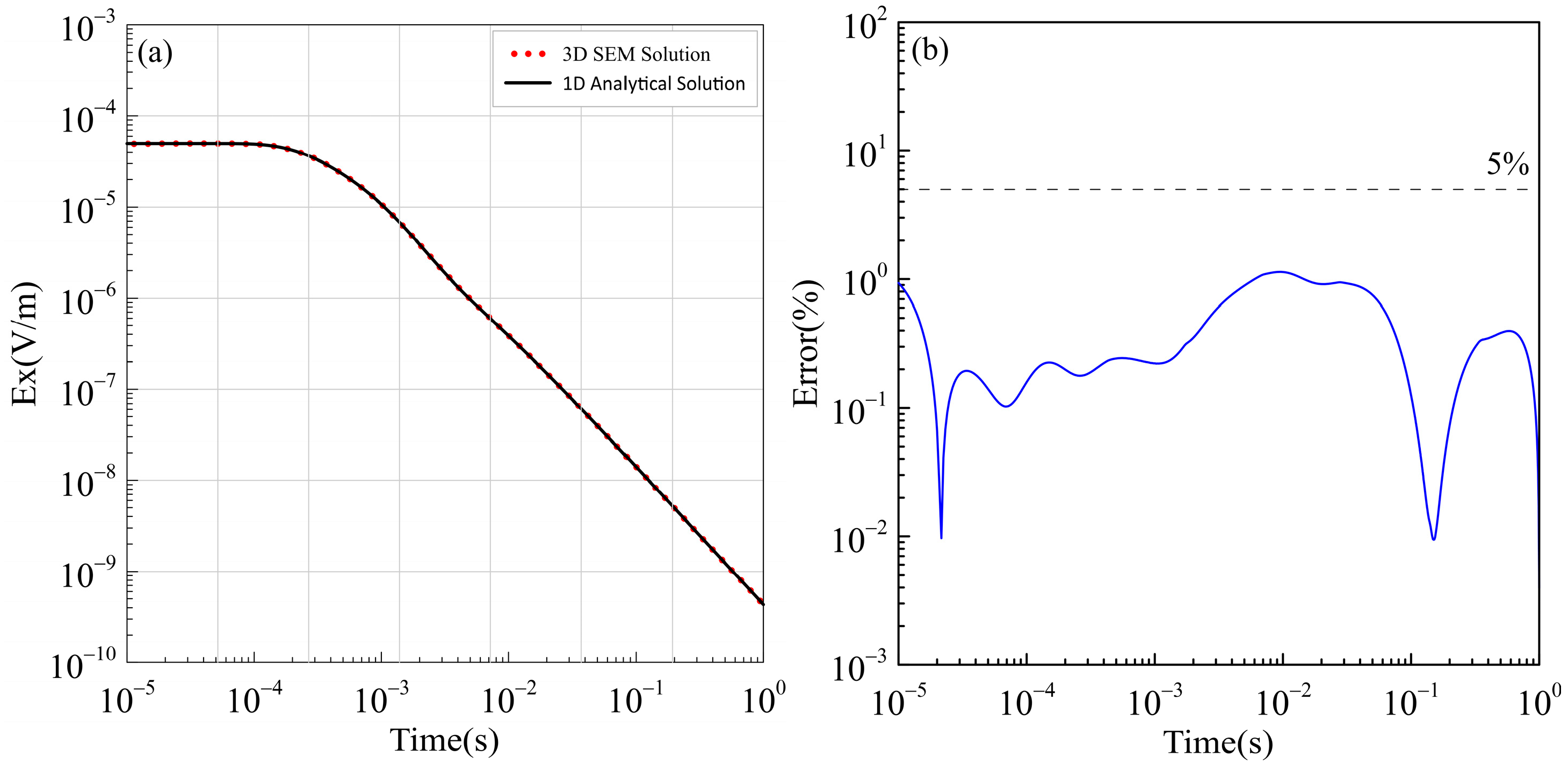
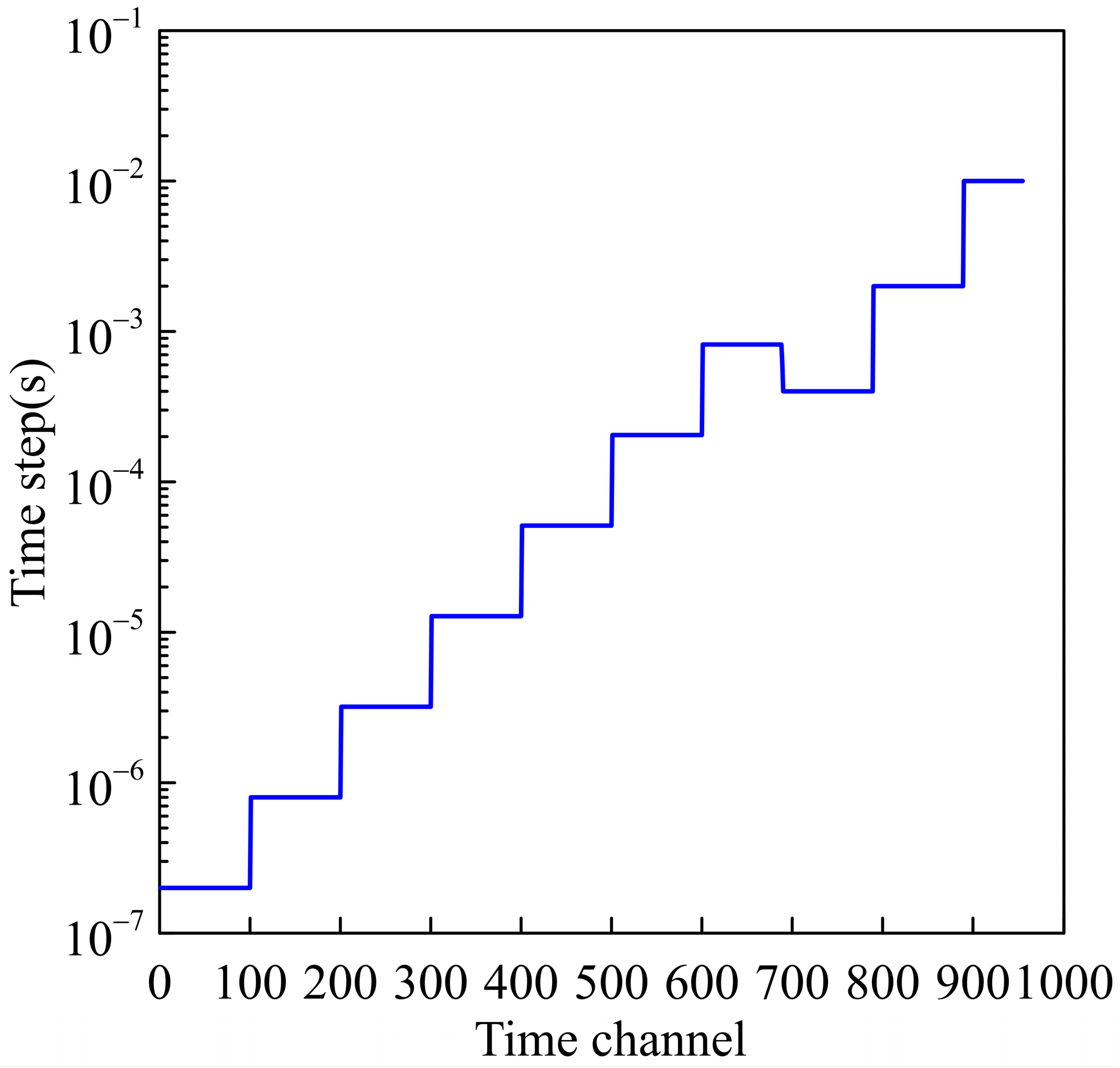
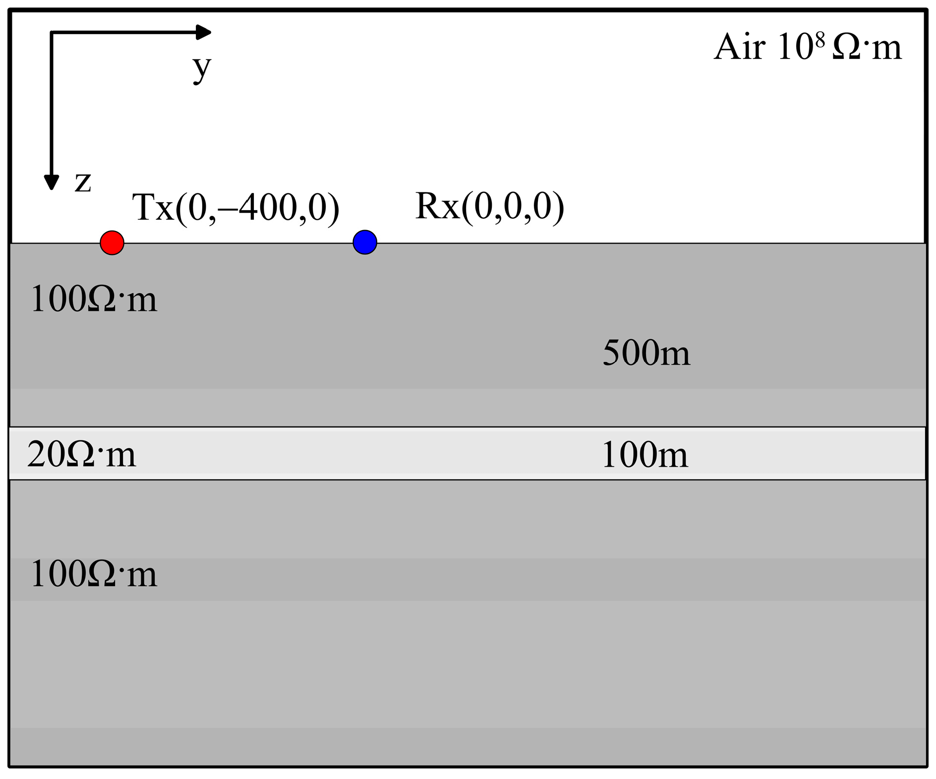
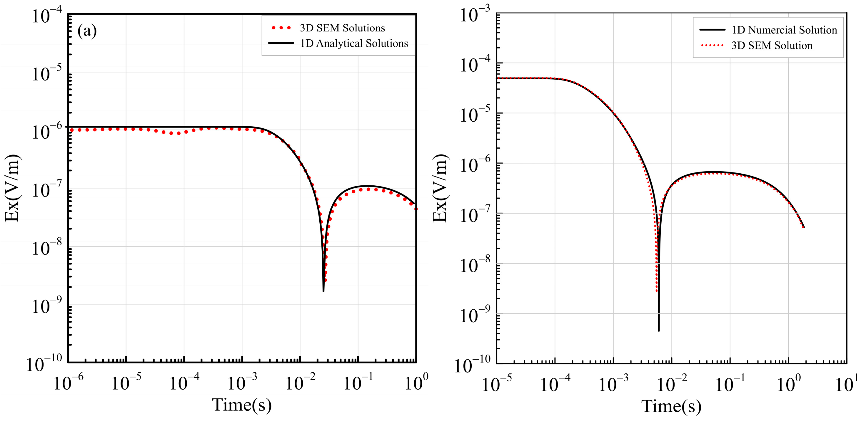
To ensure the accuracy of the algorithm, this study utilized the proposed method to calculate the electric field response in a layered medium and compared it with the one-dimensional analytical solution with the same parameters (Figure 4a). The stratigraphic parameters are set as follows: the thicknesses are 500 m, 100 m, and infinite, and the resistivities are 100 Ω·m, 20 Ω·m, and 100 Ω·m, respectively. Figure 4b shows the relative error between the two methods. In terms of algorithm parameters, the spectral element method was set to order 3, resulting in a total of 6480 elements, 184,525 nodes, and 543,840 degrees of freedom after mesh refinement, the time steps are shown in Figure 5. Each time step calculation requires two calls to the Pardiso solver to solve a linear system of equations. In the initial call, assigning the right-hand side takes about 15 s, followed by an LU decomposition step that takes around 11 s. Then, a back substitution step takes about 0.15 s. Subsequently, only back substitution is performed until a change in the time step occurs, at which point the right-hand side changes, and the above operations need to be repeated. From the figure, it can be observed that the relative error between the two methods is below 5%, meeting the required accuracy and demonstrating the practical feasibility of the algorithm. Additionally, this study considered a homogeneous half-space model with a source length of 1000 m, offset distance of 5000 m, subsurface resistivity of 1000 Ω·m, polarization rate of 0.1, and time constant of 1. A three-layer dielectric model with a low-resistivity polarization layer in the intermediate layer, as shown in Table 1, was also investigated (Figure 6). The electric field responses were obtained using both the spectral element method and the one-dimensional numerical simulation (Figure 7a,b). From Figure 7, it can be observed that under the same observation parameters, the electric field response obtained using the proposed algorithm exhibits a high degree of agreement with the corresponding one-dimensional numerical simulation curve [47].
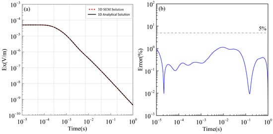
Figure 4.
Validation of transient electromagnetic spectral element method in a three-layered medium: (a) Comparison of the electric field response between spectral element method and one-dimensional analytical solution; (b) Relative error plot.
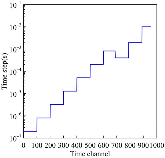
Figure 5.
Diagram of time step.

Table 1.
Parameters of the three-layered medium model considering the IP effect.

Figure 6.
Schematic diagram of the three-layered medium model.
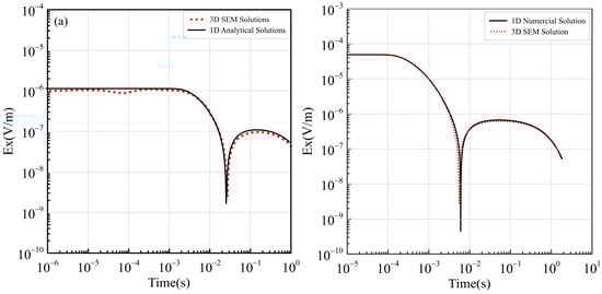
Figure 7.
Comparison of electric field responses between the spectral element method considering the IP effect and the one-dimensional numerical simulation for (a) a homogeneous half-space and (b) a layered model.
4. Numerical Experiments
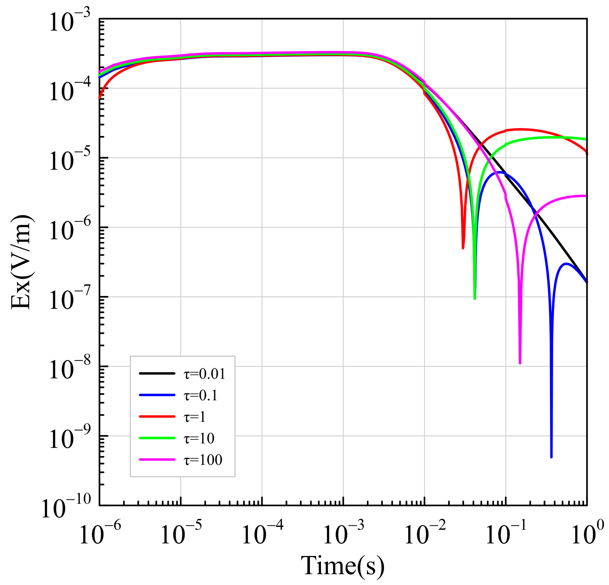
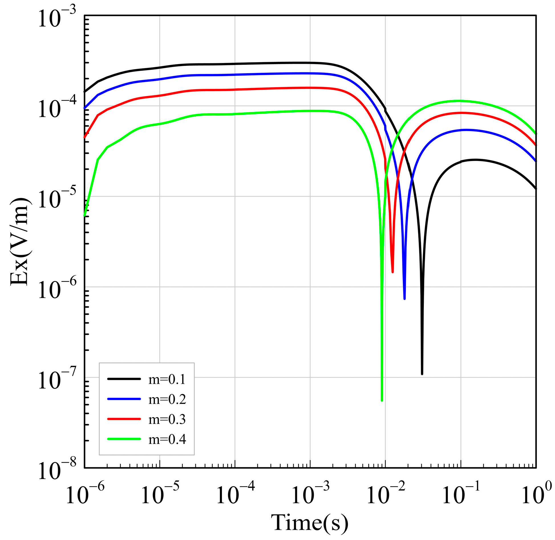
To investigate the influence of different IP parameters of subsurface media on the electric field response curves for the accurate inversion of subsurface structures and rock properties, a homogeneous polarizable half-space model with a resistivity of 1000 Ω·m is set up. The polarization factor, denoted as “m”, is controlled at 0.1. The variable time constant τ is changed to 0.01 ms, 0.1 ms, 1 ms, 10 ms, and 100 ms, respectively. The electric field responses are calculated and plotted for comparison to observe the effect of different time constants on the electric field response. From Figure 8, it can be observed that when the time constant is less than 1 s, the smaller the value of τ, the later the negative response of the electric field appears and the smaller its amplitude. When the time constant is greater than 1 s, the smaller the value of τ, the earlier the negative response of the electric field appears and the larger its amplitude. Furthermore, with the time constant τ set to 0.1 s, the polarization factor “m” is changed to 0.1, 0.2, 0.3, and 0.4, respectively. The corresponding electric field responses are calculated and plotted for comparison to observe the effect of different polarization factors on the electric field response. Figure 9 shows that as the polarization factor increases, the negative response of the electric field appears earlier and with a larger amplitude.

Figure 8.
Electric field responses with different time constants in a homogeneous half-space.
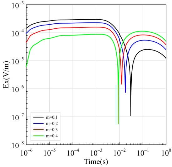
Figure 9.
Electric field responses with different polarizabilities in a homogeneous half-space.
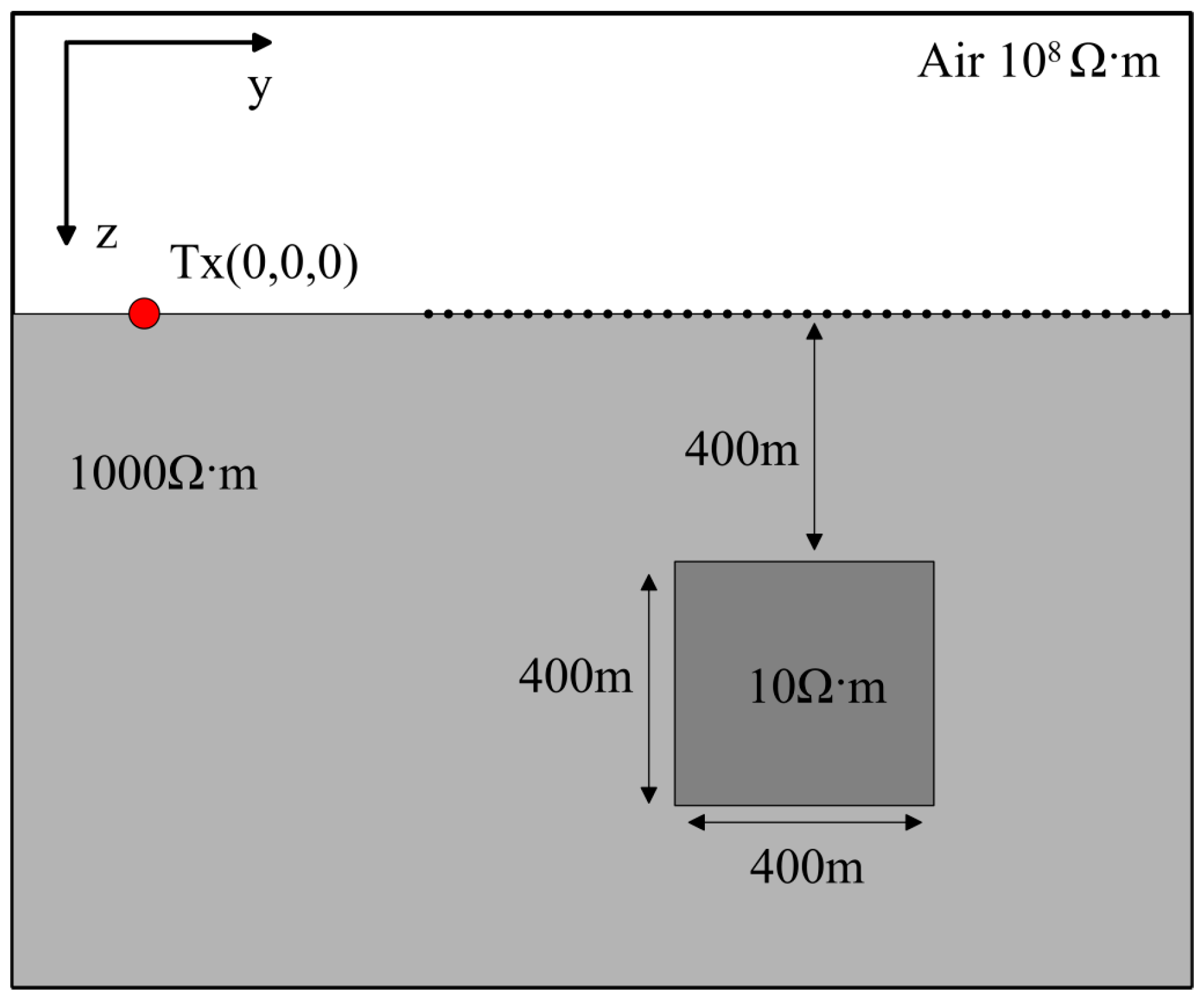
In addition, this study designed underground models of a low-resistivity anomaly and multiple anomalies to investigate the electric field response characteristics of polarized underground bodies. Figure 10 shows the model of the low-resistivity anomaly, with a 600 m long wire source as the transmitter, a current intensity of 100 A, a measurement grid of 600 m × 800 m, a spacing of 50 m between measurement points, a total of 221 measurement points, and an anomaly size of 200 m × 400 m × 400 m. The resistivity of the anomaly is 10 Ω·m, the polarizability is 0.5, the time constant is 1 s, and it is buried at a depth of 400 m. The resistivity of the surrounding rock is 1000 Ω·m.
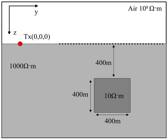
Figure 10.
Model of a low-resistivity polarized anomaly.
Figure 11 illustrates the electric field responses of a polarized anomaly with low resistivity at various time channels in the xy plane. Figure 11a–e correspond to the responses at time channels of 0.01 ms, 0.1 ms, 1 ms, 10 ms, and 55 ms, respectively. The white dashed line represents the position of the anomaly. The electric field response values gradually decay over time. In the early stage, the electric field response to the anomaly decays faster compared to the surrounding rock, while in the later stage, the decay is slower, and the response values are higher than the surrounding rock. By analyzing the decay of the electric field response over time, we can make an approximate inference about the distribution of the anomaly body in the xy plane.
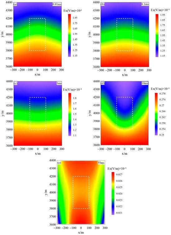
Figure 11.
Electric field response at different time gates in the xy plane for a low-resistivity polarized anomaly (The white dashed box indicates the location of the anomaly): (a) 0.01 ms, (b) 0.1 ms, (c) 1 ms, (d) 10 ms, and (e) 55 ms.
Figure 12 shows the computed electric field responses in the xz plane for the low-resistivity polarized anomaly model from Figure 10. Figure 12a–e correspond to the electric field responses at time channels of 0.01 ms, 0.1 ms, 1 ms, 10 ms, and 100 ms, respectively. The white dashed line represents the position of the anomaly. From the figure, it can be observed that at the initial time channel, the region of the anomaly displays a higher electric field value compared to the surrounding rock. As time progresses, the electric field gradually starts to decay. At 1 ms, the anomaly region displays a lower electric field response compared to the surrounding rock. At 10 ms, the anomaly region is accurately displayed, and at 100 ms, negative response values appear in the anomaly region. Additionally, from the figure, the buried depth and size of the low-resistivity polarized anomaly can be inferred.
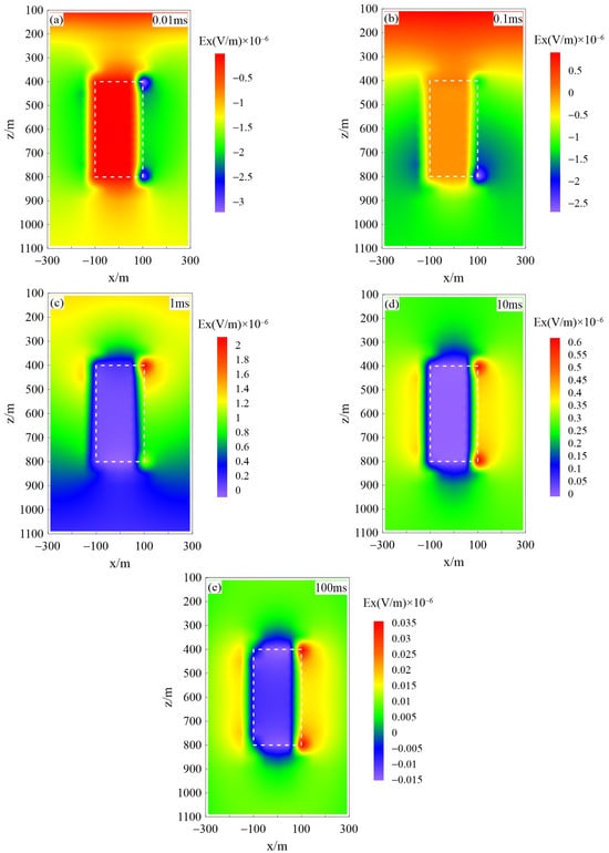
Figure 12.
Electric field response at different time channels in the xy plane for a low-resistivity polarized anomaly (The white dashed box indicates the location of the anomaly): (a) 0.01 ms, (b) 0.1 ms, (c) 1 ms, (d) 10 ms, and (e) 55 ms.
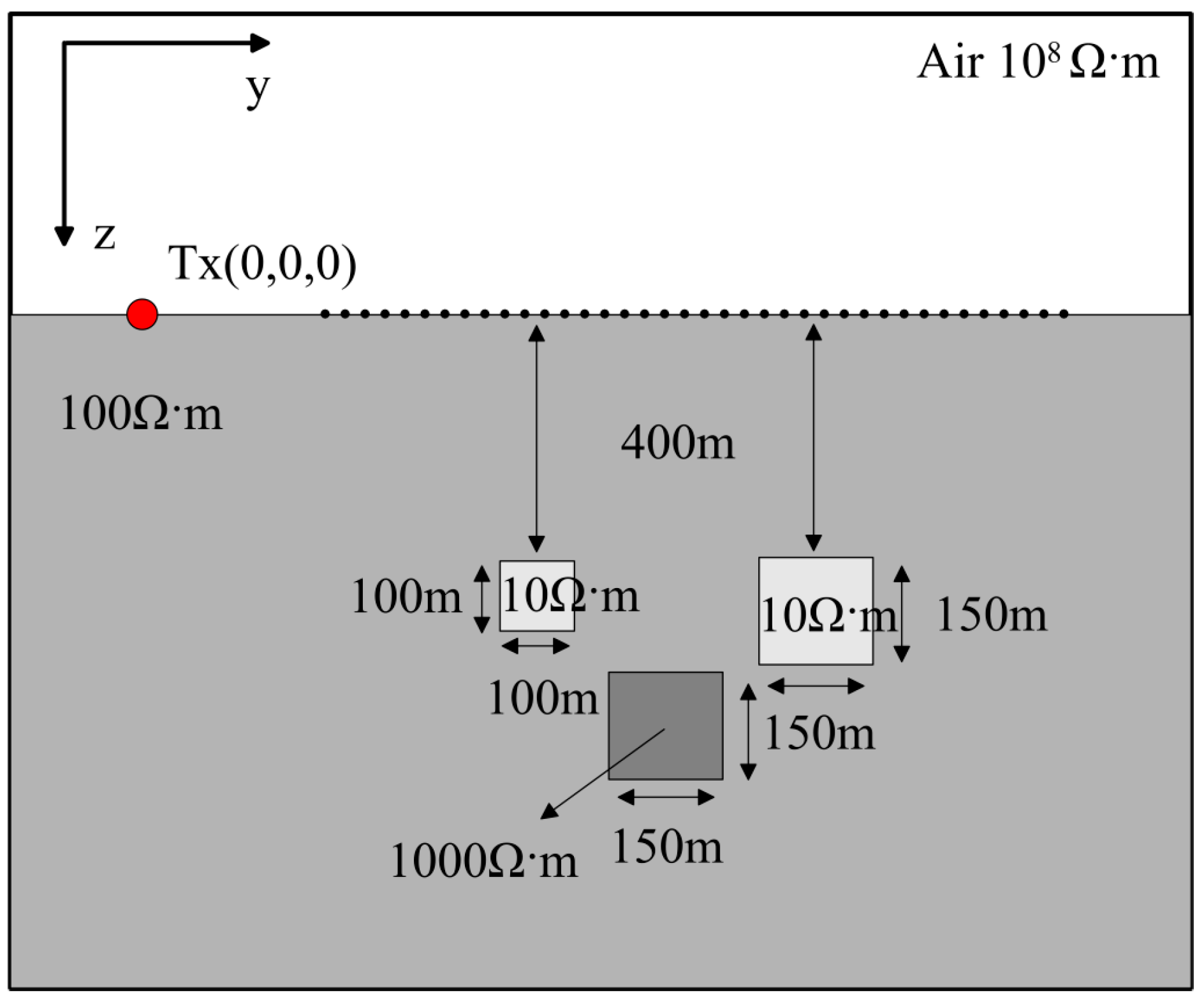
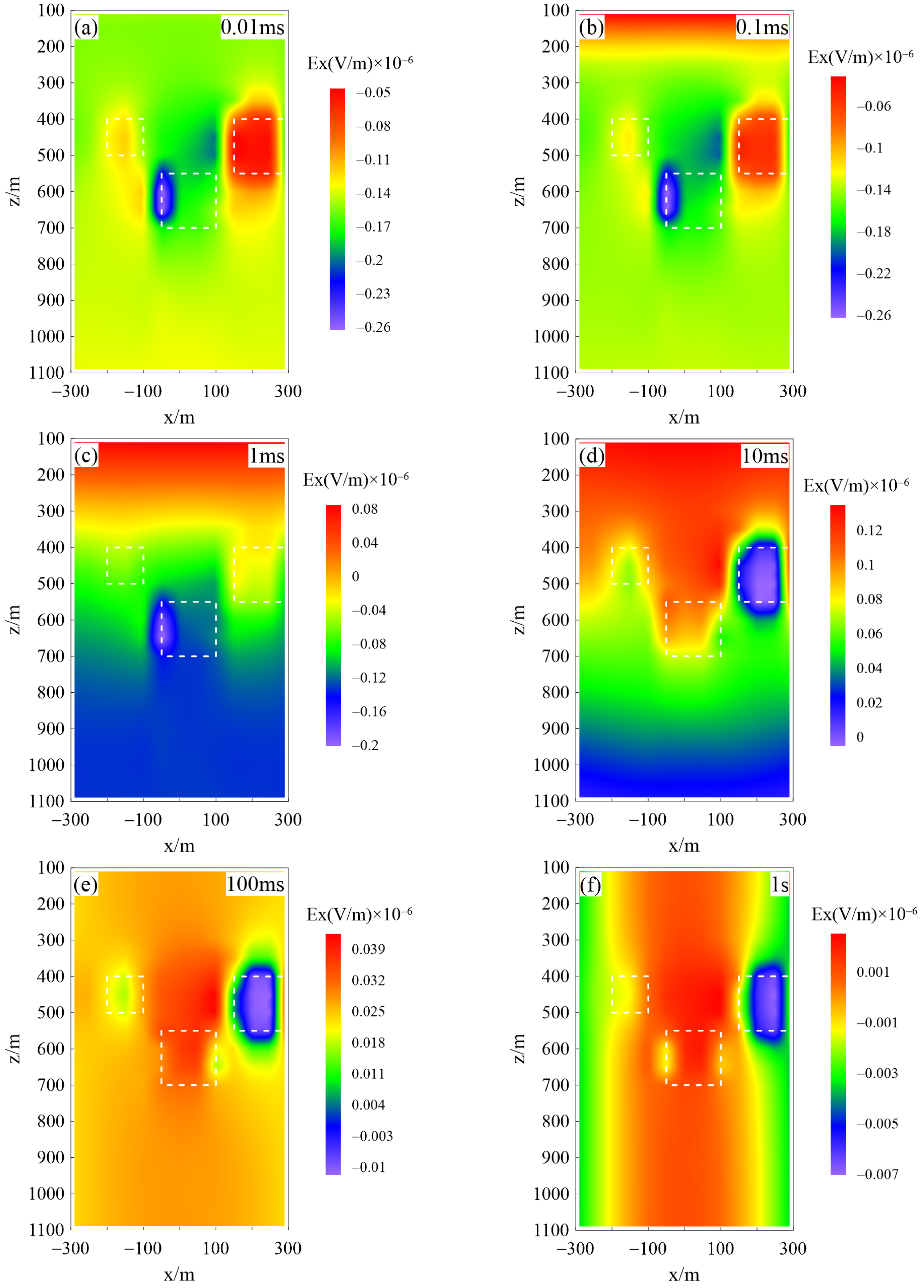
To explore the application prospects of the TEM considering the IP effect based on the SEM in complex underground media, multiple models of relatively low-resistivity or high-resistivity anomalies were designed (Figure 13). The transmitter length was 600 m, and the burial depths of the anomalies were 400 m, 550 m, and 400 m, respectively. The sizes of the anomalies were 100 m × 100 m × 100 m, 150 m × 150 m × 150 m, and 150 m × 100 m×150 m, with resistivities of 10 Ω·m, 1000 Ω·m, and 10 Ω·m, respectively. The surrounding rock had a resistivity of 100 Ω·m., and the polarizability of the anomalies was 0.5, with a time constant of 1. Figure 14 illustrates the electric field responses of multiple polarized anomalies in the xz plane. The white dashed lines indicate the positions of the anomalies. It can be observed from the figure that this method can simultaneously reflect the approximate positions of multiple polarized anomalies underground. However, it exhibits higher sensitivity towards low-resistivity anomalies, and the response to these anomalies is more pronounced at 10 ms. Compared to low-resistivity polarized bodies, high-resistivity polarized bodies exhibit more intense negative responses with larger amplitudes.
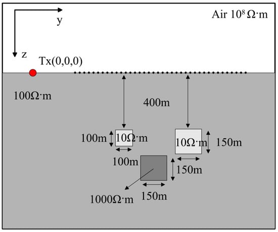
Figure 13.
Multiple models of polarized anomaly bodies in the subsurface.

Figure 14.
Electric field response at different channels in the xz plane for multiple polarized anomaly bodies (The white dashed box indicates the location of the anomaly): (a) 0.01 ms, (b) 0.1 ms, (c) 1 ms, (d) 10 ms, (e) 100 ms, and (f) 1 s.
5. Three-Dimensional Forward Modeling of Hydraulic Fracturing
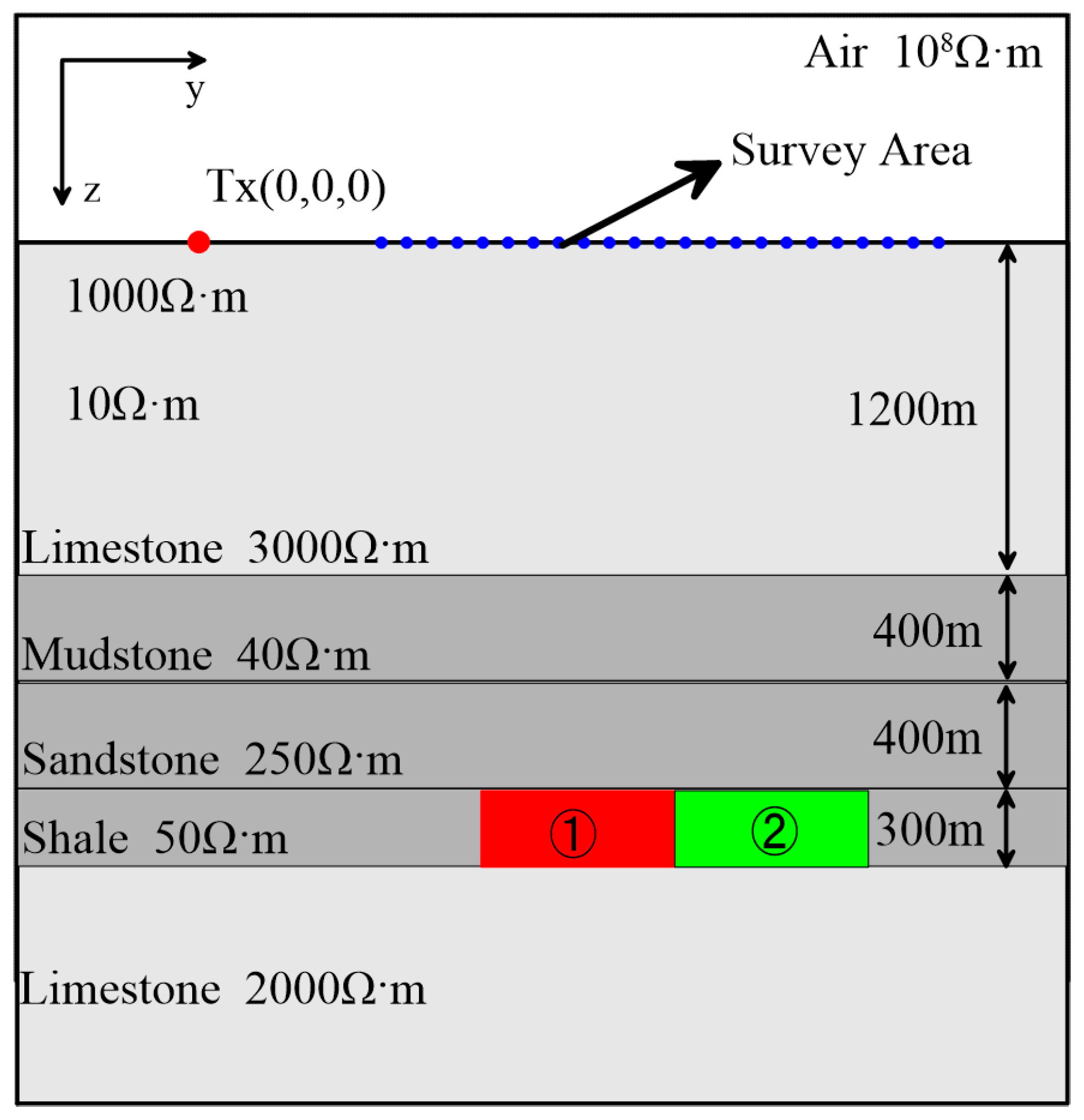
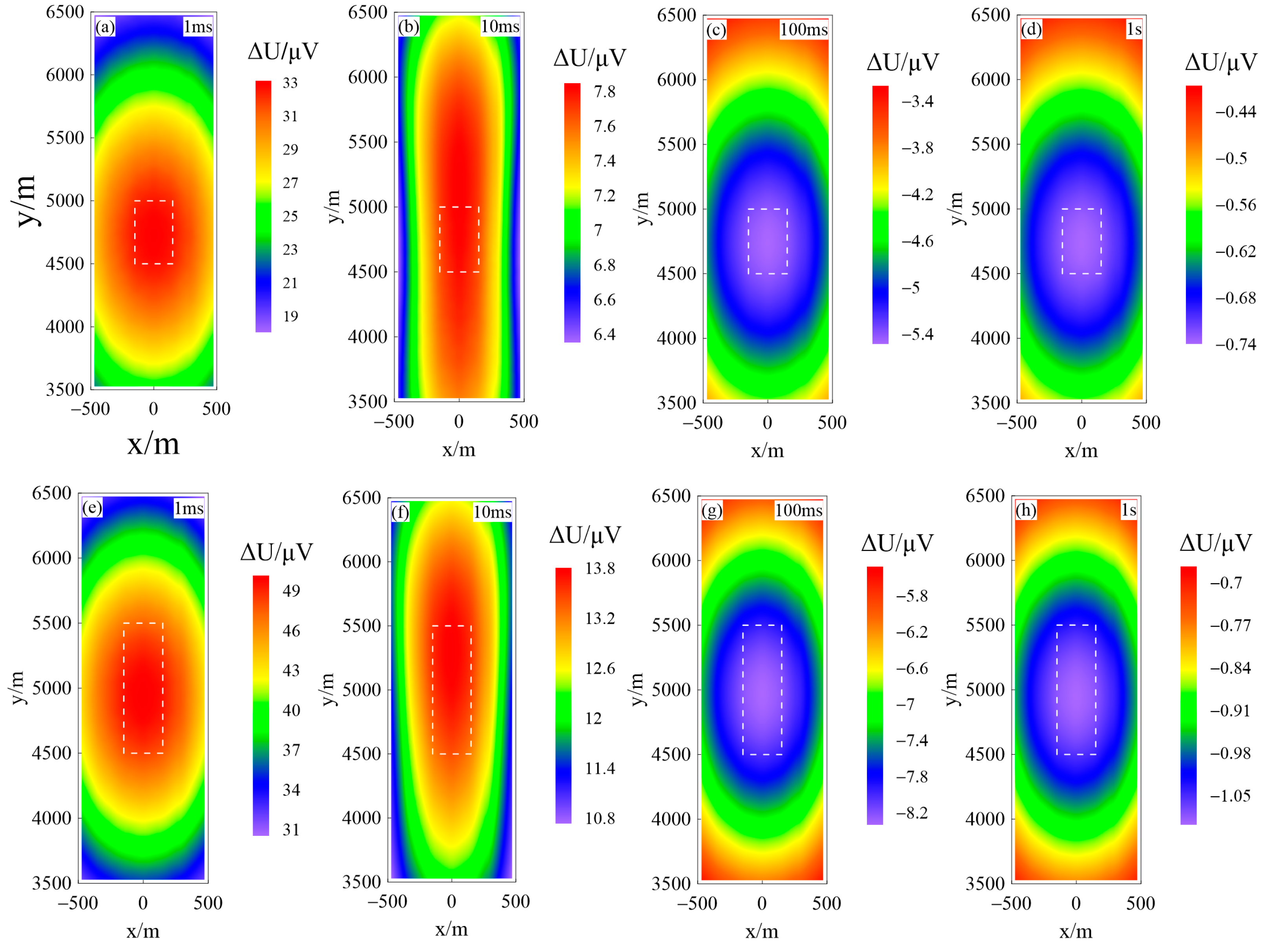
Forward modeling is a numerical simulation method that simulates the physical phenomena of subsurface media to match the observed results. Its main purpose is to integrate with the actual geological conditions. To simulate the feasibility of the transient electromagnetic considering the IP effect based on SEM in hydraulic fracturing monitoring, this study refers to the well data of Well Jiaoye 30 in the Fuling Shale Gas Field area and designs a physical model of two-stage fracturing (Figure 15). The length of the source is 3000 m, the thickness of the fracturing layer is 300 m, and the fracturing area extends along the y direction by 500 m after each fracturing stage. The resistivity before fracturing is 50 Ω·m, and the IP parameters are all set to 0. After fracturing, the resistivity decreases due to the injection of fracturing fluid, assuming the resistivity decreases to 5 Ω·m, with a polarizability of 0.5 and a time constant of 1. Figure 16a–d show the contour maps of the voltage difference at 1 ms, 10 ms, 100 ms, and 1 s time channels before and after the first-stage fracturing, while Figure 16e–h show the contour maps of the voltage difference at 1 ms, 10 ms, 100 ms, and 1 s time channels before and after the second-stage fracturing. From the figures, it can be observed that the fracturing range in the xy plane at each time channel varies due to the attenuation of the electromagnetic signal over time. The reverse voltage appears after 100 ms, and the fracturing area is displayed most accurately. In addition, it can be observed that the overall voltage difference values after the second-stage fracturing are higher than those after the first-stage fracturing in the same time channel. The stronger the signal, the easier it is for the instrument to capture the electromagnetic response of multiple fracturing stages. These results indicate the promising application of the TEM time domain spectral element method considering the IP effect in shale gas fracturing detection.

Figure 15.
Shale gas fracture monitoring model (The red area represents the first fracturing zone, and the green area represents the second fracturing zone).
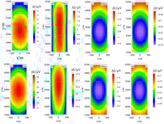
Figure 16.
Contour map of voltage difference at different time steps before and after hydraulic fracturing (The white dashed box represents the fracturing zone): (a–d) represent the voltage difference before and after first-stage hydraulic fracturing at different time steps of 1 ms, 10 ms, 100 ms, and 1 s; (e–h) represent the voltage difference before and after second-stage hydraulic fracturing at different time steps of 1 ms, 10 ms, 100 ms, and 1 s.
6. Conclusions
This article demonstrates through accuracy validation and comparative experiments with different parameters that the proposed method effectively considers the influence of the IP effects. It shows that the polarization effects have a significant impact on the electric field response, with a more severe negative response observed for higher polarizability. Additionally, the method introduced in this article incorporates the Debye model through the differential form of Ohm’s law and discretizes it directly in the time domain using a variable step-size second-order backward Euler method. This approach avoids errors associated with frequency selection and discretization in frequency domain algorithms, resulting in a more direct and accurate treatment of time domain data. The adoption of the SEM allows for flexible simulation of complex geological models while maintaining a certain level of computational efficiency.
Furthermore, a series of three-dimensional validation experiments reveals promising practical applications of this research in shale gas hydraulic fracturing monitoring and other production scenarios. It provides a reliable reference for subsequent data processing, analysis of induced polarization parameters, and inversion studies. Future research aims to incorporate more comprehensive models of complex resistivity to enhance the analysis of induced polarization parameters. Additionally, there are plans to simulate more complex underground geological conditions to expand the scope of application and improve its prospects.
Author Contributions
Conceptualization, X.Z., L.Y. and X.H.; Methodology, X.Z., L.Y. and X.H.; Resources, L.Y., X.H., L.Z. and X.C.; Software, X.Z. and X.W.; Supervision, L.Y. and X.C.; Writing—original draft, X.Z.; Writing—review and editing, L.Y., X.H. and X.C. All authors have read and agreed to the published version of the manuscript.
Funding
This paper is financially supported by the National Natural Science Foundation of China (42030805, 42104070, 42274103, 42374096), the Natural Science Foundation Project of Hubei province (2022CFB229), the Open Fund of Key Laboratory of Exploration Technologies for Oil and Gas Resources (Yangtze University), the Ministry of Education (PI2023-02), and the Guided Project of Scientific Research Program of Hubei Provincial Department of Education: B2019037.
Data Availability Statement
The data presented in this study are available on request from the corresponding author.
Conflicts of Interest
The authors declare no conflict of interest.
References
- Xue, G.Q.; Li, X.; Di, Q.Y. Research progress in TEM forward modeling and inversion calculation. Prog. Geophys. 2008, 23, 1165–1172. [Google Scholar]
- Song, X.J.; Dang, R.R.; Guo, B.L.; Wang, X.L. Research on transient electromagnetic response of magnetic source in borehole. Chin. J. Geophys. 2011, 54, 1122–1129. [Google Scholar]
- Li, Q.L.; Kang, H.M.; Wang, G.J.; Yu, L.J.; Zhu, J.H.; Wang, R.; Zhang, Y.C.; Cao, W.J. Study on the TEM response forward calculation of uniform half-space pulse current. Prog. Geophys. 2023, 38, 1152–1160. [Google Scholar]
- Strack, K.M. The deep transient electromagnetic sounding technique: First field test in Australia. Explor. Geophys. 1984, 15, 251–259. [Google Scholar] [CrossRef]
- Yan, L.J.; Hu, W.B.; Yang, S.H.; Zhang, X.; Jin, Z.F.; Chen, Q.L.; Su, Z.L.; Zheng, R.S.; Hu, J.H. Electromagnetic Exploration Methods and Their Applications in Southern Carbonate Rock Regions; Petroleum Industry Press: Beijing, China, 2001. [Google Scholar]
- Chen, J.L.; Wang, H.J.; Xu, Z.Z.; Huang, Q.S.; Jiang, G.Q. Research on aquifer water abundance evaluation by borehole transient electromagnetic method based on FCNN. Coal Geol. Explor. 2023, 51, 289–297. [Google Scholar]
- Yang, H.K. Hydrogeological exploration technology for the Longdong coal mine goaf based on the transient electromagnetic method. Geol. Explor. 2023, 59, 883–890. [Google Scholar]
- Xiong, Z.H. Electromagnetic modeling of 3D structures by the method of system iteration using integral equations. Geophysics 1992, 57, 1556–1561. [Google Scholar] [CrossRef]
- Zhdanov, M.S.; Lee, S.K.; Yoshioka, K. Integral equation method for 3D modeling of electromagnetic fields in complex structures with inhomogeneous background conductivity. Geophysics 2006, 71, G333–G345. [Google Scholar] [CrossRef]
- Cox, L.H.; Wilson, G.A.; Zhdanov, M.S. 3D inversion of airborne electromagnetic data using a moving footprint. Explor. Geophys. 2010, 41, 250–259. [Google Scholar] [CrossRef]
- Avdeev, D.B. Three-dimensional electromagnetic modeling and inversion from theory to application. Surv. Geophys. 2005, 26, 767–799. [Google Scholar] [CrossRef]
- Liu, Y.H.; Yin, C.C. 3D anisotropic modeling for airborne EM systems using finite-difference method. J. Appl. Geophys. 2014, 109, 186–194. [Google Scholar] [CrossRef]
- Wang, W.P.; Zeng, Z.F.; Li, J.; Wu, C.P. Top graphic Effects and Correction for frequency airborne electromagnetic method. J. Jilin Univ. Earth Sci. Ed. 2015, 45, 941–951. [Google Scholar]
- Sun, H.F.; Liu, S.B.; Yang, Y. Crank-Nicolson FETD 3D forward modeling for the transient electromagnetic field. Chin. J. Geophys. 2021, 64, 343–354. [Google Scholar]
- Cai, H.; Čuma, M.; Zhdanov, M.S. Three-dimensional parallel edge-based finite element modeling of electromagnetic data with field redatuming. In SEG Technical Program Expanded Abstracts; Society of Exploration Geophysicists: Houston, TX, USA, 2015; pp. 1012–1017. [Google Scholar]
- Zhang, B. Research on Finite-Element Method Based on Unstructured Grids for Airborne EM Modeling. Ph.D. Thesis, Jilin University, Changchun, China, 2017. [Google Scholar]
- Wang, X.Y.; Yan, L.J.; Mao, Y.R.; Huang, X.; Xie, X.B.; Zhou, L. Three-dimensional forward modeling of long-offset transient electromagnetic method over topography. J. Jilin Univ. Earth Sci. Ed. 2022, 52, 754–765. [Google Scholar]
- Wang, X.Y.; Wang, C.; Mao, Y.R.; Yan, L.J.; Zhou, L.; Gao, W.L. 3D forward modeling of DC resistivity method based on finite element with mixed grid. Coal Geol. Explor. 2022, 50, 136–143. [Google Scholar]
- Haber, E.; Ascher, U.M. Fast finite volume simulation of 3D electromagnetic problems with highly discontinuous coefficients. SIAM J. Sci. Comput. 2001, 22, 1943–1961. [Google Scholar] [CrossRef]
- Jahandari, H.; Farquharson, G.C. Finite-volume modelling of geophysical electromagnetic data on unstructured grids using potentials. Geophys. J. Int. 2015, 202, 1859–1876. [Google Scholar] [CrossRef]
- Mata, L.C.; Haber, E.; Schwarzbach, C. An oversampling technique for multiscale finite volume method to simulate frequency-domain electromagnetic responses. In Proceedings of the SEG Technical Program Expanded Abstracts, Dallas, TX, USA, 16–21 October 2016; pp. 981–985. [Google Scholar]
- Lee, J.H.; Xiao, T.; Liu, Q.H. A 3-D spectral-element method using mixed-order curl conforming vector basis functions for electromagnetic fields. IEEE Trans. Microw. Theory Tech. 2006, 54, 437–444. [Google Scholar]
- Huang, Y.; Chen, J.F.; Zhang, J.J.; Liu, Q.H. A parallel high precision integration scheme with spectral element method for transient electromagnetic computation. In Proceedings of the Digests of the 2010 14th Biennial IEEE Conference on Electromagnetic Field Computation, Chicago, IL, USA, 9–12 May 2010; p. 1. [Google Scholar]
- Zhou, Y.G.; Zhuang, M.W.; Shi, L.L.; Cai, X.G.; Liu, N.; Liu, Q.H. Spectral-element method with divergence-free constraint for 2.5-D marine CSEM hydrocarbon exploration. IEEE Geosci. Remote Sens. Lett. 2017, 14, 1973–1977. [Google Scholar] [CrossRef]
- Huang, X. 3D Frequency-Domain/Time-Domain Airborne EM forward Modeling Based on Spectral-Element Method with Arbitrary Hexahedral Grids. Ph.D. Thesis, Jilin University, Changchun, China, 2019. [Google Scholar]
- Nie, Z.F.; Tao, C.H.; Shen, J.S.; Zhu, Z.M. 3D transient electromagnetics forward modeling with complex topography and structure: A case study of the TAG hydrothermal field, Mid-Atlantic Ridge. Haiyang Xuebao 2021, 43, 145–156. [Google Scholar]
- Liu, S.B.; Sun, H.F.; Li, W.H.; Wang, Z.; Yang, Y. 3D transient electromagnetics forward modeling using BEDS-FDTD and its stability verification. Chin. J. Geophys. 2023, 66, 841–853. [Google Scholar]
- Zhou, J.M.; Jing, X.; Lu, K.L.; Liu, W.T.; Li, X. Three-dimensional full-time transient electromagnetic modeling using restarting polynomial Krylov subspace model order reduction method. Chin. J. Geophys. 2023, 66, 2646–2657. [Google Scholar]
- Xiang, K.; Yan, L.J.; Hu, H.; Hu, W.B.; Tang, X.G.; Liu, X.J. Relationship analysis between brittle index and electrical properties of marine shale in South China. Geophys. Prospect. Pet. 2016, 55, 894–903. [Google Scholar]
- Tong, X.L.; Yan, L.j.; Xiang, K. Analysis of low-frequency complex resistivity characteristics under formation conditions. Geophys. Prospect. Pet. 2020, 59, 472–480. [Google Scholar]
- Spies, B.R. A field occurrence of sign reversals with the transient electromagnetic method. Geophys. Prospect. 1980, 28, 620–632. [Google Scholar] [CrossRef]
- Weidelt, P. Response characteristics of coincident loop transient electromagnetic systems. Geophysics 1982, 47, 1325–1330. [Google Scholar] [CrossRef]
- Man, K.F. Forward Modeling and Inversion of Induced Polarization Parameters from Time-Domain Airborne EM Data. Ph.D. Thesis, Jilin University, Changchun, China, 2021. [Google Scholar]
- Zhang, X.C.; Yin, C.C. Forward modeling of airborne EM induced polarization effect in time domain based on Debye model. J. Jilin Univ. Earth Sci. Ed. 2023, 53, 4710–4719. [Google Scholar]
- Li, L.; Wang, P. Study on characteristics of multiple “symbol reversal” phenomena of grounded-wiresource transient electromagnetic decay response curve. Comput. Tech. Geophys. Geochem. Explor. 2020, 42, 773–781. [Google Scholar]
- Li, L.; Feng, K.; Tu, J.; Li, W.L.; Yang, C. Influence of IP effect on grounded-wire TEM response. Comput. Tech. Geophys. Geochem. Explor. 2019, 41, 639–641. [Google Scholar]
- Li, L. Study on Forward and Inversion Algorithm of Grounded Source Transient Electromagnetic with IP Effects. Master’s Thesis, Chengdu University of Technology, Chengdu, China, 2019. [Google Scholar]
- Liu, M.H.; Cai, H.Z.; Yang, H.; Xiong, Y.C.; Hu, X.Y. Three-dimensional joint inversion of ground and semi-airborne transient electromagnetic method. Chin. J. Geophys. 2022, 65, 3997–4011. [Google Scholar]
- Debye, P.; Falkenhagen, H. Dispersion of the Conductivity and Dielectric Constants of Strong Electrolytes. Phys. Z. 1928, 29, 401–426. [Google Scholar]
- Cole, K.S.; Cole, R.H. Dispersion and absorption in dielectrics I. Alternating current characteristics. J. Chem. Phys. 1941, 9, 341–351. [Google Scholar] [CrossRef]
- Wait, J.R. Chapter 3-A phnonmenological theory over voltage for metallic particles. In Over Voltage Research and Geophysical Applications; Elsevier Ltd.: Amsterdam, The Netherlands, 1959. [Google Scholar]
- Dias, C.A. Analytical model for a polarizable medium at radio and lowerfrequencies. J. Geophys. Res. Atmos. 1972, 77, 4945–4956. [Google Scholar] [CrossRef]
- Zhdanov, M.S. Generalized effective medium theory of induced polarization. SEG Tech. Program Expand. Abstr. 2006, 25, 805–809. [Google Scholar]
- Zhdanov, M.S. Generalized effective medium theory of induced polarization. Geophysics 2008, 73, 197–211. [Google Scholar] [CrossRef]
- Zonge, K.L.; Soke, N.A.; Sumner, J.S. Comparison of time, frequency and phase measurements in IP. Geophys. Prospect. 1972, 20, 626–628. [Google Scholar] [CrossRef]
- Wu, Y.Q. Three-Dimensional Time-Domain Electromagnetic Response Numerical Simulation and Intelligent Identification of Polarization Media. Ph.D. Thesis, Jilin University, Changchun, China, 2021. [Google Scholar]
- Yang, J. Grounded Wire Source Transient Electromagnetic Confinement Inversion Based on Polarized Media and Applications. Master’s Thesis, Yangtze University, Wuhan, China, 2023. [Google Scholar]


Disclaimer/Publisher’s Note: The statements, opinions and data contained in all publications are solely those of the individual author(s) and contributor(s) and not of MDPI and/or the editor(s). MDPI and/or the editor(s) disclaim responsibility for any injury to people or property resulting from any ideas, methods, instructions or products referred to in the content. |
© 2023 by the authors. Licensee MDPI, Basel, Switzerland. This article is an open access article distributed under the terms and conditions of the Creative Commons Attribution (CC BY) license (https://creativecommons.org/licenses/by/4.0/).