
Targeting Paleovalley-Related Ferricrete Units in Yilgarn Craton Using High-Resolution Aeromagnetic Data and Spatial Machine Learning

 ,
,  ,
,
Abstract
:1. Introduction
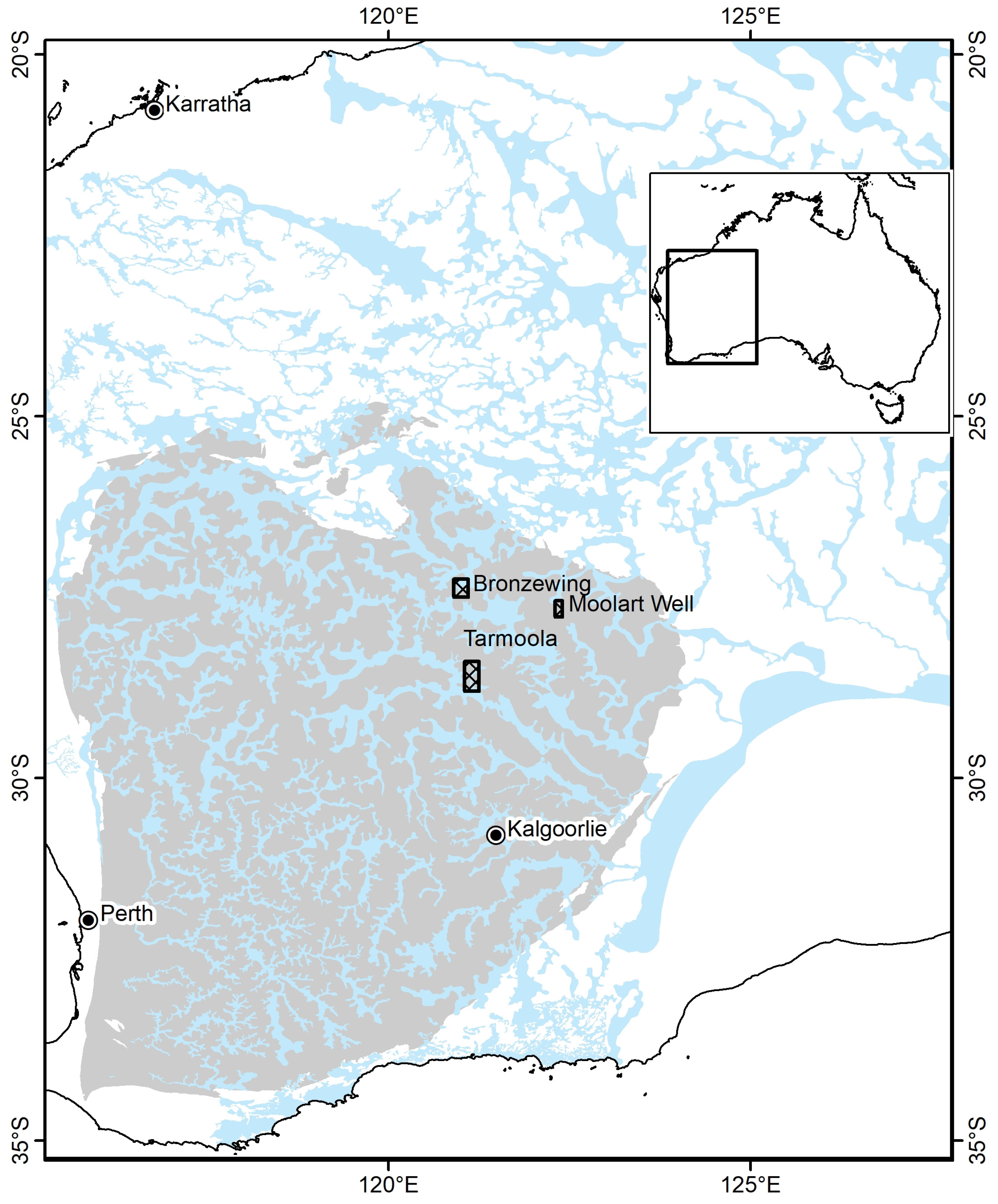
2. Study Areas
2.1. Tarmoola
2.2. Bronzewing
2.3. Moolart Well
3. Materials and Methods
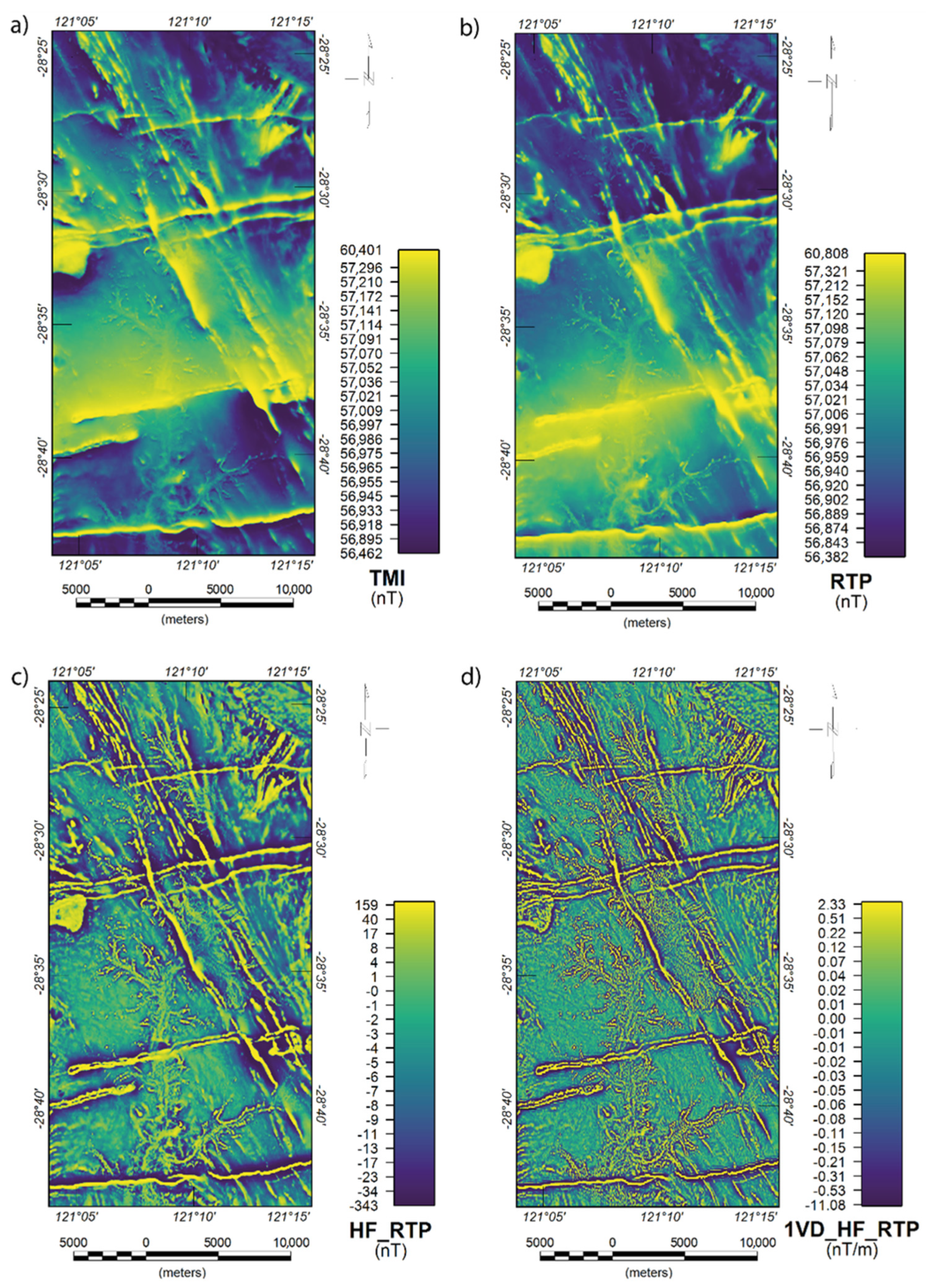
3.1. High-Resolution Aeromagnetic Data
3.2. Spatial Machine Learning
3.3. Model Training
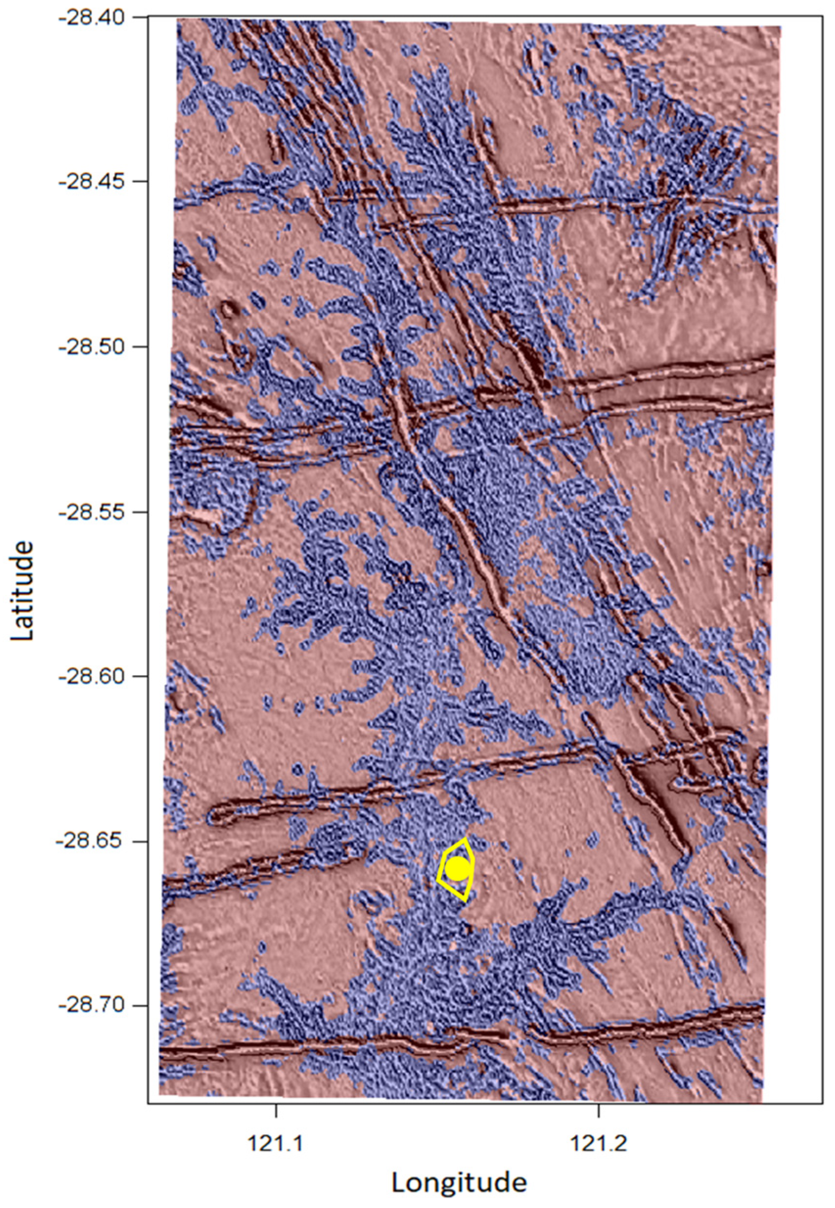
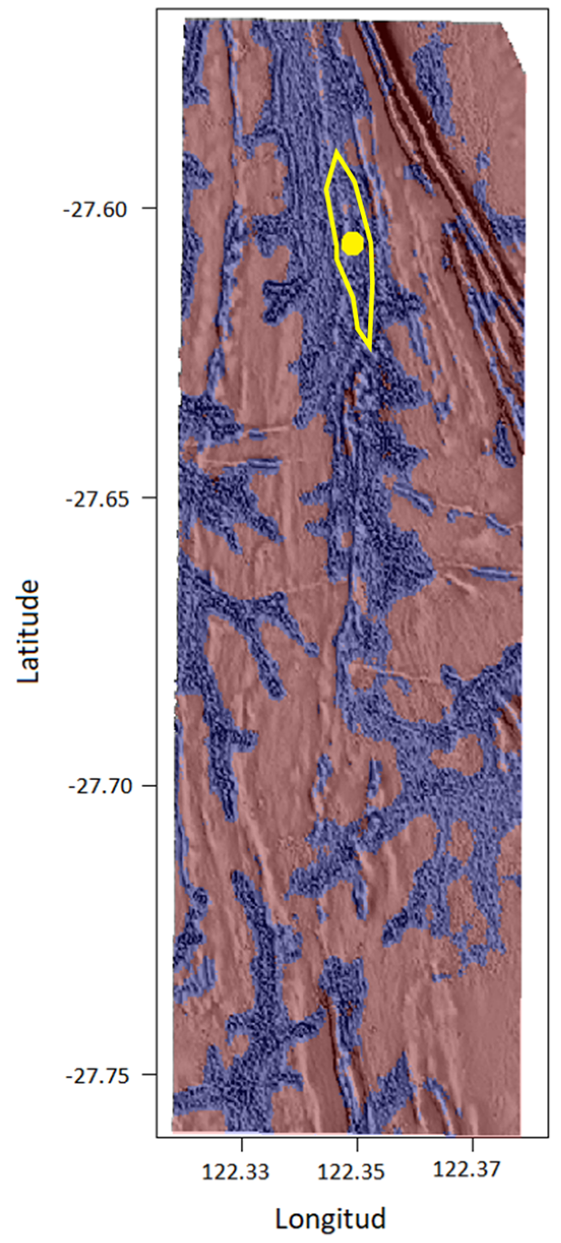
4. Results
4.1. Tarmoola
4.2. Bronzewing
4.3. Moolart Well
5. Discussion
6. Conclusions
Author Contributions
Funding
Data Availability Statement
Acknowledgments
Conflicts of Interest
References
- Lamplugh, G.W. Calcrete. Geol. Mag. 1902, 9, 575. [Google Scholar] [CrossRef] [Green Version]
- Anand, R.R.; Paine, M. Regolith Geology of the Yilgarn Craton, Western Australia: Implications for Exploration. Aust. J. Earth Sci. 2002, 49, 3–162. [Google Scholar] [CrossRef]
- Anand, R.R.; Hough, R.M.; Salama, W.; Aspandiar, M.F.; Butt, C.R.M.; González-Álvarez, I.; Metelka, V. Gold and Pathfinder Elements in Ferricrete Gold Deposits of the Yilgarn Craton of Western Australia: A Review with New Concepts. Ore Geol. Rev. 2019, 104, 294–355. [Google Scholar] [CrossRef]
- Anand, R.R.; Lintern, M.; Hough, R.; Noble, R.; Verrall, M.; Salama, W.; Balkau, J.; Radford, N. The Dynamics of Gold in Regolith Change with Differing Environmental Conditions over Time. Geology 2017, 45, 127–130. [Google Scholar] [CrossRef]
- Galloway Warland, N.; Phang, C. Laterite Gold Deposits-Southern Yandal Belt. In Yandal Greenstone Belt Regolith, Geology and Mineralisation; AIG Bulletin No. 32; Phillips, G.N., Anand, R.R., Eds.; Australian Institute of Geoscientists Bulletin: Perth, Australia, 2000; pp. 179–186. [Google Scholar]
- Paine, M.D.; Foo, M.F.P.; Phang, C.; Cox, A. Description and Evolution of the Gourdis and Empire Laterite Gold Deposits, Northern Yandal Belt. In Proceedings of the Yandal Greenstone Belt, Perth, Australia, 10–11 July 2000; Phillips, G.N., Anand, R.R., Eds.; AIG Bulletin No. 32. Australian Institute of Geoscientists: Perth, Australia, 2000; pp. 165–177. [Google Scholar]
- Anand, R.R. Regolith and Geochemical Synthesis of the Yandal Greenstone Belt. In Proceedings of the Yandal Greenstone Belt, Perth, Australia, 10–11 July 2000; Phillips, G.N., Anand, R.R., Eds.; AIG Bulletin No. 32. Australian Institute of Geoscientists: Perth, Australia; 2000; pp. 79–111. [Google Scholar]
- Jones, M.; Lidbury, R. Unconformity-Related Weathered Laterite Profiles at Mt Gibson Gold Mine, Yilgarn Craton, Western Australia. In New Approaches to an Old Continent, Proceedings of the 3rd Australian Regolith Conference, Kalgoorlie, Australia, 2–9 May 1998; Britt, A.F., Bettenay, L., Eds.; CRC Leme: Glen Osmond, Australia, 1998. [Google Scholar]
- De Broekert, P. Origin of Tertiary Inset-Valleys and Their Fills, Kalgoorlie, Western Australia. Ph.D. Thesis, Australian National University, Canberra, Australia, 2002. [Google Scholar]
- Kern, A.M.; Commander, D.P. Cainozoic Stratigraphy in the Roe Palaeodrainage of the Kalgoorlie Region, Western Australia. Geol. Surv. West. Aust. Rep. 1993, 34, 85–95. [Google Scholar]
- Clarke, J.D.A. Stratigraphy of the Lefroy and Cowan Palaeodrainages, Western Australia. J. R. Soc. West. Aust. 1993, 76, 15–22. [Google Scholar]
- De Broekert, P.; Sandiford, M. Buried Inset-Valleys in the Eastern Yilgarn Craton, Western Australia: Geomorphology, Age, and Allogenic Control. J. Geol. 2005, 113, 471–493. [Google Scholar] [CrossRef] [Green Version]
- Thorne, R.; Anand, R.; Suvorova, A. The Formation of Fluvio-Lacustrine Ferruginous Pisoliths in the Extensive Palaeochannels of the Yilgarn Craton, Western Australia. Sediment. Geol. 2014, 313, 32–44. [Google Scholar] [CrossRef]
- Wildman, J.E.; Compston, D. Magnetic Expression of Palaeodrainage Systems in the Yandal Greenstone Belt: Implications for Exploration. In Yandal Greenstone Belt, Regolith, Geology and Mineralisation; AIG Bulletin No. 32; Australian Institute of Geoscientists: Perth, Australia, 2000; pp. 157–164. [Google Scholar]
- Foss, C.; Reed, G.; Keeping, T.; Davies, M. Magnetic Mapping of River Channel and Palaeochannel Deposits—An Example from Teetulpa, South Australia. ASEG Ext. Abstr. 2015, 2015, 1–4. [Google Scholar] [CrossRef] [Green Version]
- Mackey, T.; Lawrie, K.; Wilkes, P.; Munday, T.; de Souza Kovacs, N.; Chan, R.; Gibson, D.; Chartres, C.; Evans, R. Palaeochannels near West Wyalong, New South Wales: A Case Study in Delineation and Modelling Using Aeromagnetics. Explor. Geophys. 2000, 31, 1–7. [Google Scholar] [CrossRef]
- Jessell, M.; Boamah, K.; Duodu, J.A.; Ley-Cooper, Y. Geophysical Evidence for a Major Palaeochannel within the Obosum Group of the Volta Basin, Northern Region, Ghana. J. Afr. Earth Sci. 2015, 112, 586–596. [Google Scholar] [CrossRef]
- Wilford, J. Using Airborne Geophysics to Define the 3D Distribution and Landscape Evolution of Quaternary Valley-Fill Deposits around the Jamestown Area, South Australia. Aust. J. Earth Sci. 2009, 56, S67–S88. [Google Scholar] [CrossRef]
- Anand, R.R.; Gilkes, R.J. The Association of Maghemite and Corundum in Darling Range Laterites, Western Australia. Soil Res. 1987, 25, 303–311. [Google Scholar] [CrossRef]
- Bergen, K.J.; Johnson, P.A.; de Hoop, M.V.; Beroza, G.C. Machine Learning for Data-Driven Discovery in Solid Earth Geoscience. Science 2019, 363, eaau0323. [Google Scholar] [CrossRef]
- Talebi, H.; Mueller, U.; Tolosana-Delgado, R.; Grunsky, E.C.; McKinley, J.M.; Caritat, P. Surficial and Deep Earth Material Prediction from Geochemical Compositions. Nat. Resour. Res. 2019, 28, 869–891. [Google Scholar] [CrossRef] [Green Version]
- Zuo, R.; Xiong, Y.; Wang, J.; Carranza, E.J.M. Deep Learning and Its Application in Geochemical Mapping. Earth-Sci. Rev. 2019, 192, 1–14. [Google Scholar] [CrossRef]
- Talebi, H.; Mueller, U.; Peeters, L.J.M.; Otto, A.; de Caritat, P.; Tolosana-Delgado, R.; van den Boogaart, K.G. Stochastic Modelling of Mineral Exploration Targets. Math. Geosci. 2022, 54, 593–621. [Google Scholar] [CrossRef]
- Schaeben, H.; Kost, S.; Semmler, G. Popular Raster-Based Methods of Prospectivity Modeling and Their Relationships. Math. Geosci. 2019. [Google Scholar] [CrossRef]
- Sun, T.; Li, H.; Wu, K.; Chen, F.; Zhu, Z.; Hu, Z. Data-Driven Predictive Modelling of Mineral Prospectivity Using Machine Learning and Deep Learning Methods: A Case Study from Southern Jiangxi Province, China. Minerals 2020, 10, 102. [Google Scholar] [CrossRef] [Green Version]
- Lary, D.J.; Alavi, A.H.; Gandomi, A.H.; Walker, A.L. Machine Learning in Geosciences and Remote Sensing. Geosci. Front. 2016, 7, 3–10. [Google Scholar] [CrossRef] [Green Version]
- Wang, Z.; Di, H.; Shafiq, M.A.; Alaudah, Y.; AlRegib, G. Successful Leveraging of Image Processing and Machine Learning in Seismic Structural Interpretation: A Review. Lead. Edge 2018, 37, 451–461. [Google Scholar] [CrossRef]
- Talebi, H.; Peeters, L.J.M.; Mueller, U.; Tolosana-Delgado, R.; van den Boogaart, K.G. Towards Geostatistical Learning for the Geosciences: A Case Study in Improving the Spatial Awareness of Spectral Clustering. Math. Geosci. 2020, 52, 1035–1048. [Google Scholar] [CrossRef]
- Karpatne, A.; Ebert-Uphoff, I.; Ravela, S.; Babaie, H.A.; Kumar, V. Machine Learning for the Geosciences: Challenges and Opportunities. IEEE Trans. Knowl. Data Eng. 2019, 31, 1544–1554. [Google Scholar] [CrossRef] [Green Version]
- Lecun, Y.; Bottou, L.; Bengio, Y.; Haffner, P. Gradient-Based Learning Applied to Document Recognition. Proc. IEEE 1998, 86, 2278–2324. [Google Scholar] [CrossRef] [Green Version]
- LeCun, Y.; Bengio, Y.; Hinton, G. Deep Learning. Nature 2015, 521, 436–444. [Google Scholar] [CrossRef]
- Talebi, H.; Peeters, L.J.M.; Otto, A.; Tolosana-Delgado, R. A Truly Spatial Random Forests Algorithm for Geoscience Data Analysis and Modelling. Math. Geosci. 2022, 54, 1–22. [Google Scholar] [CrossRef]
- Bell, J.; Kilgour, P.; English, P.; Woodgate, M.; Lewis, S.; Wischusen, J. WASANT Palaeovalley Map—Distribution of Palaeovalleys in Arid and Semi-Arid WA-SA-NT (First Edition), Scale: 1:4 500 000. Geoscientific Thematic Map (Geocat No 73980); Geoscience Australia: Canberra, Australia, 2012. [Google Scholar]
- Balkau, J.; Walker, D.; McCracken, S.; Hawker, A.; Carver, R.; Taylor, T.; Ion, J. The discovery and resource development of the Moolart Well gold deposit, Western Australia. In Proceedings of the New Generation of Gold Mines Conference, Perth, Australia, 15–16 November 2007; Paydirt Media Pty. Ltd.: Perth, Australia, 2007; pp. 833–855. [Google Scholar]
- Blakely, R.J. Potential Theory in Gravity and Magnetic Applications; Cambridge University Press: New York, NY, USA, 1996. [Google Scholar]
- Briggs, I.C. Machine Contouring Using Minimum Curvature. Geophysics 1974, 39, 39–48. [Google Scholar] [CrossRef]
- Nabighian, M.N. The Analytic Signal of Two-Dimensional Magnetic Bodies with Polygonal Cross-Section: Its Properties and Use for Automated Anomaly Interpretation. Geophysics 1972, 37, 507–517. [Google Scholar] [CrossRef]
- Dentith, M.; Mudge, S.T. Geophysics for the Mineral Exploration Geoscientist; Cambridge University Press: Cambridge, UK, 2014. [Google Scholar]
- Probst, P.; Wright, M.N.; Boulesteix, A. Hyperparameters and Tuning Strategies for Random Forest. WIREs Data Min. Knowl. Discov. 2019, 9, e1301. [Google Scholar] [CrossRef] [Green Version]


| Area | Survey Name | Flying Height (m) | Line Spacing (m) | Company | Contractor | Year |
|---|---|---|---|---|---|---|
| Moolart Well | Duketon | 20 | 50 | Newmont Australia Ltd. | UTS Geophysics | 2003 |
| Tarmoola | Leonora | 50 | 100 | CGG Aviation Aus | Tesla Airborne Geoscience | 1996 |
| Bronzewing | Bronzewing Area | 25 | 50 | Great Central Mines Ltd. | UTS Geophysics | 1998 |
| Mt McClure 97 | 35 | 50 | Arimco Mining Co., Ltd. | Tesla Airborne Geoscience | 1997 | |
| Mount Joel | 25 | 50 | Great Central Mines Ltd. | UTS Geophysics | 1996 | |
| Bronzewing South | 20 | 50 | Newmont Australia Ltd. | UTS Geophysics | 2003 |
| Transformation | Description | Purpose | Disadvantage | Reference |
|---|---|---|---|---|
| Reduction to pole (RTP) | Removes asymmetrical influence of the ambient magnetic field and reproduces magnetic anomalies assuming vertical inducing field | In the vertical ambient field magnetic anomalies are easier to understand. Magnetic bodies with positive susceptibility contrast will appear under the positive magnetic anomalies | The transformation will fail in the presence of the remanent magnetisation, if not accounted for | [37] |
| First Vertical Derivative (1VD) | Produces maximum rate of the change of the magnetic field in the vertical direction | Used to emphasise high frequency, usually shallow magnetic sources | Can highlight noise or survey artifacts | [38] |
| Upward Continuation (UC) | Reproduces magnetic anomalies at the higher designated height | Reducing amplitude of near-surface magnetic anomalies | If a survey was draped over topography, piecewise UC should be applied, which can introduce processing artifacts and misrepresent high-frequency features | [35,38] |
| Predicted | Class Error | ||
|---|---|---|---|
| Observed | 1 | 0 | |
| 1 | 473 | 27 | 5.4% |
| 0 | 54 | 446 | 10.8% |
| Predicted | Class Error | ||
|---|---|---|---|
| Observed | 1 | 0 | |
| 1 | 423 | 77 | 15.4% |
| 0 | 98 | 402 | 19.6% |
| Predicted | Class Error | ||
|---|---|---|---|
| Observed | 1 | 0 | |
| 1 | 469 | 31 | 6.2% |
| 0 | 49 | 451 | 9.8% |
Publisher’s Note: MDPI stays neutral with regard to jurisdictional claims in published maps and institutional affiliations. |
© 2022 by the authors. Licensee MDPI, Basel, Switzerland. This article is an open access article distributed under the terms and conditions of the Creative Commons Attribution (CC BY) license (https://creativecommons.org/licenses/by/4.0/).
Share and Cite
Talebi, H.; Markov, J.; Salama, W.; Otto, A.; Metelka, V.; Anand, R.; Cole, D. Targeting Paleovalley-Related Ferricrete Units in Yilgarn Craton Using High-Resolution Aeromagnetic Data and Spatial Machine Learning. Minerals 2022, 12, 879. https://doi.org/10.3390/min12070879
Talebi H, Markov J, Salama W, Otto A, Metelka V, Anand R, Cole D. Targeting Paleovalley-Related Ferricrete Units in Yilgarn Craton Using High-Resolution Aeromagnetic Data and Spatial Machine Learning. Minerals. 2022; 12(7):879. https://doi.org/10.3390/min12070879
Chicago/Turabian StyleTalebi, Hassan, Jelena Markov, Walid Salama, Alex Otto, Vasek Metelka, Ravi Anand, and Dave Cole. 2022. "Targeting Paleovalley-Related Ferricrete Units in Yilgarn Craton Using High-Resolution Aeromagnetic Data and Spatial Machine Learning" Minerals 12, no. 7: 879. https://doi.org/10.3390/min12070879
APA StyleTalebi, H., Markov, J., Salama, W., Otto, A., Metelka, V., Anand, R., & Cole, D. (2022). Targeting Paleovalley-Related Ferricrete Units in Yilgarn Craton Using High-Resolution Aeromagnetic Data and Spatial Machine Learning. Minerals, 12(7), 879. https://doi.org/10.3390/min12070879