Abstract
The Tinto and Odiel rivers (SW Spain) drain from a vast sulfide mining district and join at a 20-km-long estuary that enters the Atlantic Ocean. In this work, the contents of rare earth elements (REE) and fractionation in Neogene–Holocene sediment cores from La Fontanilla cove (Tinto estuary) were studied. The sediments were collected from a depth of 18 m at different distances from the recent river flow and were analyzed for new information on the temporal development of the REE load in the sediment column. Results show that the ∑ REE is higher in the finer sediments and during periods of mining activity from prehistoric to recent times. Marine influence appears to increase the light REE (LREE) relative to the heavy REE (HREE). The REE patterns of these estuarine sediments show convex curvatures in the MREE relative to the LREE and HREE, indicating the presence of acid-mixing processes between the fluvial waters affected by acid mine drainage (AMD) and seawater, as well as the precipitation of poorly crystalline mineral phases. Significant positive Eu anomalies were found in ebb-tide channels and marsh deposits, which can reflect the mineralogical composition and/or a strong localized salinity gradient combined with organic matter degradation. Sedimentological characteristics of the deposits appear to play the main role in accumulation and fractionation of the REE.
1. Introduction
The rare earth elements (REE, from La to Lu) with largely coherent chemical properties have been used to glean understanding of many geological and environmental processes. These applications rely on examining fractionation within the REE and/or the behavior of individual REE. Increased stability of the heavy rare earths (HREE) in aqueous complexes results in the HREE complexing more readily and remaining in solution [1,2,3], whereas the light rare earths (LREE) will more readily adsorb on particle surfaces [4,5]. The differences in ionic radius, oxidation state, and bonding of the REE drive fractionation of these elements in natural systems. REE typically exhibit trivalent oxidation states. Cerium may also occur as Ce4+, and europium as Eu2+.
REE chemistry in estuarine sediments is controlled by physical and chemical processes [5,6,7,8]. Cerium enrichment or depletion in sediments, relative to the neighboring La and Pr, may occur. Nevertheless, it should be noted that lower stability of the surface complexes of La in seawater may lead to a spurious false negative of Ce/Ce* [9,10,11] due to the possible anomalous abundance of La in estuaries with a significant influence on the marine environment. Eu enrichments in estuarine sediments may also occur due to the slow dissociation rate of Eu–humate complexes at the slightly alkaline pH levels found in estuaries [6,12,13,14]. The shape and size of an estuary, as well as the sediment type (sandy vs. clay-rich), influence sediments’ REE chemistry.
Rivers are considered the chief sources of REE for the ocean [15,16]. The REE compositions of rivers may undergo substantial transformations in estuaries. Here, the non-conservative behavior of REE has been attributed to sea-salt-induced coagulation of colloids, “boundary exchange”, shallow pore water fluxes, submarine groundwater discharge acting along ocean–continent margins, and scavenging with sinking particles in the water column [17,18,19,20,21,22,23]. REE patterns are either inherited from their parent material and controlled by physical and chemical processes [9,24] or from anthropogenic sources [25,26,27].
The majority of publications found in the literature concerning the behavior of REE in estuarine sediments have been made focused on surface samples or short cores (<30 cm depth) [28,29,30,31,32,33,34]. Relatively few studies have considered the behavior of REE (or other sediment constituents) in deeper cores, which would allow for the evaluation of records regarding climate change, contamination, and catastrophic events [35,36,37,38].
In areas affected by mining activities, REE may behave as tracers of acid mine drainage (AMD) contamination. In fact, numerous investigations on the identification of the water–rock interactions that govern the chemistry of AMD were made, and several publications have reported the REE geochemistry of AMD waters in the last two decades [10,39,40,41,42,43,44,45,46,47,48]. These works have reported a shale-normalized pattern enriched in middle REE (MREE) relative to LREE and HREE. Thus, estuarine sediments may be affected by events far upstream that may have taken place thousands of years ago [49,50,51,52]. This is the case for the Tinto–Odiel estuary (SW Spain) studied in the present work. The Tinto and Odiel rivers drain 100 km from the Rio Tinto sulfide mining district and join at a 20-km-long estuary that enters the Atlantic Ocean (Figure 1A,B). In this area, past human activities associated with mining and metallurgy were initiated during the Copper Age [53]. These activities intensified during Roman times, and the decrease/closure in mining exploitation of massive sulfide deposits (e.g., São Domingos, Las Herrerias) only occurred during the second half of the 20th century. The legacy of contamination by these elements, mainly from leaching of the slags and tailings, as well as remobilization/reworking of the contaminated estuarine sediments, is still being recorded in estuarine and marine sediments collected in the southwestern Iberian Atlantic shelf [54,55,56,57].

Figure 1.
(A,B) Location of the study area; (C) location of the cores and main geological and geomorphological features of the bordering areas; (D) lithostratigraphic sections of Core A (inner zone) and Cores B and C (outer zone) showing the location of the studied sample. Data from [52,57,58].
La Fontanilla cove is located in the middle estuary of the Tinto River (Figure 1B,C). On the basis of the sedimentology, geochemistry, paleontology, and dating of three cores collected in this cove (Figure 1: Cores A-B-C) [52,57,58], different sedimentary facies have been distinguished in the Neogene–Holocene evolution of its sedimentary infilling, with a transition from Miocene marine environments to late-Holocene marshes. In this work, the REE data of the three sediments cores collected in this cove are presented.
The specific objectives of the present work are to evaluate (1) the sensitivity of REE to environmental changes in estuarine environments recorded via deep cores; (2) the REE distribution with the depth and its correlation to lithostratigraphic and paleontological analyses; and (3) the REE correlation to prehistoric and historical anthropogenic activities. The main goal is to evaluate, and use, the REE signatures to contribute to the reconstruction of the main environmental changes that occurred in this acid drainage-impacted estuarine environment.
2. Study Area
2.1. The Tinto Estuary
The Tinto River is a small stream (~100 km) that forms a narrow Y-shaped estuary with the Odiel River at its joint mouth in the southwest of the Iberian Peninsula (Figure 1A). This estuary is in an advanced state of clogging, with inner areas made up of wide marshes and barrier islands (Figure 1B: Bacuta Island, Saltés Island). They are protected by two elongated spits (Figure 1B: Punta Umbría, Punta Arenillas) and two jetties. The substrate of these Holocene formations is composed of Miocene silts (Gibraleón Clay Formation) [59], Pliocene silty sands (Huelva Sand Formation) [59], Plio-Pleistocene coarse sands and gravels (Bonares Sand Formation) [60], or Pleistocene fluvial terraces (High Alluvial Level) [61]. During the Pleistocene and Holocene, the fluvial erosion and the Holocene transgression (hereafter referred to as MIS-1 transgression) caused partial dismantling of the Neogene sediments and the creation of small coves, such as La Fontanilla cove (Figure 1B) [58].
The main hydrodynamic processes are controlled by tides and, to a lesser extent, by fluvial discharges, waves, and littoral drift currents. In this estuary, the tidal regime is mesotidal (2.1 m) with a low diurnal inequality [62]. Fluvial discharges are very scarce, varying from minimum flows during very dry years to about 350 Hm3 in rainy years [63]. The wave energy is medium, and 75% of the waves do not exceed 0.5 m in height [64]. The coastal drift currents are oriented towards the east, with a high annual transport of sediment (1.8–3 × 10⁵ m3) [65,66,67]. These currents favor the development of the spits mentioned above and the beaches attached to the east face of the two jetties.
Previous works focused on the mineralogy of sediments of the Tinto–Odiel estuary have shown that the marine Miocene deposits are mainly composed of phyllosilicates (25–47%), quartz (12–28%), feldspars (12–18%), and calcite (5–15%). Overlying alluvial sands and gravels are formed by sand-sized grains of quartz and feldspars within a silty, probably phyllosilicate-rich matrix, and the innermost alluvial sands are coarser than the more external alluvial silty sands; these sediments come mainly from the erosion of the Bonares Sand Formation (quartz: 54–71%; feldspars: 12–18%; phyllosilicates: 11–20%) [68].
One of the main features of the bioclastic silt–sand sediments deposited during the MIS-1 transgression is the presence of significant quantities of shell fragments and valves of bivalves and gastropods. These shells are mostly composed of calcite and, to a lesser extent, aragonite, which increase the carbonate contents of these samples [68].
Concerning clay minerals, smectites are in general absent from the sediments delivered by the Tinto and Odiel rivers into the estuary because their acidic waters are devoid of suspended smectite, due to chemical dissolution induced by the acid mine drainage [69,70]. Illite (70–80%) is the main clay mineral of the recent estuarine sediments, with minor proportions of kaolinite (15–36%) [70].
According to [71], the mineralogical composition of recent sediments at the edge of the tidal channel (Figure 1B: Domingo Rubio channel) is mainly composed of quartz (10–50%), phyllosilicates (40–90%), and feldspars (<15%); subordinate proportions (<5%) of halite and hematite occur. The dominant phyllosilicates are kaolinite and illite, along with dioctahedral smectite in some cases. At the confluence of the estuary with the Tinto River, the presence of vivianite and amorphous iron oxyhydroxides of low structural order was detected; jarosite and gypsum were identified near an uncontrolled deposit of mining waste.
The mineralogical composition of recent sediments obtained by [72] from the Odiel River (a similar provenance area to the sediments of the Tinto River) showed that quartz, feldspars, and phyllosilicates are the major constituents of the bulk sample; the illite–chlorite–kaolinite assemblage found shows the inherited detrital character of the clay minerals. The following heavy minerals were also identified by these authors: magnetite, limonite, goethite, hematite, ilmenite, rutile, pyrite, galena, hornblende, tourmaline, zircon, sphene, apatite, andalusite, sillimanite, distene, epidote, and garnet; these minerals reflect the contributions of different source areas, particularly the Iberian Pyrite Belt and metamorphic rocks.
2.2. Historical and Recent Pollution
The Tinto River crosses the Iberian Pyrite Belt, one of the most important mining provinces in the world. These giant deposits of massive sulfides have been mined for at least 5000 years [64], with two main periods of mining activity: (a) the Roman period (2100-1700 yr BP), with the extraction of more than 20 Mt of polymetallic sulfides [73] and (b) the last 150 years, with an intensive extraction of pyrite and minor quantities of gold and silver. The associated discharges into the riverbed and the washing of its dumps resulted in the generation of AMD. A sharp increase in the oxidation of sulfides is caused by their contact with oxygen and water, releasing acidity and large amounts of sulfates and toxic metals into the river channels. The oxidation of sulfide minerals (mainly pyrite) is accelerated by microbial catalysis, and this process leads to the generation of significant discharges of acid leachates with very high concentrations of toxic elements [74].
This historical pollution has increased with the acidic wastes derived from two industrial concentrations located on the estuarine border (Figure 1B). As a final consequence of all these polluted inputs, the estuary of the Tinto River is one of the most polluted areas in the world, with very high concentrations of As (up to 3000 mg kg−1), Cu (up to 4415 mg kg−1), Pb (up to 10,400 mg kg−1), and Zn (up to 5280 mg kg−1) in its surface sediments [75,76]. Since 1985, this zone has come under a corrective plan for the control of industrial waste disposal.
3. Material and Methods
3.1. Coring and Sampling
Three cores (Figure 1C,D: A-B-C) [48,53,54] were extracted from the old La Fontanilla cove by usual rotary drilling techniques with an almost continuous recovery of sediment and a barrel diameter of 11.6 mm. Core A (18 m depth; 37°13′48″ N-6°53′24″ W) was extracted from the innermost part of this cove. Its paleoenvironmental reconstruction carried out by [52] has revealed a transition from Miocene marine environments to late-Holocene marshes, with an intermediate period that includes alluvial sediments, shallow marine sediments from the MIS-1 transgression, and silty tidal channels and lagoons (~6.5-5.2 kyr BP). Cores B (11.6 m depth; 37°14′ N; 6°54′ W) and C (7.5 m depth; 37°14′06″ N; 6°53′54″ W) were extracted from the outside of this cove, near the Tinto riverbed. The Holocene paleoenvironmental reconstructions of both cores are very similar [57,58], also including the transit from alluvial to marsh deposits and a flood of this outer area during the MIS-1 transgression. The geochemical evolution of both cores includes evidence of early mining activities (~4.5 kyr) and the recent mining period (1870–2001).
Sixty-nine samples (2 cm thickness) were obtained from the three cores (Figure 1D; Core A: 31 samples; Core B: 22 samples; Core C: 16 samples). Selection and distribution of the samples is variable, linked to: (a) the length of each core; (b) the presence of different sedimentary facies; (c) the definition of its limits; and (d) the visual distribution of bioclasts in the cores. Consequently, the number of samples from each core depends on its geological features.
3.2. Compositional Analysis
The trace metal contents of sixty-nine sediment samples (fraction < 2 mm) were performed and certified by MS Analytical, Langley (Canada). Samples were collected manually by handpicking. They were crushed and subsequently ground into powder using an agate mortar. REE contents were obtained by ICP atomic emission spectrometry (total digestion with concentrated acids), with less than 5% variation between different replicate samples and a quality control based on more than 30 sample references (e.g., OREAS 904). In these samples, detection limits vary between 0.01 mg kg−1 (e.g., Ce, Tb, Ho, Tm, Lyu) and 0.1 mg kg−1 (e.g., Nd). A visual analysis of the coarsest sediments has allowed a qualitative evaluation of their main mineral components. Cerium and europium anomalies, e.g., Ce/Ce* and Eu/Eu* values, were calculated from the expressions 2CeN/(LaN+PrN) and 2EuN/(SmN+GdN), respectively.
3.3. Textural Analysis
Grain-size distribution was determined by wet sieving for the coarser fractions with pressured water and floated using sieves of 63, 125, 250, 500, 1000, and 2000 μm diameter. Fractions smaller than 63 μm were analyzed with a particle counter (model Mastersizer-2000) at the CIDERTA center (University of Huelva, Spain). The dispersing agent used was Na-hexametaphosphate.
3.4. Statistical Analysis
The statistical analysis was performed using the R [function cor()] [77]. First, data were standardized due to large differences in the contents of each element. This standardization involves a transformation of the original variables by subtracting their mean and dividing this difference by their standard deviation. The Pearson correlation coefficients were calculated to identify: (i) possible dependence between grain-size distributions and REE and (ii) possible geochemical associations within the REE.
4. Results and Discussion
4.1. Core Descriptions and Paleoenvironmental Significance
The vertical distribution of sedimentary facies is very similar within the three cores, with some minor changes derived from the different geographic location and depth of each core [52,57,58]. The geological substrate of La Fontanilla cove consists of Miocene massive clayey silts with abundant shallow marine assemblages of foraminifera and ostracods. These features allow for placement of these fine sediments inside the upper part of the Gibraleón Clay Formation (Upper Tortonian–Messinian) [59]. This area emerged during the Upper Pliocene–Lower Pleistocene [60], and its substrate was partially dismantled during the Pleistocene, coinciding with a fluvial-dominated period [61]. During the Upper Pleistocene–Middle Holocene, La Fontanilla cove was covered by fluvial and alluvial sediments (Figure 2: see paleoenvironmental interpretation), constituted by silty gravels and brown sands with numerous roots. During the MIS-1 transgression (ca. 6.5–5 kyr BP), this cove was flooded, with the deposition of bioclastic sands and muds (Figure 2: Cores A-B-C). The outer zone of the cove was occupied by phanerogam meadows (Cores B-C), while mesolittoral paleoenvironments are characterized the inner zones (Core A) [78,79]. During the last 5 kyr, this cove emerged progressively, becoming covered by clayey-silty marshes. Finally, the entire area was covered by an anthropic fill at the end of the 20th century.
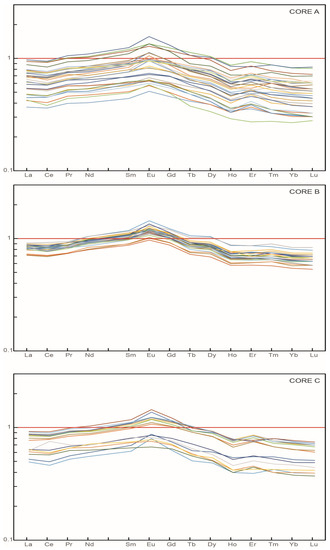
Figure 2.
REE patterns of sediments normalized to PAAS of the samples of the three cores.
4.2. REE and Grain Size
The chemical contents and parameters of REE in the sediments of the three cores of La Fontanilla cove (Tinto estuary, SW Spain) are given in Table 1. The depth of collection and respective paleoenvironment are also given.

Table 1.
Sediment samples’ reference, core, depth, paleoenvironment, REE chemical contents, ∑ REE (sum of total REE, in mg kg−1), LaN/YbN, LaN/SmN, Ce/Ce* and Eu/Eu* ratios (normalized concentrations to PAAS).
The Σ REE (sum of total REE) of the studied sediments are in general lower than those of the Post-Archean Australian average shale (PAAS) [79] and, in most cases, lower than in other fluvial and estuarine systems [80,81,82,83]. The same tendency for low REE concentrations in the surface sediments and in the sediment cores (to a depth of 3.5 m) collected in the Tinto estuary were also found by [41,84]. These low values in the sediments contrast with the previously reported, very high REE concentrations in the dissolved phases of the Tinto estuary water and are related to the low pH values, which prevent particles from adsorbing REE [54].
The variations in REE composition between samples is assessed using the convention of normalization of concentrations to PAAS [79]. The PAAS-normalized patterns of the studied samples of Cores A, B and C are shown in Figure 2.
In general, the REE are depleted relative to PAAS, except for the MREE in some cases. The patterns of the three cores display depletion of HREE relative to the LREE (LaN/YbN = 1.02–1.66) and enrichment of MREE over LREE (LaN/SmN = 0.73–0.89). Cerium anomalies, generally negative, (Ce/Ce* = 0.88–1.14) and positive Eu anomalies (Eu/Eu* = 1.03–1.29) are observed. Core B presents the most similar patterns with high PAAS-normalized ratios, while a higher variation is found in the REE patterns of Cores A and C.
The correlation coefficients between the REE parameters and the grain-size fractions proportions, calculated using all three core sediments as samples, are given in Table 2. These correlation coefficients are in general ≤ |0.57|. Nevertheless, some tendencies are clear and pointed out: (i) the Σ REE has positive correlations with the fine fractions, while the LaN/YbN ratio is positively correlated with the sand fraction and negatively correlated with Σ REE, and (ii) a negative correlation between Eu/Eu* and LaN/YbN is observed.
Table 2.
Pearson correlation coefficients matrix between variables: REE parameters and grain size fractions proportions (Clay, Silt, Sand).
The higher REE contents associated with the finer sediments can be explained by their incorporation into phyllosilicates and, also, into heavy minerals in the silt and clay fractions [85,86]. Other factors, such as mineralogical composition and sorting, the presence of bioclasts or organic matter, sea-salt-induced coagulation of colloids, and scavenging with sinking particles, as well as anthropogenic activities, may also contribute to the REE contents and fractionation in these estuarine sediments.
4.3. REE Parameters Variation with Depth
Sum of the concentrations of REE contents (Σ REE)
i. Inner zone. In the Miocene fine clayey silts, REE are moderately abundant (∑ REE=140-146 mg kg−1), although these values decrease in some sandy levels (e.g., sample A-31, ∑ REE= 109 mg kg−1) (Core A, Figure 3). This negative correlation with grain size has already been verified in other marine areas, due to the higher concentration of REE in the finest sediments [87,88], where phyllosilicates and fine particles of feldspars and calcite occur [68]. Upwards to late-Holocene marshes, a general positive correlation between the Σ REE and the fine fraction (silt and clay) is found, indicating that the REE concentration in the finer sediments corresponds to low water dynamics areas.
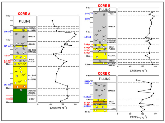
Figure 3.
La Fontanilla cove: variation with depth of the ∑ REE in sediments of Core A (inner zone) and Cores B and C (outer zone). Paleoenvironments and dating from [52,57,58]. Red: mean 14C calibrated age; blue: inferred age (geochemistry, pollen, etc.).
A high REE content (Σ REE = 140 mg kg−1) in the finer level of the shallow marine sediments from the MIS-1 transgression was found. Then, a tendency for an increase in the total REE contents is observed upwards, and the highest values occur in marsh deposits around 4 m depth (Σ REE = 175–183 mg kg−1). A significant decrease in the uppermost sediments (<1.9 kyr), corresponding to alluvial, marsh, and filling deposits, was found (Σ REE = 70–98 mg kg−1).
ii. Outer zone. A general tendency for a higher Σ REE is found in Cores B and C when compared to the inner zone. Core B, mainly corresponding to marsh sediments, presents high and uniform values (∑ REE = 134–176 mg kg−1). A higher variation is found in Core C, where a high REE content (Σ REE = 170 mg kg−1) in the finer level of the shallow marine sediments from the MIS-1 transgression was found. The uppermost sediments (freshwater pond) of Core B present higher values (Σ REE = 152–168 mg kg−1) than the filling materials of Core C (Σ REE = 91 mg kg−1) and Core A (inner zone; Σ REE = 70 mg kg−1).
High Σ REE values were found in fine marsh deposits in both zones dated around 1.9 kyr, particularly in the outer zone. These flooded marshes could have acted as REE repositories during the intensive exploitation of mineral deposits during the Roman period, which is in agreement with the high contents of As, Cr, Mn, and Zn, as well as Al, Fe, and S, found by [52,57,58]. Strong relative enrichment of the total REE concentrations in sediments collected in sites receiving drainage from acid sulfate soils in comparison to non-impacted sites in an estuary in Western Australia was also previously reported by [89].
Worth noting as well are the high REE values found in the marsh deposits of the three cores corresponding to the first prehistoric contamination (4.5 kyr), particularly in Core C when compared to the increase in the Roman period. The tendency of REE to concentrate in the topmost sediments, which can be related to the third and fourth contamination phases (1870–1960, and since 1990, respectively), was mainly found in the cores of the outer zone, in relation to recent mining activities (see Figure 3). Evidence of this mining period (1870–2001) was also found in this zone using the geochemical evolution of other metals [52,57,58], since REE are mainly derived from the extraction of ore deposits and industrial wastes. The Σ REE values found in this work in the outer zone are lower than those found in the gravity cores collected from the Tinto and Odiel estuaries by [83]; according to these authors, the high values, associated with high thorium concentrations, are caused by fertilizer industry wastes between 1968 and 1998, which used phosphorite as source material. However, in this work, similar and higher REE values are found lower in Cores B and C. Therefore, no clear evidence was found of the influence of phosphogypsum dumps on the Σ REE.
The uppermost meters of all cores are characterized by the transit to supratidal paleoenvironments and the disconnection between the tidal and fluvial inputs [52,57,58]. This subaerial exposure explains the reduction in the ∑REE values near the surface of these cores.
4.3.1. LaN/YbN Ratio
i. Inner zone. REE fractionation between the LREE and HREE (here measured by the LaN/YbN) is observed, with a general enrichment of the LREE relative to the HREE, particularly in the coarser sediments, which indicates a higher concentration of the LREE in coarser particles. The highest values were found in the MIS-1 flood coarser deposits (Figure 4, Core A).
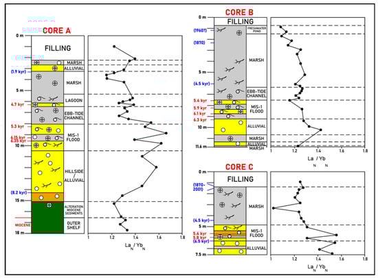
Figure 4.
La Fontanilla cove: variation with depth of the LaN/YbN ratio (normalized to PAAS) in sediments of Core A (inner zone) and Cores B and C (outer zone). Paleoenvironments and dating from [52,57,58]. Red: mean 14C calibrated age; blue: inferred age (geochemistry, pollen, etc.).
ii. Outer zone. An enrichment of the LREE relative to the HREE, particularly in the coarser sediments (around 10 m depth) in Core B, and around 6 m–7 m depth in Core C is observed; this tendency observed in the MIS-1 flood deposits in the outer zone appears to be similar to the one found in Core A.
A clear concentration of the LREE relative to the HREE in shallow marine sediments from the MIS-1 transgression in both zones occurs. This could be expected since LREE distribution in sediments could be related to the presence of sandy grains of feldspars and micas; this can also be partially explained by the change in water chemistry with increased salinity bringing about flocculation and settling out of colloids, as well as the higher particle reactivity of the LREE when compared to the HREE [90]. In fact, in water environments with a pH > 6, a preferential adsorption of the LREE on the particles is found, while the HREE preferably remain in solution [91], leading to an increase in the LREE relative to the HREE in sediments. Thus, a higher incorporation of the LREE when compared to the HREE in fine particles of the MIS-1 transgression sediments of the three cores could be expected.
4.3.2. LaN/SmN Ratio
i. Inner zone. REE fractionation between the LREE and MREE (here measured by LaN/SmN ratio) is observed, with a general enrichment of the MREE relative to the LREE (Figure 5). Miocene samples, including altered sediments, present a similar ratio (LaN/SmN = 0.86–0.89). Upwards, no clear tendency is observed; nevertheless, an enrichment in the LREE relative to the MREE is found in some coarser samples of the MIS-1 flood and in the more recent deposits (since 1.9 kyr), particularly in the marsh deposits.
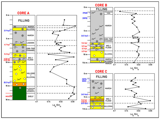
Figure 5.
La Fontanilla cove: variation with depth of the LaN/SmN ratio (normalized to PAAS) in sediments of Core A (inner zone) and Cores B and C (outer zone). Paleoenvironments and dating from [52,57,58]. Red: mean 14C calibrated age; blue: inferred age (geochemistry, pollen, etc.).
ii. Outer zone. A similar enrichment of the MREE relative to the LREE is found throughout Core B, and a higher variation is observed in Core C, with the lowest MREE enrichment in the MIS-1 flood deposits.
In this work, a general enrichment of the MREE relative to the LREE was found (LaN/SmN = 0.73–0.89). The enrichment of the MREE with respect to the LREE, and also to the HREE (see Figure 2), can be explained by preferential sorptive removal of the MREE via precipitation of poorly crystalline iron oxyhydroxides, typical of AMD-affected environments, which favor sediments that also preserve convex MREE patterns [39,92]. MREE enrichment, relative to the LREE and HREE, were already reported by [45] indicating acid-mixing processes between fluvial waters affected by AMD and seawater.
4.3.3. Eu Anomaly (Eu/Eu*)
i. Inner zone. Positive Eu anomalies through Core A occur, particularly in the marsh deposits down to circa 5000 kyr. The highest values were found in the ebb-tide channel deposits (Figure 6).
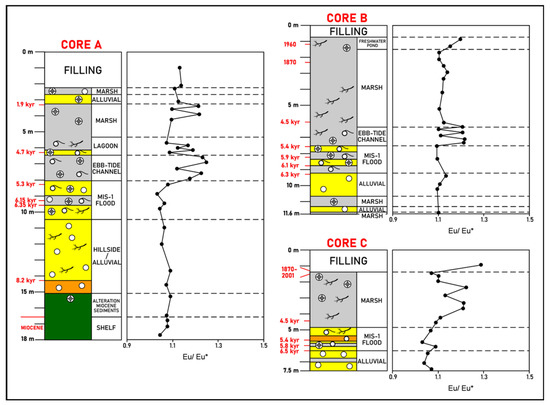
Figure 6.
La Fontanilla cove: variation with depth of the Eu anomaly (Eu/Eu* ratio, normalized to PAAS) in sediments of Core A (inner zone) and Cores B and C (outer zone). Paleoenvironments and dating from [52,57,68]. Red: mean 14C calibrated age; blue: inferred age (geochemistry, pollen, etc.).
ii. Outer zone. More significant positive Eu anomalies occur in the marsh deposits of the ebb-tide channel deposit of Core B and the marsh deposits of Core C.
Although not common in estuarine sediments, positive Eu anomalies in coarse sediments have been reported for other estuaries and associated with feldspar, particularly plagioclase, which has a positive Eu anomaly [93,94]. Although no mineralogical data were obtained for the studied sediments, fine particles of plagioclase could partially explain the positive Eu anomalies found. Nevertheless, the higher positive anomalies found in marsh deposits (Cores A and C) and in the ebb-tide channel deposits (Cores A and B) can also be due to the reduction of Eu(III) to Eu(II) and to the preferential removal of Eu3+ along with the other trivalent REE. In fact, according to [29], positive Eu anomalies in recent estuarine sediments were found in unique local conditions where the submarine groundwater discharge of reducing freshwaters, combined with organic matter decay and restricted saline oceanic water flow to these areas, may lead to the development of a strong localized salinity gradient. These unique conditions reduce the efficiency of sediment removal, leading to the consequent development of a positive Eu anomaly. Thus, the higher positive Eu anomalies found in marsh deposits of La Fontanilla cove may partially result from similar conditions described by [29].
4.3.4. Ce Anomaly (Ce/Ce*)
i. Inner zone. In general, small negative Ce anomalies through Core A (Ce/Ce* = 0.88-0.95) appear to occur (Figure 7).
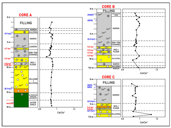
Figure 7.
La Fontanilla cove: variation with depth of the Ce anomaly (Ce/Ce* ratio, normalized to PAAS) in sediments of Core A (inner zone) and Cores B and C (outer zone). Paleoenvironments and dating from [52,57,58]. Red: mean 14C calibrated age; blue: inferred age (geochemistry, pollen, etc.).
ii. Outer zone. Small negative Ce anomalies appear to occur through Cores B and C.
It should be noted that some of the negative Ce anomalies found may be spurious given the potential for La anomalies in sea water to impact the calculation [9,11]. Moreover, about half of the samples fall in the range of 0.95–1.05, where they would be potentially unequivocal in meaning (not significant). To check whether the Ce anomalies are truly negative, the Pr/Pr* vs. Ce/Ce* is shown in Figure 8. Most of the samples of Core A are in field IIa, revealing no Ce anomaly and a positive La anomaly. However, samples of this core with a significant component of marine environments (littoral sandy deposits derived from the Bonares Sand Formation and deposits of the MIS-1 transgression) are in the field IIIb, indicating a negative Ce anomaly. In addition, most samples of the cores are in field I. An exception was found for sample C-15, which presents a negative La anomaly and no Ce anomaly (field IIb).
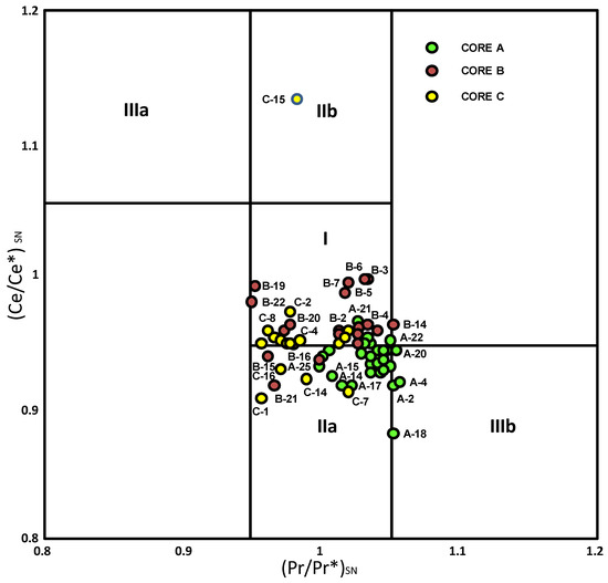
Figure 8.
Samples from La Fontanilla cove in a graph of (Ce/Ce*)SN vs. (Pr/Pr*)SN. Field I: neither CeSN nor LaSN anomaly; field Ila: positive Lass anomaly, no CeSN anomaly; field llb: negative LaSS anomaly, no CeSS anomaly; field Ilia: positive CeSN anomaly; field IIIb: negative CeSN anomaly. Modified from [9].
4.4. REE: Relation with Natural and Anthropogenic Inputs
The results obtained in this work from the sediments of the La Fontanilla cove (Tinto Estuary, SW Spain) show that the REE concentration distribution can be related to the depositional environment; nevertheless, the input of rare earths into sediments may have been modified by anthropogenic activities, such as mining/industrial inputs that led to favorable upward environmental conditions, i.e., to the dissolution of phases carrying REE (pyrite and other ore deposits). The old marshes, ebb-tide channels, lagoons, and freshwater ponds are constituted by clayey silts that present the highest REE contents, particularly around 4.5 kyr BP in the three cores and near the surface in Cores B and C. It should be noted that high contents of Cu, Pb, and As have also been detected in nearby cores studied by [95] and correlated with the first mining activities, as well as the recent mining and industrial wastes (1850–2000); in both polluted horizons, important percentages of pyrite (2–12%) were found.
The bioclastic sediments deposited during the MIS-1 transgression show great variability in grain sizes (clayey silts to bioclastic gravels) and REE contents, which can be partially explained by the presence of signficant quantities of shell fragments and valves of bivalves and gastropods. These shells are mostly composed of calcite and, to a lesser extent, aragonite [62].
The lower LREE/HREE in the finer sediments can be partially explained by the presence of heavy minerals, such as zircon and garnet, in the silt and clay fractions. REE tend not to be strongly complexed in solution, especially at low pH conditions [92], while at a circumneutral pH, carbonate complexes are often more abundant, with adsorption to particle surfaces becoming prevalent at mildly alkaline pH conditions [96]. A general enrichment of MREE, when compared to the other REE in the Tinto estuarine sediments, could be expected since this river crosses the Iberian Pyrite Belt. This can be partially explained by preferential release of the MREE, relative to the other REE, and most probably due to complexation to sulfite (SO32−) or another intermediate S-species during pyrite oxidation; the convex-upward REE pattern found in the acid sulfate soils developed on the salt marsh sediments of this estuary supports the possibility that iron oxyhydroxide minerals play an important role in MREE retention through adsorption and co-precipitation mechanisms. Thus, the normalized REE patterns of the estuarine sediments studied in this work that show convex curvatures in the MREE relative to LREE and HREE indicate acid-mixing processes between fluvial waters affected by AMD and seawater and precipitation of poorly crystalline mineral phases favoring the preservation of convex MREE patterns. While significant positive Eu anomalies were found in old ebb-tide channels and marsh deposits, most probably reflecting mineralogical composition and/or strong localized salinity gradient combined with organic matter degradation, no significant Ce anomalies were found. The small negative Ce anomaly found in a few cases may be spurious given the potential for La anomalies in sea water.
5. Conclusions
Rare earth elements’ concentrations and distribution patterns in sediment cores of the inner and outer zones of the La Fontanilla cove (Tinto estuary, SW Spain) display differences in their chemical contents and fractionations, reflecting their significant sensitivity to the environmental changes in this estuary. The total REE contents of these sediments are, in general, lower than those of the PAAS, particularly the HREE, which can be explained by the higher stability of heavy rare earths in aqueous complexes in this AMD environment. The total REE contents are higher in the finer sediments, which points to abundant mineral phases that are a better host for REE in the silt and clay fractions. The high total REE contents were also found to be related to the main episodes of mining activities (4500 yr BP) and industrial waste dumping (1850–2000).
The LREE/HREE ratio is mainly controlled by the grain size/mineralogy, which is higher in the coarser sediments. The LREE/MREE ratio is lower in marine environments. In the MIS-1 flood deposits, high values of the LREE, relative to the HREE and to the MREE, were also found, which indicates marine influence. Positive Eu/Eu* anomalies found in the marsh deposits and ebb-tide channels can be explained by a possible higher proportion of Eu carrier minerals (e.g., plagioclase) and/or indicate a local reduction in the conditions associated with an increase insalinity.
The REE distribution in the estuarine sediment cores of La Fontanilla cove, combined with sedimentary facies, prehistoric events, and historical events, significantly corroborates and improves the paleoenvironmental reconstruction. It should be noted that sedimentological characteristics of the deposits play a major role in the accumulation of REE and can mask the discharges caused by anthropogenic exploitation of pyrite ores.
Author Contributions
Conceptualization: M.I.P. and F.R.; methodology: all authors; software: J.M.M.; validation: M.I.P. and F.R.; formal analysis: all authors; investigation: all authors; resources: M.I.P., F.R. and J.R.V.; data curation: all authors; writing—original draft preparation: M.I.P. and F.R.; writing—review and editing: J.R.V., M.A. (Manuel Abad) and M.A. (Marta Arroyo); visualization: all authors; supervision: M.I.P. and F.R.; funding acquisition: M.I.P., F.R. and J.R.V. All authors have read and agreed to the published version of the manuscript.
Funding
Funds came from the Andalusian Government (groups RNM-238 and RNM-293), the town hall of Palos de la Frontera, and the FEDER 2014–2020 project UHU-1260298, which is a contribution to the Research Center in Historical, Cultural, and Natural Heritage (CIPHCN) of the University of Huelva. The C2TN/IST authors gratefully acknowledge the support of the FCT (the Portuguese Science and Technology Foundation) through the UIDB/04349/2020 project and the post-doctoral grant SFRH/BPD/114986/2016.
Data Availability Statement
Not Applicable.
Conflicts of Interest
The authors declare no conflict of interest.
References
- Turner, D.R.; Whitfield, M.; Dickson, A.G. The equilibrium speciation of dissolved components in freshwater and seawater at 25 °C and 1 atm pressure. Geochim. Cosmochim. Acta 1981, 45, 855–881. [Google Scholar] [CrossRef]
- Wood, S.A. The aqueous geochemistry of the rare-earth elements and yttrium: 1. Review of available low-temperature data for inorganic complexes and the inorganic REE speciation of natural waters. Chem. Geol. 1990, 82, 159–186. [Google Scholar] [CrossRef]
- Akagi, T. Rare earth element (REE) silicic acid complexes in seawater to explain the incorporation of REEs in opal and the “leftover” REEs in surface water: New interpretation of dissolved REE distribution profiles. Geochim. Cosmochim. Acta 2013, 113, 174–192. [Google Scholar] [CrossRef]
- Byrne, R.H.; Kim, K.H. Rare earth precipitation and coprecipitation behavior: The limiting role of PO43− on dissolved rare earth concentrations in seawater. Geochim. Cosmochim. Acta 1993, 57, 519–526. [Google Scholar] [CrossRef]
- Sholkovitz, E.R. The geochemistry of rare earth elements in the Amazon River estuary. Geochim. Cosmochim. Acta 1993, 57, 2181–2190. [Google Scholar] [CrossRef]
- McLennan, S.M. Rare earth elements in sedimentary rocks; influence of provenance and sedimentary processes. Rev. Mineral. Geochem. 1989, 21, 169–200. [Google Scholar]
- Toyoda, K.; Nakamura, Y.; Masuda, A. Rare earth elements of Pacific pelagic sediments. Geochim. Cosmochim. Acta 1990, 54, 1093–1103. [Google Scholar] [CrossRef]
- Sholkovitz, E.R.; Elderfield, H.; Szymczak, R.; Casey, K. Island weathering: River sources of rare earth elements to the Western Pacific Ocean. Mar. Chem. 1999, 68, 39–57. [Google Scholar] [CrossRef]
- Bau, M.; Dulski, P. Comparing yttrium and rare earths in hydrothermal fluids from the Mid-Atlantic Ridge: Implications for Y and REE behaviour during near-vent mixing and for the Y/Ho ratio of Proterozoic seawater. Chem. Geol. 1999, 155, 77–90. [Google Scholar] [CrossRef]
- Verplanck, P.L.; Nordstrom, D.K.; Taylor, H.E.; Kimball, B.A. Rare earth element partitioning between hydrous ferric oxides and acid mine water during iron oxidation. Appl. Geochem. 2004, 19, 1339–1354. [Google Scholar] [CrossRef]
- Bolhar, R.; Kamber, B.S.; Moorbath, S.; Fedo, C.M.; Whitehouse, M.J. Characterisation of early Archaean chemical sediments fy trace signatures. Earth Planet. Sci. Lett. 2004, 222, 43–60. [Google Scholar] [CrossRef]
- Benes, P.; Stamberg, K.; Vopalka, D.; Siroky, L.; Prochazkova, S. Kinetics of radioeuropium sorption on Gorelben sand from aqueous solutions and groundwater. J. Radioanal. Nucl. Chem. 2003, 256, 465–472. [Google Scholar] [CrossRef]
- Johannesson, K.H.; Tang, J.; Daniels, J.M.; Bounds, W.J.; Burdige, D.J. Rare earth element concentrations and speciation in organic-rich black waters of the Great Dismal Swamp, Virginia, USA. Chem. Geol. 2004, 209, 271–294. [Google Scholar] [CrossRef]
- Erel, Y.; Stolper, E.M. Modeling of rare-earth element partitioning between particles and solution in aquatic environments. Geochim. Cosmochim. Acta 1993, 57, 513–518. [Google Scholar] [CrossRef]
- Goldstein, S.L.; O′nions, R.K.; Hamilton, P.J. A Sm-Nd isotopic study of atmospheric dusts and particulates from major river systems. Earth Planet. Sci. Lett. 1984, 70, 221–236. [Google Scholar] [CrossRef]
- Tachikawa, K.; Athias, V.; Jeandel, C. Neodymium budget in the modern ocean and paleo-oceanographic implications. J. Geophys. Res. 2003, 108, 3254. [Google Scholar] [CrossRef]
- Elderfield, H.; Upstill-Goddard, R.; Sholkovitz, E.R. The rare earth elements in rivers, estuaries, and coastal seas and their significance to the composition of ocean waters. Geochim. Cosmochim. Acta 1990, 54, 971–991. [Google Scholar] [CrossRef]
- Sholkovitz, E.; Szymczak, R. The estuarine chemistry of rare earth elements: Comparison of the Amazon, Fly, Sepik and the Gulf of Papua systems. Earth Planet. Sci. Lett. 2000, 179, 299–309. [Google Scholar] [CrossRef]
- Lacan, F.; Jeandel, C. Tracing Papua New Guinea imprint on the central Equatorial Pacific Ocean using neodymium isotopic compositions and Rare Earth Element patterns. Earth Planet. Sci. Lett. 2001, 186, 497–512. [Google Scholar] [CrossRef]
- Johannesson, K.H.; Burdige, D.J. Balancing the global oceanic neodymium budget: Evaluating the role of groundwater. Earth Planet. Sci. Lett. 2007, 253, 129–142. [Google Scholar] [CrossRef]
- Rousseau, T.C.; Sonke, J.E.; Chmeleff, J.; Van Beek, P.; Souhaut, M.; Boaventura, G. Rapid neodymium release to marine waters from lithogenic sediments in the Amazon estuary. Nat. Commun. 2015, 6, 7592. [Google Scholar] [CrossRef] [PubMed]
- Du, J.; Haley, B.A.; Mix, A.C. Neodymium isotopes in authigenic phases, bottom waters and detrital sediments in the Gulf of Alaska and their implications for paleo-circulation reconstruction. Geochim. Cosmochim. Acta 2016, 193, 14–35. [Google Scholar] [CrossRef] [Green Version]
- Jeandel, C. Overview of the mechanisms that could explain the ‘Boundary Exchange at the land–ocean contact’. Phil. Trans. R. Soc. A 2016, 374, 20150287. [Google Scholar] [CrossRef] [PubMed] [Green Version]
- Welch, S.A.; Christy, A.G.; Isaacson, L.; Kirste, D. Mineralogical control of rare earth elements in acid sulfate soils. Geochim. Cosmochim. Acta 2009, 73, 44–64. [Google Scholar] [CrossRef]
- Hissler, C.; Hostache, R.; Iffly, J.F.; Pfister, L.; Stille, P. Anthropogenic rare earth element fluxes into floodplains: Coupling between geochemical monitoring and hydrodynamic sediment transport modelling. Compt. Rendus Geosci. 2015, 347, 294–303. [Google Scholar] [CrossRef]
- Kulaksız, S.; Bau, M. Contrasting behaviour of anthropogenic gadolinium and natural rare earth elements in estuaries and the gadolinium input into the North Sea. Earth Planet. Sci. Lett. 2007, 260, 361–371. [Google Scholar] [CrossRef]
- Kulaksız, S.; Bau, M. Anthropogenic dissolved and colloid/nanoparticle-bound samarium, lanthanum and gadolinium in the hine River and the impending destruction of the natural rare earth element distribution in rivers. Earth Planet. Sci. Lett. 2013, 362, 43–50. [Google Scholar] [CrossRef]
- Nordmyr, L.; Österholm, P.; Åström, M. Estuarine behaviour of metal loads leached from coastal lowland acid sulphate soils. Mar. Environ. Res. 2008, 66, 378–393. [Google Scholar] [CrossRef] [Green Version]
- Hannigan, R.; Dorval, E.; Jones, C. The rare earth element chemistry of estuarine surface sediments in the Chesapeake Bay. Chem. Geol. 2010, 272, 20–30. [Google Scholar] [CrossRef]
- Åström, M.E.; Österholm, P.; Gustafsson, J.P.; Nystrand, M.; Peltola, P.; Nordmyr, L.; Boman, A. Attenuation of rare earth elements in a boreal estuary. Geochim. Cosmochim. Acta 2012, 96, 105–119. [Google Scholar] [CrossRef]
- Johnston, S.G.; Morgan, B.; Burton, E.D. Legacy impacts of acid sulfate soil runoff on mangrove sediments: Reactive iron accumulation, altered sulfur cycling and trace metal enrichment. Chem. Geol. 2016, 427, 43–53. [Google Scholar] [CrossRef]
- Morgan, B.; Johnston, S.G.; Burton, E.D.; Hagan, R.E. Aciddic drainage drives anomalous rare earth element signatures in intertidal mangrove sediments. Sci. Total Environ. 2016, 573, 831–840. [Google Scholar] [CrossRef] [PubMed]
- Job, T.; Penny, D.; Morgan, B. Geochemical signatures of acidic drainage recorded in estuarine sediments after an extreme drought. Sci. Total Environ. 2020, 749, 141435. [Google Scholar] [CrossRef] [PubMed]
- Brito, P.; Caetano, M.; Martins, M.D.; Caçador, I. Effects of salt marsh plants on mobility and bioavailability of REE in estuarine sediments. Sci. Total Environ. 2021, 759, 144314. [Google Scholar] [CrossRef] [PubMed]
- Dellwiga, O.; Watermannb, F.; Brumsacka, H.-J.; Gerdesb, G. High-resolution Reconstruction of a Holocene Coastal Sequence (NW Germany) Using Inorganic Geochemical Data and Diatom Inventories. Estuar. Coast. Shelf Sci. 1999, 48, 617–633. [Google Scholar] [CrossRef]
- Thibault de Chanvalon, A.; Metzger, E.; Mouret, A.; Knoery, J.; Chiffoleau, J.-F.; Brach-Papa, C. Particles transformation in estuaries: Fe, Mn and REE signatures through the Loire Estuary. J. Sea Res. 2016, 118, 103–112. [Google Scholar] [CrossRef] [Green Version]
- Job, T.; Penny, D.; Hua, Q. Metal enrichment in estuarine sediments proximal to acid sulfate soils as a novel palaeodrought proxy. Sci. Total Environ. 2018, 612, 247–256. [Google Scholar] [CrossRef]
- Li, M.; Ouyang, T.; Zhu, Z.; Tian, C.; Peng, S.; Tang, Z.; Qiuc, Y.; Zhong, H.; Peng, X. Rare earth element fractionations of the northwestern South China Sea sediments, and their implications for East Asian monsoon reconstruction during the last 36 kyr. Quat. Int. 2019, 525, 16–24. [Google Scholar] [CrossRef]
- Johannesson, K.H.; Zhou, X.P. Origin of middle rare earth element enrichments in acid waters of a Canadian High Arctic lake. Geochim. Cosmochim. Acta 1999, 63, 153–165. [Google Scholar] [CrossRef]
- Borrego, J.; López-González, N.; Carro, B.; Lozano-Soria, O. Geochemistry of rare earth elements in Holocene sediments of an acidic estuary: Environmental markers (Tinto river estuary, Southwestern Spain). J. Geochem. Explor. 2005, 86, 119–129. [Google Scholar] [CrossRef]
- Gammons, C.H.; Wood, S.A.; Nimick, D.A. Diel behavior of rare earth elements in a mountain stream with acidic to neutral pH. Geochim. Cosmochim. Acta 2005, 69, 3747–3758. [Google Scholar] [CrossRef]
- Gammons, C.H.; Wood, S.A.; Pedrozo, F.; Varekamp, J.C.; Nelson, B.J.; Shope, C.L.; Baffico, G. Hydrogeochemistry and rare earth element behavior in a volcanically acidified watershed in Patagonia, Argentina. Chem. Geol. 2005, 222, 249–267. [Google Scholar] [CrossRef]
- Wood, S.A.; Gammons, C.H.; Parker, S.R. The behavior of rare earth elements in naturally and anthropogenically acidified waters. J. Alloy. Comp. 2006, 418, 161–165. [Google Scholar] [CrossRef]
- Pérez-López, R.; Delgado, J.; Nieto, J.M.; Márquez-García, B. Rare earth element geochemistry of sulphide weathering in the São Domingos mine area (Iberian Pyrite Belt): A proxy for fluid–rock interaction and ancient mining pollution. Chem. Geol. 2010, 276, 29–40. [Google Scholar] [CrossRef]
- Delgado, J.; Pérez-López, R.; Galván, L.; Nieto, J.M.; Boski, T. Enrichment of rare earth elements as environmental tracers of contamination by acid mine drainage in salt marshes: A new perspective. Mar. Pollut. Bull. 2012, 64, 1799–1808. [Google Scholar] [CrossRef]
- Grawunder, A.; Merten, D.; Büchel, G. Origin of middle rare earth element enrichment in acid mine drainage-impacted areas. Environ. Sci. Pollut. Res. 2014, 21, 6812–6823. [Google Scholar] [CrossRef]
- Prudêncio, M.I.; Valente, T.; Marques, R.; Sequeira Braga, M.A.; Pamplona, J. Geochemistry of rare earth elements in a passive treatment system built for acid mine drainage remediation. Chemosphere 2015, 138, 691–700. [Google Scholar] [CrossRef]
- Gomes, P.; Valente, T.; Geraldo, D.; Ribeiro, C. Photosynthetic pigments in acid mine drainage: Seasonal patterns and associations with stressful abiotic characteristics. Chemosphere 2020, 239, 124774. [Google Scholar] [CrossRef]
- Sarti, G.; Rossi, V.; Amorosi, A. Influence of Holocene stratigraphic architecture on ground surface settlements: A case study from the City of Pisa (Tuscany, Italy). Sediment. Geol. 2012, 281, 75–87. [Google Scholar] [CrossRef]
- Williams, J.; Dellapenna, T.; Louchouarn, P.; Lee, G. Historical reconstruction of anthropogenic mercury input from sedimentary records: Yeongsan Estuary, South Korea. Estuar. Coast. Shelf Sci. 2015, 167, 436–446. [Google Scholar] [CrossRef]
- Cheng, Z.; Jalon-Rójas, I.; Wang, X.H.; Liu, Y. Impacts of land reclamation on sediment transport and sedimentary environment in a macro-tidal estuary. Estuar. Coast. Shelf Sci. 2020, 242, 106861. [Google Scholar] [CrossRef]
- Arroyo, M.; Ruiz, F.; Campos, J.M.; Bermejo, J.; González-Regalado, M.L.; Rodríguez Vidal, J.; Cáceres, L.M.; Olías, M.; Abad, M.; Izquierdo, T.; et al. Where did Christopher Columbus start: The estuarine scenario of a historical date. Estuar. Coast. Shelf Sci. 2021, 250, 107162. [Google Scholar] [CrossRef]
- Martínez Cortizas, A.; López-Merino, L.; Bindler, R.; Mighall, T.; Kylander, M.E. Early atmospheric metal pollution provides evidence for Chalcolithic/Bronze Age mining and metallurgy in Southwestern Europe. Sci. Total Environ. 2016, 545, 398–406. [Google Scholar] [CrossRef] [PubMed] [Green Version]
- Elbaz-Poulichet, F.; Dupuy, C. Behaviour of rare earth elements at the freshwater-seawater interface of two acid mine rivers: The Tinto and Odiel (Andalucia, Spain). Appl. Geochem. 1999, 14, 1063–1072. [Google Scholar] [CrossRef]
- López-González, N.; Borrego, J.; Carro, B.; Grande, J.A.; De la Torre, M.L.; Valente, T. Rare-earth-element fractionation patterns in estuarine sediments as a consequence of acid mine drainage: A case study in SW Spain. Bol. Geol. Min. 2012, 123, 55–64. [Google Scholar]
- Mil-Homens, M.; Vale, C.; Naughton, F.; Brito, P.; Drago, T.; Anes, B.; Raimundo, J.; Schmidt, S.; Caetano, M. Footprint of roman and modern mining activities in a sediment core from the southwestern Iberian Atlantic shelf. Sci. Total Environ. 2016, 571, 1211–1221. [Google Scholar] [CrossRef] [PubMed]
- Arroyo, M.; Ruiz, F.; González-Regalado, M.L.; Rodríguez Vidal, J.; Cáceres, L.M.; Olías, M.; Campos, J.M.; Fernández, L.; Abad, M.; Izquierdo, T.; et al. Natural and anthropic pollution episodes during the Late Holocene evolution of the Tinto River estuary (SW Spain). Sci. Mar. 2021, 85, 113–123. [Google Scholar] [CrossRef]
- Rodríguez Vidal, J.; Cáceres, L.M.; Arroyo, M.; González-Regalado, M.L.; Gómez, P.; Ruiz, F. La construcción geológica de la bahía colombina. In La Recuperación Geoarqueológica del Puerto Histórico de Palos de la Frontera (s. XIV-XV); Campos, J.M., Ed.; Universidad de Huelva: Huelva, Spain, 2021; pp. 191–204. [Google Scholar]
- Civis, J.; Sierro, F.J.; González-Delgado, J.A.; Flores, J.A.; Andrés, I.; Porta, J.; Valle, M.F. El Neógeno marino de la provincial de Huelva: Antecedentes y definición de las unidades litoestratigráficas. In Paleontología del Neógeno de Huelva; Universidad de Salamanca: Salamanca, Spain, 1987; pp. 9–21. [Google Scholar]
- Mayoral, E.; Pendón, J.G. Icnofacies y sedimentación en zona costera. Plioceno Superior (?), litoral de Huelva. Acta Geol. Hisp. 1986, 21–22, 507–513. [Google Scholar]
- Pendón, J.G.; Rodríguez Vidal, J. Caracteres sedimentógicos y geomorfológicos del Alto Nivel Aluvial cuaternario en el litoral de Huelva. Acta Geol. Hisp. 1986, 21–22, 107–111. [Google Scholar]
- Borrego, J.; Morales, J.A.; Pendón, J.G. Holocene flling of an estuarine lagoon along the mesotidal coast of Huelva: The Piedras River mouth, southwestern Spain. J. Coast. Res. 1993, 9, 242–254. [Google Scholar]
- Davis, R., Jr.; Welty, A.; Borrego, J.; Morales, J.A.; Pendon, J.G.; Ryan, J.G. Rio Tinto estuary (Spain): 5000 years of pollution. Environ. Geol. 2000, 39, 1107–1116. [Google Scholar] [CrossRef]
- CEDEX (Centro de Estudios y Experimentación de Obras Públicas). Dinámica Litoral de la Flecha de El Rompido (Huelva); Ministerio de Obras Públicas: Madrid, Spain, 1991; p. 100. [Google Scholar]
- CEEPYC (Centro de Estudios y Experimentacion de Puertos y Costas ‘Ramon Iribarren’). Plan de Estudio de la Dinámica Litoral de la Provincia de Huelva; Informe Direccion General de Puertos y Costas: Madrid, Spain, 1979; p. 37. [Google Scholar]
- Cuena, G.J. Proyecto de Regeneración de las Playas de Isla Cristina. Informe del Servicio de Costas; Ministerio de Obras Publicas y Turismo: Madrid, Spain, 1991; p. 100. [Google Scholar]
- Galán, E.; González, I. Contribución de la mineralogía de arcillas a la interpretación de la evolución paleogeográfica del sector occidental de la cuenca del Guadalquivir. Estud. Geológicos 1993, 49, 261–275. [Google Scholar] [CrossRef]
- Ruiz, F.; Rodríguez-Ramírez, A.; Cáceres, L.M.; Rodríguez Vidal, J.; Carretero, M.I.; Abad, M.; Olías, M.; Pozo, M. Evidence of high-energy events in the geological record: Mid-Holocene evolution of the southwestern Doñana National Park (SW Spain). Palaeogeogr. Palaeoclimatol. Palaeoecol. 2005, 229, 212–229. [Google Scholar] [CrossRef]
- Galán, E.; Requena, A.; Fernández Caliani, J.C. Provenance and evolution of clay minerals in the Tinto river, SW Spain. Geol. Carphat. 1996, 5, 61–66. [Google Scholar]
- Fernández Caliani, J.C.; Ruiz, F.; Galán, E. Clay minerals and heavy metal distributions in the lower estuary of Huelva and adjacent Atlantic shelf, SW Spain. Sci. Total Environ. 1997, 198, 181–200. [Google Scholar] [CrossRef]
- Barba, C.; Fernández-Caliani, J.C.; Miras, A.; Galán, E. Mineralogía de los suelos y sedimentos actuales del estero Domingo Rubio (estuario de Huelva). Macla 2007, 7, 60. [Google Scholar]
- Requena, A.; Claus, F.L.; Fernandez-Caliani, J.C. Mineralogy and geochemical features of the recent sediments in the Odiel river (Huelva). Cuad. Lab. Xeol. De Laxe Coruña 1991, 16, 135–144. [Google Scholar]
- Tornos, F. La Geología y Metalogenia de la Faja Pirítica Ibérica. Macla 2008, 10, 13–23. [Google Scholar]
- Olías, M.; Cánovas, C.R.; Macías, F.; Basallote, M.D.; Nieto, J.M. The evolution of pollutant concentrations in a river severely affected by acid mine drainage: Río Tinto (SW Spain). Minerals 2020, 10, 598. [Google Scholar] [CrossRef]
- Nelson, C.H.; Lamothe, P.J. Heavy metal anomalies in the Tinto and Odiel River and estuary system, Spain. Estuaries 1993, 16, 496–511. [Google Scholar] [CrossRef]
- Ruiz, F. Trace metals in estuarine sediments from the southwestern Spanish coast. Mar. Poll. Bull. 2000, 42, 482–490. [Google Scholar] [CrossRef]
- R Core Team. R: A Language and Environment for Statistical Computing; R Foundation for Statistical Computing: Vienna, Austria, 2019. [Google Scholar]
- Gómez, G.; Ruiz, F.; Rodríguez Vidal, J.; González-Regalado, M.L.; Cáceres, L.M.; Gómez, P.; Abad, M.; Izquierdo, T.; Toscano, A.; Arroyo, M.; et al. Miocene-Late Quaternary environmental changes and mollucs as proxies of MIS-1 transgression in the Tinto-Odiel estuary, SW Spain. J. Iber. Geol. 2022, 48, 129–140. [Google Scholar] [CrossRef]
- Taylor, S.R.; McLennan, S.M. The Continental Crust: Its Composition and Evolution; Blackwell Scientific Publications: Oxford, UK, 1985; p. 312. [Google Scholar]
- Kramer, K.J.M.; Groenewoud, H.; Dorten, W.; Kramer, G.N.; Muntaun, H.; Quevauvillert, P.H. Certified reference materials for the quality control of rare earth element determinations in the environment. Trends Anal. Chem. 2002, 21, 762–773. [Google Scholar] [CrossRef]
- Yang, S.Y.; Jung, H.S.; Choi, M.S.; Li, C.X. The rare earth element compositions of the Changjiang (Yangtze) and Huanghe (Yellow) river sediments. Earth Planet. Sci. Lett. 2002, 201, 407–419. [Google Scholar] [CrossRef]
- Burbidge, C.I.; Trindade, M.J.; Dias, M.I.; Oosterbeek, L.; Scarre, C.; Rosina, P.; Cruz, A.; Cura, S.; Cura, P.; Caron, L.; et al. Luminescence dating and associated analyses in transition landscapes of the Alto Ribatejo, central Portugal. Quat. Geochron. 2014, 20, 65–67. [Google Scholar] [CrossRef]
- Marques, R.; Prudêncio, M.I.; Waerenborgh, J.C.; Rocha, F.; Ferreira da Silva, E.; Dias, M.I.; Madeira, J.; Vieira, B.J.C.; Marques, J.G. Geochemical fingerprints in topsoils of the volcanic Brava Island, Cape Verde. Catena 2016, 147, 522–535. [Google Scholar] [CrossRef]
- Borrego, J.; López-González, N.; Carro, B.; Lozano-Soria, O. Origin of the anomalies in light and middle REE in sediments of an estuary affected by phosphogypsum wastes (south-western Spain). Mar. Pollut. Bull. 2004, 49, 1045–1053. [Google Scholar] [CrossRef]
- Bohn, H.L.; Myerr, R.A.; O′Connor, G.A. Soil Chemistry; John Wiley & Sons: New Jersey, NJ, USA, 2002; p. 320. [Google Scholar]
- Paul, S.A.L.; Haeckel, M.; Bau, M.; Bajracharva, R.; Koschinsky, A. Small-scale heterogeneity of trace metals including rare earth elements and yttrium in deep-sea sediments and porewaters of the Peru Basin, southeastern equatorial Pacific. Biogeosciences 2019, 16, 4829–4849. [Google Scholar] [CrossRef] [Green Version]
- Ge, Q.; Xue, Z.G.; Chu, F. Rare Earth Element distributions in continental shelf sediment, Northern South China Sea. Water 2020, 12, 3540. [Google Scholar] [CrossRef]
- Alhassan, A.B.; Aljahdali, M.O. Fractionation and Distribution of Rare Earth Elements in Marine Sediment and Bioavailability in Avicennia marina in Central Red Sea Mangrove Ecosystems. Plants 2021, 10, 1233. [Google Scholar] [CrossRef]
- Morgan, B.; Rate, A.W.; Burton, E.D.; Smirk, M.N. Enrichment and fractionation of rare earth elements in FeS- and organic-rich estuarine sediments receiving acid sulfate soil drainage. Chem. Geol. 2012, 308, 60–73. [Google Scholar] [CrossRef]
- Edzwald, J.K.; Upchurch, J.B.; O′Melia, C.R. Coagulation in estuaries. Environ. Sci. Technol. 1974, 8, 58–63. [Google Scholar] [CrossRef]
- Sholkovitz, E. Chemical evolution of Rare Earth Elements: Fractionation between colloidal and solution phases of filtered river water. Earth Planet. Sci. Lett. 1992, 114, 77–84. [Google Scholar] [CrossRef]
- Bau, M. Scavenging of disolved yttrium and rare earth elements by precipitating iron oxyhydroxide experimental evidence for Ce-oxidation, Y-Jo fractionation and lanthanide tetrad effect. Geochim. Cosmochim. Acta 1999, 63, 67–77. [Google Scholar] [CrossRef]
- Ramesh, R.; Ramanathan, A.; Ramesh, S.; Purvaja, R.; Subramanian, V. Distribution of rare earth elements and heavy metals in the surficial sediments of the Himalayan river syste. Geochem. J. 2000, 34, 295–319. [Google Scholar] [CrossRef]
- Brito, P.; Prego, R.; Mil-Homens, M.; Caçador, I.; Cartano, M. Sources and distribution of yttrium and rare elements in surface sediments from Tagus estuary, Portugal. Sci. Total Environ. 2018, 621, 317–325. [Google Scholar] [CrossRef] [PubMed]
- Leblanc, M.; Morales, J.A.; Borrego, J.; Elbaz-Poulichet, F. 4500-year-old pollution in southwestern Spain: Long-term implications for modern mining pollution. Econ. Geol. 2000, 95, 655–662. [Google Scholar]
- Liu, H.; Pourret, O.; Guo, H.; Bonhoure, J. Rare earth elements sorption to iron oxyhydroxide; Model development and application to groundwater. Appl. Geochem. 2017, 87, 158–166. [Google Scholar] [CrossRef]
Publisher’s Note: MDPI stays neutral with regard to jurisdictional claims in published maps and institutional affiliations. |
© 2022 by the authors. Licensee MDPI, Basel, Switzerland. This article is an open access article distributed under the terms and conditions of the Creative Commons Attribution (CC BY) license (https://creativecommons.org/licenses/by/4.0/).