The Influence of Particle Size on Sliding Wear of a Convex Pattern Surface

Abstract

Sliding wear of bulk handling equipment (e.g., shovel bucket, mill and transfer chute) can be dramatically reduced by using a convex pattern surface compared to a flat surface, by adjusting the flow behavior of particles moving along the convex pattern surface. To study the effect of particle size relative to the dimensions of the convex pattern surface, a coarse graining technique is applied. Comparisons of bulk flow and wear behavior between the convex pattern and flat surfaces illustrate the two-sided effect of the convex pattern surface on sliding wear. The bulk flow behavior indicates that the particle size has a minor effect on the velocity and angular velocity of particles for the flat surface, while it has a significant effect on those of the convex pattern surface. The wear results show that the particle size has negligible influence on the sliding wear of a flat surface and a linear relationship with the sliding wear of the convex pattern surface. The convex pattern surface can reduce the sliding wear through influencing the flow behavior of the bulk material when the equivalent radius of the convex is larger than $r_{50}$ of particles. This research reveals the relationship between the dimensions of the convex pattern and the particle size on the sliding wear caused by the interaction between bulk material and bulk handling equipment. The relationship should be carefully considered for the applications of the convex pattern surface to bulk handling equipment.

1. Introduction

The handling of bulk solids plays an important role in a variety of industries, such as the mining, agricultural, chemical, and pharmacological industries [1]. For the mining industry, the process of transferring bulk solids leads to surface wear of shovel buckets [2]. The vertical stirred mills are applied widely in mineral industries and the liner wear plays a significant role in the maintenance and operational costs [3]. Severe wear has been found in several locations on bulk handling equipment, for example, silo walls and bottom sections of the transfer chute [4]. For transfer chutes, studies show that approximately 82% of the energy losses are attributed to the bulk material sliding along the bottom of the chute, and 9% of the losses are due to sliding against the side walls [5]. To reduce the wear caused by the interaction between bulk material (e.g., soil and iron ore) and equipment surface (e.g., shovel bucket and transfer chute), scientists have proposed biological wear-resistant surfaces inspired by the contacts between biological surfaces and the corresponding living environments. Inspired by the bionic design method, a convex pattern surface is introduced [6] and optimized [7] to reduce the sliding wear of the surfaces of bulk solids handing equipment by using a discrete element method (DEM). Many works [8,9,10,11,12,13,14,15,16] have been completed on the investigation of sliding wear caused by the bulk material based on the DEM method, while other studies [9,11,12,13,14,16] whilwhile seldom focused on the influence of particle size on sliding wear. Although the previous studies have shown that the convex pattern surface can significantly reduce sliding wear compared with the flat surface, the effect of particle size is still unknown. The effect of particle size is crucial as the bulk handling equipment transfers various materials with different particle sizes. To bridge this gap, the study aims at the effect of particle size on the sliding wear of the bionic surface.

Based on the previous study [7], to investigate the influence of particle size on the sliding wear of the convex pattern surface, a particle scaling technique is applied. Various scaling techniques can be used for DEM, such as exact scaling [17,18], scalping [19], coarse graining [20], hybrid particle-geometric approach [21], and multi-level coarse graining [22].

The exact scaling aims at setting a numerical model that can reproduce the physical phenomena exactly. Three similarity principles, namely geometric, mechanical, and dynamic, must be satisfied to meet exact scaling [18]. The system parameters, for instance the acceleration of gravity, can be determined by the basic quantities, for instance length L, density $\rho$, and time T. As the domain and the particle size scale up together, so the upscaled system has the same number of particles and the same computational costs. For example, the particles and equipment are scaled to experimentally investigate excavating motion characteristic for grabs, reclaimers, and bulldozers [23]. For the scalping technique, the real PSD is scalped at a specific particle diameter, and only the larger particle size fractions are considered in the simulation [24]. For example, the finer fractions of the particles are omitted by replacing them with larger particles.

Another approach is called coarse graining or non-exact scaling [24] and the objective of coarse graining is to reduce computational time by replacing physical particles with representative parcels [20], so upscaled particles can be treated as pseudo-particles [18] or “meso” particles [25]. The key limitation of the particle upscaling factor is the precise representation of a process and therefore difficult to determine in general [24]. For example, the coarse graining technique was used to demonstrate the effect of particle upscaling on material equipment interactions for tool penetration and sliding regimes, and scaling factors 3 and 5 are determined for Hertz-Mindlin with rolling model C and with restricted particle rolling [26]. Another example indicates that an angle of repose test using a lifting cylinder discovers that the repose angle is invariant with respect to the dimensions of the lifting cylinder and the particle size [24]. A confined compression and unconfined loading process revealed that the contact stiffness for loading and unloading scales linearly with particle size and the adhesive force scales very well with the square of the particle size [27]. In addition, coarse graining can also be applied to investigate silo flow [28], granular mixing [29], and the powder die-filling system [30].

The hybrid particle-geometric scaling approach was proposed to scale DEM simulations by isolating the effects of varying particle size and geometric dimensions on bulk properties [21]. This approach successfully extends the coarse graining technique to incorporate elastoplastic behavior and cohesive forces [21]. Multi-level coarse graining allows the couple of multiple coarse grain levels to overcome the errors caused by the upscaling procedure of the conventional DEM coarse grain model [22], but this is difficult to implement.

Although the scaling approach is widely applied to the granular systems mentioned above, the application of the approach on sliding wear caused by bulk material with different sizes is still unstudied. The coarse graining technique is chosen in this research as it is suitable for non-cohesive and free-flowing material. The aim of this research is to investigate the influence of particle size on the sliding wear of the convex pattern surface based on the coarse graining approach. The structure of the article is outlined below. In Section 2, the effect of particle size on the contact behavior among particles and wear behavior for single particle-surface interactions is investigated through the coarse graining technique. Section 3 builds a simulation setup to conduct the sliding wear and Section 4 clarifies the methods used to analyze the simulation results. The comparisons of the simulation results between the convex pattern surface and a flat surface are elaborated on from three aspects in Section 5. Section 6 draws four main conclusions.

2. Particle Upscaling Theory

2.1. Contact Model

In the coarse graining method, the original particles with radius R are replaced by larger particles with radius R^’. To guarantee the identical physical behavior, the coarse-scaled system should keep the consistent energy density and energy density evolution with the original system. Therefore, the gravitational acceleration g, particle density $\rho$, and velocity v should be kept constant to retain the energy conservative. The motion of each particle follows Newton’s equations and the normal and tangential forces of spring-damping model in EDEM [31] can be denoted as Equations (1) and (2):

$${\mathrm{F}}_n=k_n{\delta }_n^{1/2}-{\gamma }_n\dot{{\delta }_n}$$

(1)

$${\mathrm{F}}_t=k_t{\delta }_t-{\gamma }_t\dot{{\delta }_t}$$

(2)

where $k_{n,t}$, ${\gamma }_{n,t}$, and ${\delta }_{n,t}$ are stiffness coefficients, damping coefficients, and overlap, respectively, and the subscripts $n$ and $t$ denote normal and tangential direction, respectively.

Applying the Hertzian and non-linear damping [22,32] theories, the stiffness and damping coefficients are formulated as in Equation (3):

$$\begin{array}{c}{k}_n=\frac{4}{3}{E}^{*}\sqrt{R^{*}{\delta }_n}\\ {\gamma }_n=-\beta \sqrt{5m^{*}{k}_n}\\ k_t=8G^{*}\sqrt{R^{*}{\delta }_n}\\ {\gamma }_t=-\beta \sqrt{\frac{10}{3}{m}^{*}{k}_t}\\ \beta =\frac{\ln \left(e\right)}{\sqrt{l{n}^2\left(e\right) + {\pi }^2}}\end{array}$$

(3)

Where $E^{*}$,$G^{*}$,$R^{*}$, and $m^{*}$ are the equivalent Young’s modulus, shear modulus, particle radius, and mass, respectively, and $e$ is the coefficient of restitution, which is defined as the ratio of the relative particle velocity before and after the collision. Furthermore, a rolling model A, which depends on the relative rotational velocity of two particles, is applied to the motion of particles [33].

Assuming two particles with radii $R_i$, $R_j$ contacting each other, the equivalent radius $R^{*}$ can be identified at Equation (4):

$$R^{*}=\frac{R_i{R}_j}{R_i+R_j}=\frac{\alpha R_i}{1+\alpha }$$

(4)

where $\alpha =R_j/R_i$. Similarly, the equivalent mass is shown in Equation (5):

$$m^{*}=\frac{m_i{m}_j}{m_i+m_j}=\rho \frac{4\pi R_i^3{\alpha }^3}{3\left(1+{\alpha }^3\right)}$$

(5)

To substitute Equation (1) with the dimensionless mass $m^{*\prime }=m^{*}/\rho R_i^3$, overlap ${\delta }_n^{\prime }={\delta }_n/R_i$, velocity ${\dot{\delta }}_n^{\prime }=\dot{{\delta }_n}/v_0$, and acceleration $\ddot{{\delta }_n^{\prime }}=\ddot{{\delta }_n}{R}_i/v_0^2$ with the reference velocity $v_0=\sqrt{E^{*}/\rho }$, the Equation (1) can be denoted as Equation (6):

$$m^{*\prime }\ddot{{\delta }_n^{\prime }}=\frac{k_n{\delta }_n^{\prime }}{R_i{E}^{*}}-\frac{{\gamma }_n\dot{{\delta }_n^{\prime }}}{R_i^2\sqrt{\rho E^{*}}}$$

(6)

Therefore, the scaling is based on dimensionless normal overlap for the translational motion of a particle [20] and the dimensional analysis of Equations (1) and (2) yield the invariant parameters shown in Equation (7):

$$\begin{array}{c}\prod 1=\frac{R_j}{R_i}\\ \prod 2=\frac{k_{n\left(t\right)}}{R_i{E}^{*}}\\ \prod 3=\frac{{\gamma }_{n\left(t\right)}}{R_i^2\sqrt{\rho E^{*}}}\end{array}$$

(7)

where $\prod 1$ is related to geometric similarity and indicates that the particle needs to be scaled with the constant ratio and $\prod 2$ and $\prod 3$ require that the $k_{n\left(t\right)}/R_i$ and ${\gamma }_{n\left(t\right)}/R_i^2$ be constant, since the velocity and density are scale-invariant.

For the stiffness coefficients in Equation (3), it is observed that the stiffness is scaled with the scaling factor $s$, as $s=R_{CG}/R_o$. $R_{CG}$ and $R_o$ are the coarse grained and original particle radii. The damping coefficient is scaled with $s^2$ as the $m^{*}$ and $k_n$ are scaled with $s^3$ and $s$, respectively. Therefore, the Hertz-Mindlin model is termed scale-invariant. Moreover, as the coarse grain has the same rotational energy as the original particles [26], the rolling model remains unchanged.

2.2. Archard Wear Model

Archard wear model [34] is applied to calculate the wear volume caused by the sliding of particles. This wear model has been used widely for bulk handling process, such as the prediction of the wear of mill lifters [35] and local failure prediction of abrasive wear on tipper bodies [36]. Equation (8) shows the generalized equation to calculate sliding wear volume:

$$W_v=k\frac{F_n}{H_s}{l}_s$$

(8)

where $W_v\left({\mathrm{mm}}^3\right)$ is the wear volume, $H_s\left({\mathrm{Nmm}}^{-2}\right)$ is the hardness of the surface, $k$ is a dimensionless wear coefficient, $F_n\left(N\right)$ is the normal force applied to an equipment surface, and $l_s\left(\mathrm{mm}\right)$ is the sliding distance. Obviously, particle size has no influence on the sliding wear model, so the Archard wear model is scale-invariant to particle size.

3. Verification of Model Scale Invariance

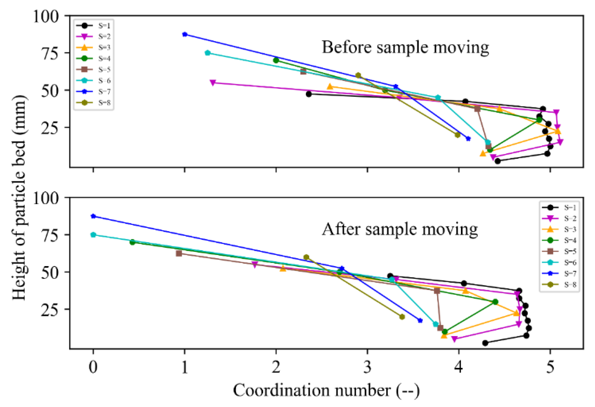
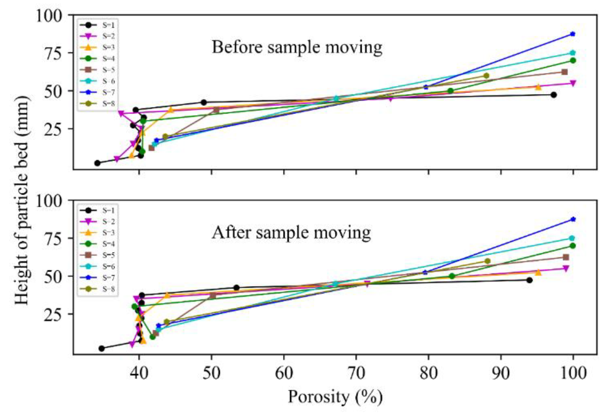
3.1. Packing

In order to guarantee similar contact behavior between particles, the microstructure (e.g., particle density and coordination number) and macrostructure (e.g., bulk density and porosity) should be invariant to particle size. The coordination number and porosity are used to investigate the contact behavior through a packing process [37]. In this process, the particle size is scaled up corresponding to the scale factor, while the dimensions of the simulation domain remain unchanged.

River gravel is used in this research, and this material is classified as dry, non-cohesive, and free-flowing. A sample of the river gravel is shown in Figure 1, and particle size distributions from scaling factor 1 to 8 are shown in Figure 2.

Table 1. General DEM parameters.

Categories	Parameters	Values
Contact model	-	Hertz-Mindlin (no slip)
Rolling friction model	-	Type A
River sand	Particle density $(\mathrm{kg}/{\mathrm{m}}^3)$	2460
	Poisson ratio $\mathsf{\vartheta }$ (-)	0.24
	Shear modulus $\mathrm{G} \left(\mathrm{GPa}\right)$	0.07
Steel	Density $(\mathrm{kg}/{\mathrm{m}}^3)$	7932
	Poisson ratio $\mathsf{\vartheta }$ (-)	0.3
	Shear modulus $\mathrm{G} \left(\mathrm{GPa}\right)$	78
Particle-particle	Coefficient of restitution (-)	0.45
	Coefficient of static friction (-)	0.21
	Coefficient of rolling friction (-)	0.4
Particle-steel	Coefficient of restitution (-)	0.6
	Coefficient of static friction (-)	0.38
	Coefficient of rolling friction (-)	0.3
Time step	$\mathsf{\Delta }\mathrm{t} \left(\mathrm{s}\right)$	$5\times {10}^{-6}$
Gravitational acceleration	$\mathrm{m}/{\mathrm{s}}^2$	9.81

lists the calibrated parameters for the DEM model and the parameters refer to the previous work [7].

A container, as shown in Figure 3, with length and width of 300 mm was filled with particles to a height of 300 mm, and periodic boundaries in length and width direction were used to avoid a wall effect. The particles moving out from one side re-entered into the wall at another side and the boundaries are represented by the dashed line shown in Figure 3. A bin group with the dimensions of $250 \mathrm{mm}\times 250\times 300 \mathrm{mm}$ was set in the container, and the depth of each bin is four times of $d_{50}$ (particle diameter corresponding to 50% of cumulative mass). After being filled, the container was vibrated for 4 s in the y-direction following a formula shown in Equation (9) and kept still for 5 s:

$$y=Asin\left(\omega t\right)$$

(9)

where $A=0.1d_{50}$ and $\omega =200{ \mathrm{rads}}^{-1}$.

The coordination number and porosity were investigated under the loose and dense packing states. Figure 4 shows the coordination number and the difference between the loose and dense packing. As shown in Figure 4a, the bottom and second bins showed the lowest and highest coordination number because of the wall effect and the particle consolidation. The coordination number decreased slowly from the third bin and dramatically at the last two bins. In order to eliminate the influence of wall effect and bulk consolidation, the bottom and top bins were excluded in the following analyses. It can be seen from Figure 4a that before vibration, the coordination number for all scaling factors was higher than 5 and lower than 5.6. After the vibration, as shown in Figure 4b, the coordination number was increased by 0.1 to 0.4.

For the porosity, if the center of a particle is located inside a bin, the whole volume of the particle was computed inside the bin. Figure 5 shows the opposite trend to the coordination number. Before vibration, as shown in Figure 5a, it was lower for lower scaling factors and increased from the second bin to the top bin for each scaling factor. After the vibration from Figure 5b, the porosity was decreased by less than 4%. The coordination number and porosity indicated that the vibration has an obvious influence on the contact among particles, because vibration induced compressed and relaxed effects which were competing with each other on the particles [38].

For both before and after vibration, the coordination number and porosity had a more obvious fluctuation for a scaling factor higher than 4 compared with those of a scaling factor lower than 4. The reason is that the dimensions of each bin were only changed in the depth direction, leading to the reduction of the particle numbers in each bin with the increase of the scaling factor, and therefore, the number of particles influenced the particle contact behavior.

3.2. Pin-on-Disc Test

The pin-on-disc test, as shown in Figure 6, was used to investigate the influence of particle size on sliding wear. A disc with a radius of 100 mm was meshed with 1 mm triangular meshes using ANSYS Workbench software package (18.2, ANSYS, Canonsburg, PA, USA) [39]. A particle body force (PBF) was applied to the particle to generate the normal force by implementing a EDEM API model [31]. To avoid particle movement, a cylindrical holder was located on the disc with a distance of 80 mm from the center of the disc. To eliminate the influence of the gravitational force of the particle, the masses of particles with different radii were kept constant by adjusting the particle density. A rotational velocity of 180 deg/s around the central axis was applied to the disc, and the total sliding wear volume was calculated after one round.

The simulation results were compared with the theoretical results, which were considered as a reference under the normal force of 1N, as shown in Figure 7. The result shows that the simulation results were comparable with the analytical result with a discrepancy less than 0.6%. It indicates that particle size had an ignorable effect on sliding wear, and the result was consistent with a previous study [40].

4. Simulation Setup and Analysis Procedures

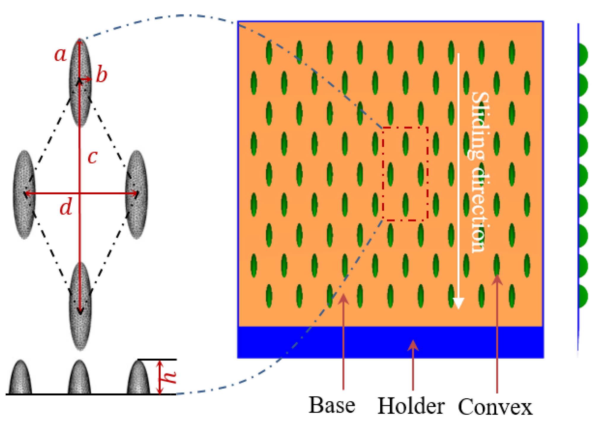
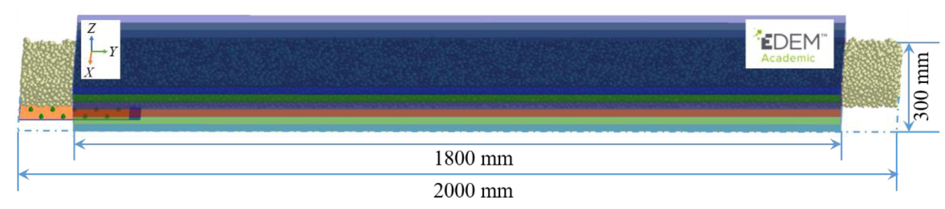
4.1. Simulation Setup

Figure 8 illustrates a surface of a convex pattern that can be described by five parameters: major and minor radii $a$ and $b$; vertical and horizontal distances $c$ and $d$; height of the convex $h$. An optimal sample with dimensions of these five parameters of 4 mm, 8 mm, 40 mm, 60 mm and 6 mm, respectively, was investigated [7]. To ensure that sliding wear occurs only on the top surface, the sample was covered by a holder with dimensions of $200 \mathrm{mm}\times 200 \mathrm{mm}$. Moreover, the sample was meshed by triangular meshes of 1 mm in size.

Figure 9 shows a particle bed clipped in the sample moving direction with 40 kg of particles, and the dimensions of the bed were $2000 \mathrm{mm}\times 300 \mathrm{mm}$ (length and width). The sample was located at the left central side of the particle bed and moved in the y-direction with a velocity of $2 \mathrm{m}/\mathrm{s}$. To eliminate the wall effect, a periodic boundary condition was applied to the width direction. A bin group, which was used to investigate the contact behavior among particles, was created at the particle bed. The length and width of each bin were 1800 mm and 300 mm, respectively.

Figure 10 illustrates the moving bins used to investigate the bulk flow behavior. The bins, which were ordered from bottom to the top of the particle bed with the same dimensions of the sample, were attached to and move with the sample. The depth of the bin was related to scaling factor, as listed in

Table 2. Sizes and layers of the bins.

Scaling Factor	${\mathit{d}}_{50} \left(\mathbf{mm}\right)$	Bin Group Height (mm)	Layers of Bins
1	2.65	60	12
2	5.3	60	6
3	7.95	60	4
4	10.6	80	4
5	13.25	75	3
6	15.9	90	3
7	18.55	105	3
8	21.2	80	2

. The ratio of bin depth to scaling factor is set as 5 to guarantee the layer of particles for different scaling factors constant. As the particle flow behaves differently, the layers of bins for different scaling factors varied.

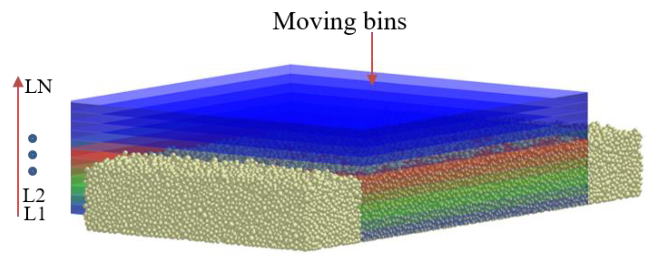
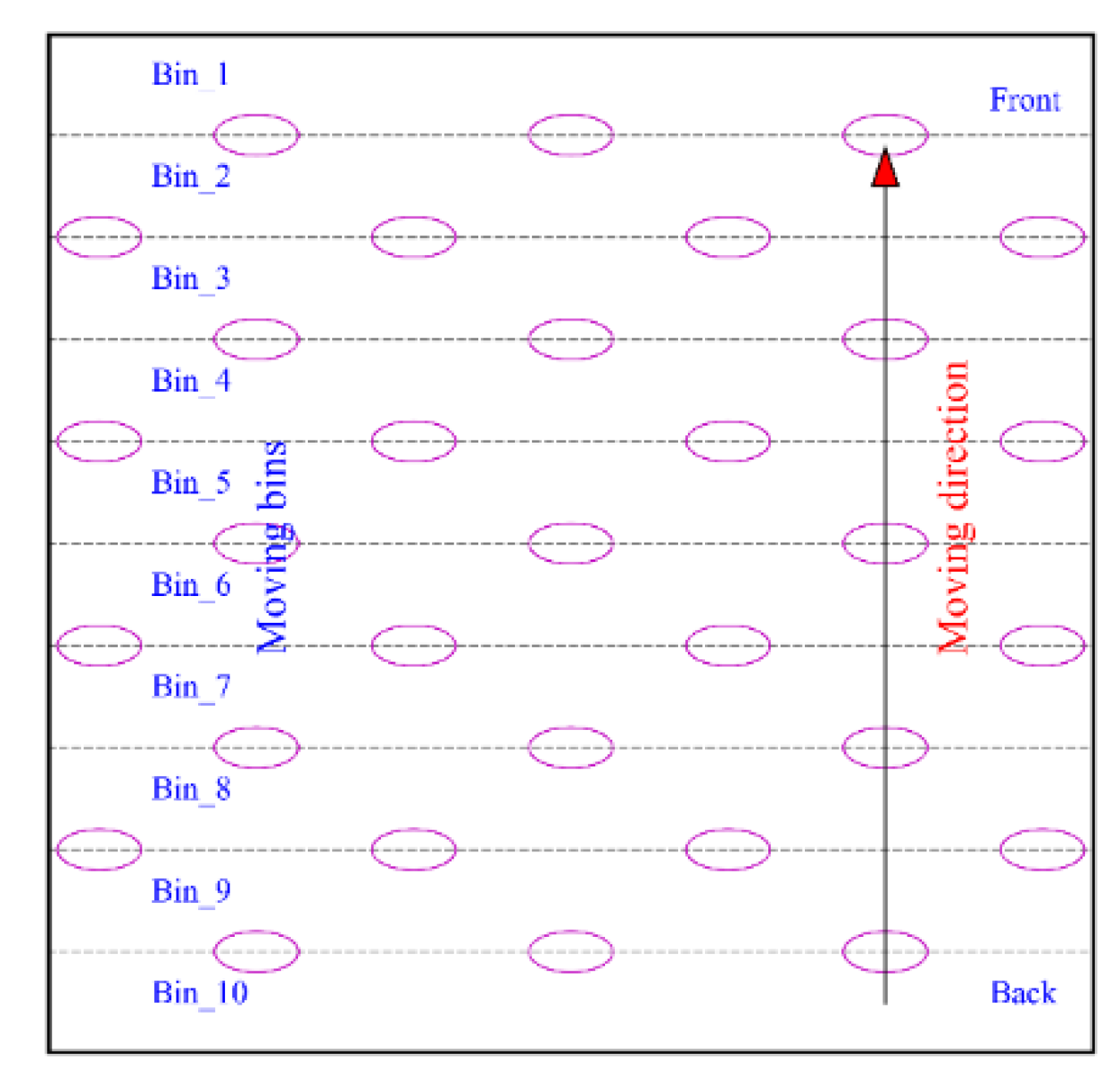
4.2. Analysis Procedures

The analysis of the wear results is related to the steady state of the simulation setup. Therefore, the stability of the simulation setup is first evaluated including two aspects, i.e., a stable state and dynamic state. The stable state focuses on the bulk contact behavior when the sample is located at a specific position. The dynamic state is evaluated by two criteria, the relative velocity of the bulk material and the relative wear rate of the sample.

For the relative velocity of bulk material, it should be noted that only the particles in the moving bins (see Figure 10) with the original particle bed height are considered. The relative velocity $\eta$ is defined as Equation (10):

$$\eta =\frac{\overline{v_{p,y}}}{v_s}\times 100\%$$

(10)

where η is relative velocity, $\overline{v_{p,y} }\left({\mathrm{mm} \mathrm{s}}^{-1}\right)$ is the averaged particle velocity in sample moving direction, and $v_s \left({\mathrm{mm} \mathrm{s}}^{-1}\right)$ is the velocity of the sample.

The wear rate $\phi$ is denoted by Equation (11):

$$\phi =\frac{W_{v,s}-W_{v,s-\mathsf{\Delta }s}}{\mathsf{\Delta }l}$$

(11)

where $\phi \left({\mathrm{mm}}^2\right)$ is the wear rate, $\mathsf{\Delta }l \left(\mathrm{mm}\right)$ is the displacement increment of the sample, and $W_{v,s}-W_{v,s-\mathsf{\Delta }s} \left(\mathrm{mm}\right)$ is the wear volume increment.

The relative wear rate ${\phi }_R$ is used to evaluate the stability of the sliding wear process, which is denoted by Equation (12):

$${\phi }_R=\frac{\phi }{\max \left(\phi \right)}\times 100\%$$

(12)

where ${\phi }_R$ is the relative wear rate and $\max \left(\phi \right) \left({\mathrm{mm}}^2\right)$ is the maximum wear rate of all simulations. For the convex pattern sample, Equations (11) and (12) can be used to calculate the wear results of the base and convex pattern, respectively.

After the analysis of the stability of the simulation setup, the sliding wear result was investigated. A relative wear $\gamma$ was used to compare the wear result, as denoted by Equation (13):

$$\gamma =\frac{W_v}{W_{v,flat,s=1}}\times 100\%$$

(13)

where $\gamma$ is the relative wear and $W_v \left({\mathrm{mm}}^3\right)$ and $W_{v,flat,s=1} \left({\mathrm{mm}}^3\right)$ are the wear volumes of the sample and a flat surface, respectively, caused by the original particles.

5. Results

This part compares the sliding wear and bulk flow behavior between the convex pattern and flat surfaces at a steady state, including the steady-state evaluation, bulk flow, and sliding wear behavior.

5.1. Steady-State Evaluation

5.1.1. Contact Behavior

The contact behavior of the particles was consistent with the packing, including the coordination number and porosity, and the particle bed with a flat surface was taken as a reference. Figure 11 shows that the coordination number of the original particle bed was higher than 5 for the scaling factor 1 to 5 and less than 5 for the others. After the travel of the sample, the coordination number for all scaling factor was lower than that of the original particle bed. Porosity showed an opposite trend to the coordination number, as shown in Figure 12, and increased with an increasing scaling factor. On the basis of both the coordination number and porosity, it can be seen that the flat surface can influence the contact behavior among particles and force the particle bed to switch from a relative dense state to a loose state.

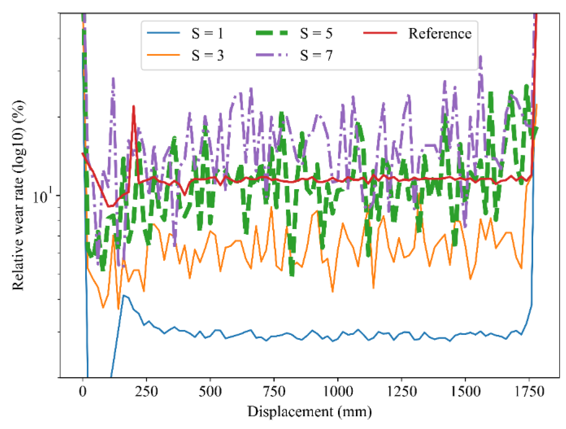
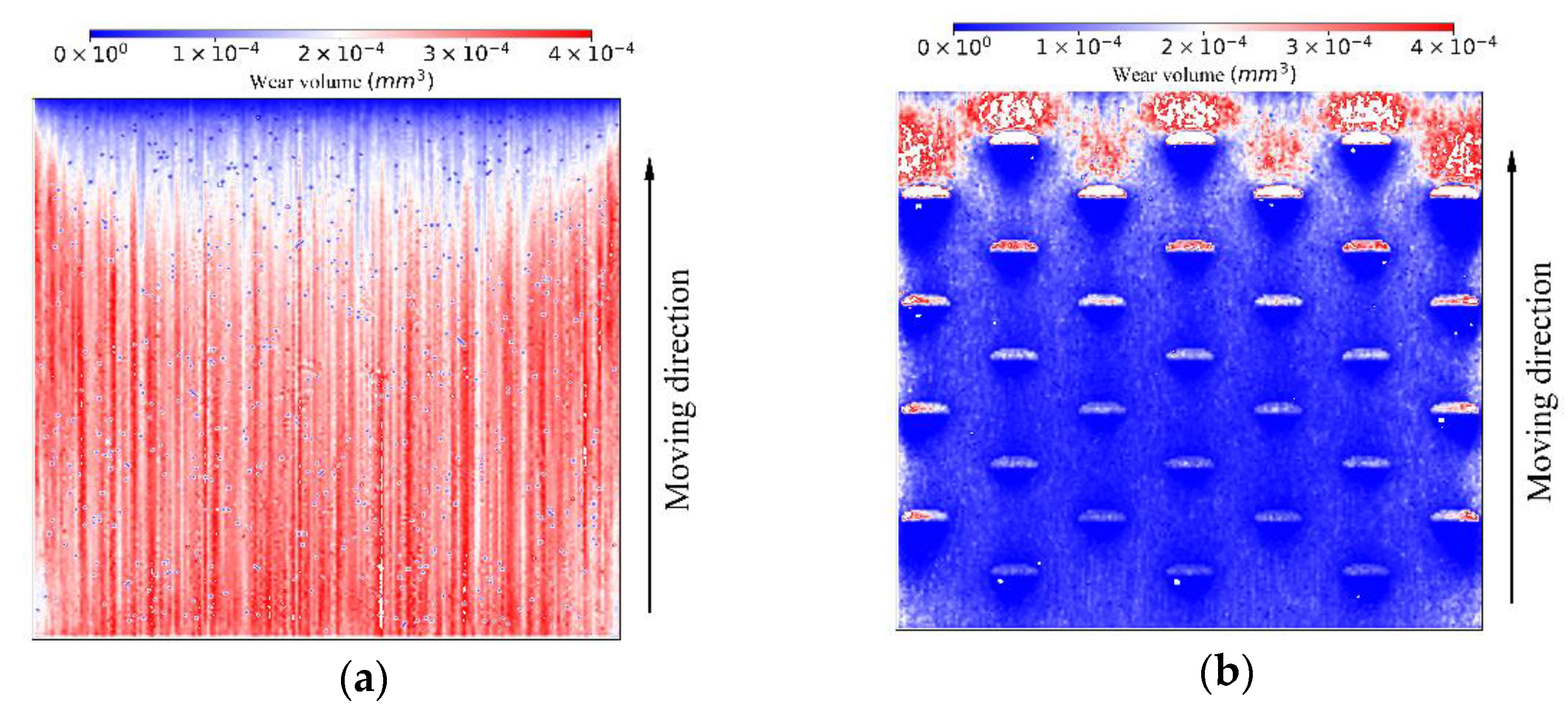
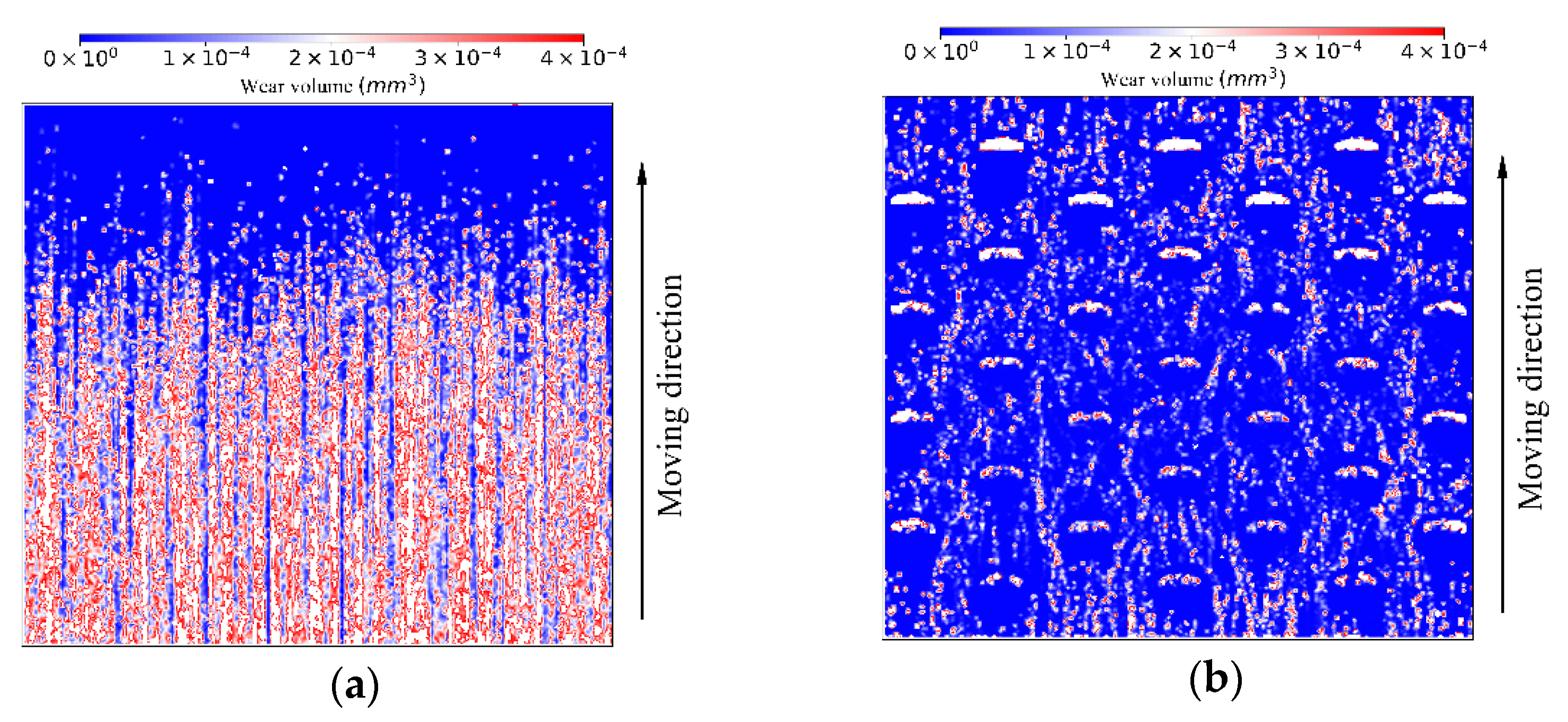
5.1.2. Bulk Flow and Sliding Wear Behavior

The bulk flow and sliding wear behavior, including the relative velocity of the particles and the relative wear rate, focus on the moving process of the samples. For comparison, the flat surface with the original particle bed (scaling factor is 1) was taken as a reference. It should be noted that Figure 13 and Figure 14 only present four scaling factors (1, 3, 5, and 7) to make the graphs more visible. As shown in Figure 13, the relative velocity, as indicated in Equation (10), increased rapidly for the first 700 mm and reached a relatively steady state until 1700 mm. For the relative wear rate (Equation (12)), as shown in Figure 14, a periodic fluctuation appeared from 100 mm to 1700 mm, and this phenomenon was magnified with the increase of the scaling factor. Combining both Figure 13 and Figure 14, the state of the simulations was considered to be stable in the range between 700 mm and 1700 mm.

Figure 15a indicates the average relative velocity of the particles. For the particle bed with a flat surface, the relative velocity was between 10% and 15% of the sample velocity with deviation of $\pm 1.5\%$, which means the particle size had a minor effect on bulk flow behavior. For the convex pattern surface, the relative velocity was higher than that of the flat surface, increasing from 30% to 45% from scaling factor 1 to 5 and decreasing to 40% from 5 to 8, and the standard deviation increased with the increase of the scaling factor from $\pm 0.4\%$ to $\pm 3.2\%$.

Figure 15b compares the relative wear rate between the convex pattern and flat surfaces. For the flat surface, the relative wear rate had a similar trend to the relative velocity and the standard deviation increased with the increase of the scaling factor. For the surface of the convex pattern, both the relative wear rate and standard deviation increased with an increasing scaling factor, and the deviation is lower than $\pm 5.5\%$ for all scaling factors.

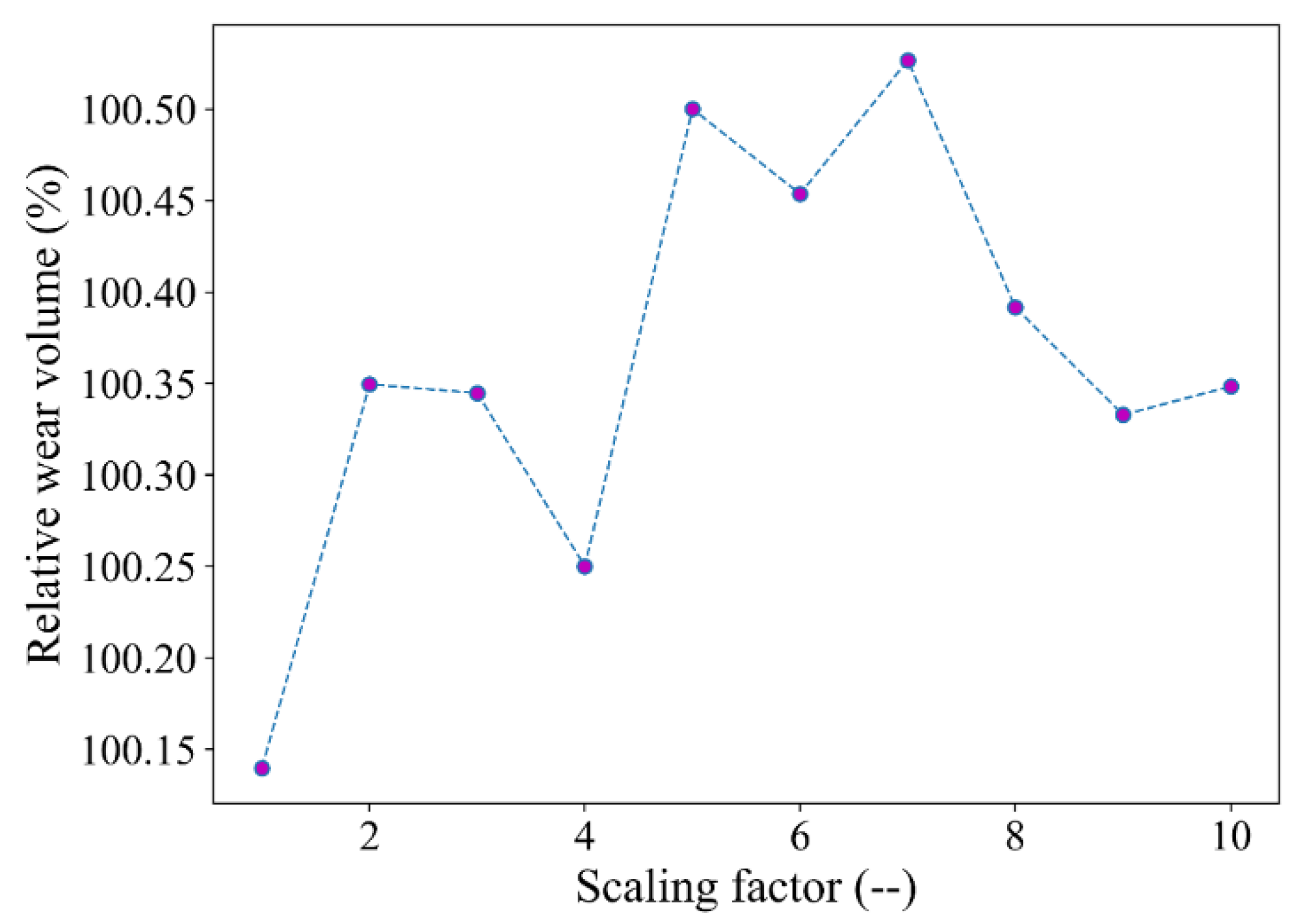
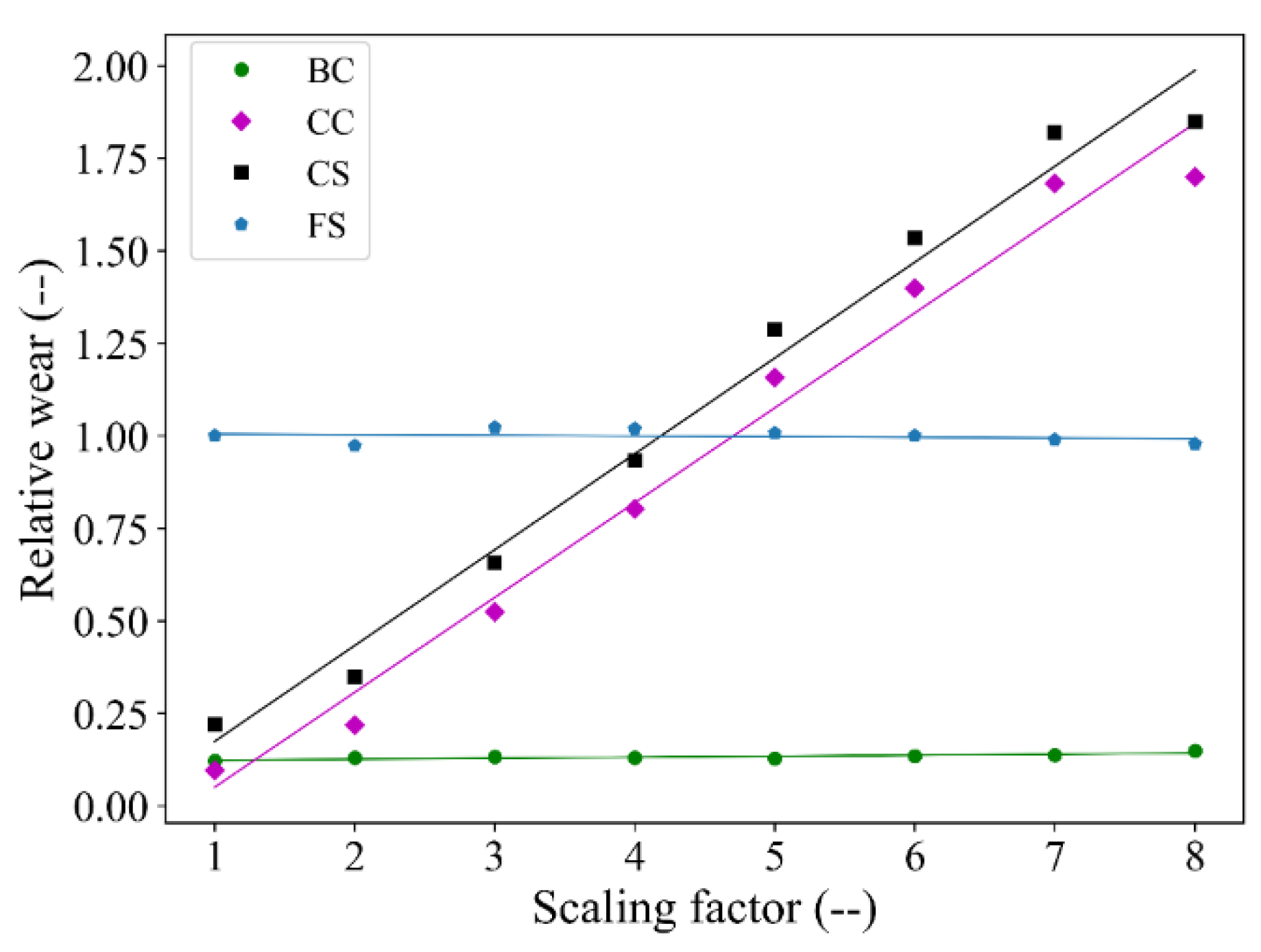
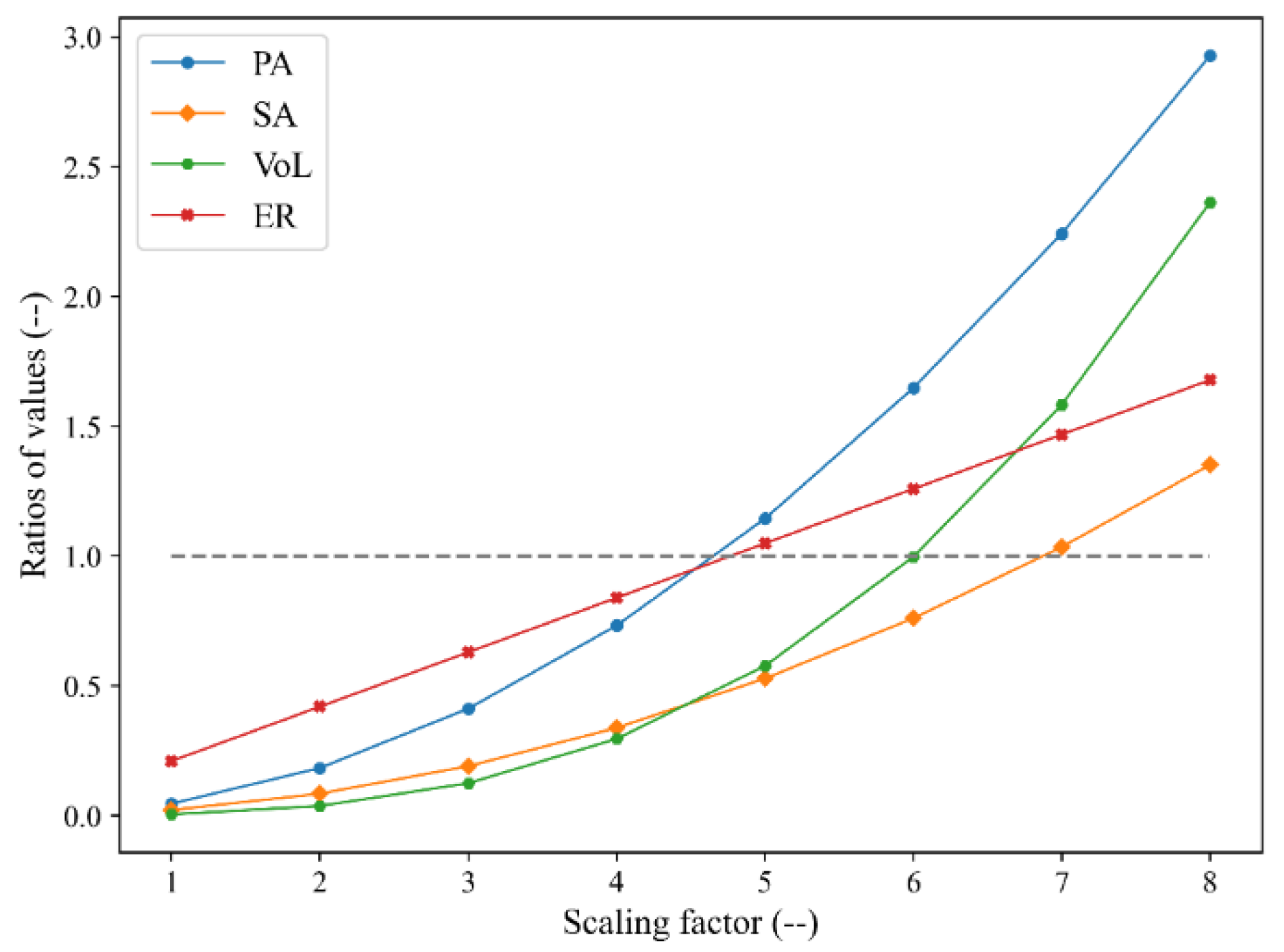
5.2. Sliding Wear Volume

The sliding wear volume is related to the wear volume of a flat surface caused by the original particles. Figure 16 shows the relative wear results, and the corresponding fitted models are listed in Equations (14)–(17). For the flat surface, the particle size had no influence on the sliding wear, as indicated by Equation (14). For the convex pattern surface, the total wear was linear to the particle size, as indicated by Equation (15). It can be seen that the relative wear of the convex pattern surface was lower than that of the flat surface when the scaling factor was lower than 4. This indicates that the convex pattern surface can both reduce and increase the sliding wear, and that the effect of the convex pattern surface was related to the particle size.

The convex pattern surface was separated into two parts, which are the base and the convex pattern. As shown in Figure 16, the base of the sample, as denoted by Equation (16), showed a similar trend to the flat surface and the wear was much lower than that of the flat surface, while the convex pattern, denoted by Equation (17), underwent the majority of the sliding wear and had a linear trend similar to that of the total wear of the convex pattern surface. This means that the base part was protected by transferring the sliding wear into the convex pattern.

$$y_{FS}=1.01-0.002x, R^2=0.96$$

(14)

$$y_{CS}=-0.08+0.26x, R^2=0.98$$

(15)

$$y_{BC}=0.12+0.003x, R^2=0.72$$

(16)

$$y_{CC}=-0.21+0.26x, R^2=0.98$$

(17)

Figure 17 compares the wear distributions between the flat and convex pattern surfaces for scaling factors 1 and 5. For a scaling factor of 1, as shown in Figure 17a, the wear distribution clearly shows that the scratches caused by the sliding of the particles were formed on the flat surface, especially in the back part of the sample. For the convex pattern surface, as shown in Figure 17b, the majority of wear was concentrated at the front part. Wear paths between two columns of the convex pattern from front to the back part of the sample can be visualized obviously, which indicates that the convex pattern can guide the particles to flow following specific paths and this guiding effect can lead to the rolling of particles to reduce the sliding wear. For detailed analysis of the wear distribution, please see the previous study [7].

For a scaling factor of 5, as shown in Figure 18a, the front part of the flat surface shows a larger area with less wear distributed compared to Figure 17a. For the convex pattern surface, the guiding effect of the convex pattern disappeared and the sliding wear was distributed on the whole sample. These phenomena are explained based on the particle velocity and angular velocity profiles in Section 5.3.

To study the relation between the particle size and the dimensions of the convex, four ratios, which are the projected area, surface area, volume, and equivalent radius, were investigated. For convex, the projected area was the area of a convex projected vertically. The equivalent radius was obtained when taking the convex as a half-sphere. It should be noted that these parameters of particles are based on the values of $R_{50}$ (particle radius corresponding to 50% of cumulative mass). The four ratios are shown in Equations (18)–(21):

$${\alpha }_{ER}=R_p/\sqrt[3]{abh/2}$$

(18)

$${\alpha }_{PA}=R_p^2/\left(ab\right)$$

(19)

$${\alpha }_{SA}=6R_p^2/\left(ab+ah+bh\right)$$

(20)

$${\alpha }_v=2R_p^3/\left(abh\right)$$

(21)

where $R_p$, $a$, $b$, and $h$ are the radius of particle, major radius, minor radius, and height of the convex pattern, respectively. ${\alpha }_{ER}$,${\alpha }_{PA}$,${\alpha }_{SA}$, and ${\alpha }_v$ are the ratios of the equivalent radius, projected area, surface area, and volume of particle to that of the convex pattern, respectively.

Figure 19 shows that a scaling factor of 4 is a critical value, where the wear results for the flat and convex pattern surfaces are comparable. It can be seen that ${\alpha }_{SA}$ and ${\alpha }_v$ have no direct relationship with the sliding wear. ${\alpha }_{ER}$ and ${\alpha }_{PA}$ present an obvious relationship with the wear result, which shows that the convex pattern surface can reduce the sliding wear when the ratios are less than 1 and increase the sliding wear when they are higher than 1. Taking the linear relationship between the relative wear and the scaling factor shown in Figure 16 into account, it can be seen that the ${\alpha }_{ER}$ determines the effect of the surface of the convex pattern on the reduction of sliding wear. When ${\alpha }_{ER}$ is lower than 1, the convex pattern promotes the rolling effect on particles. When ${\alpha }_{ER}$ is higher than 1, the particles travel over the convex pattern, which becomes the resistance of the movement of particles.

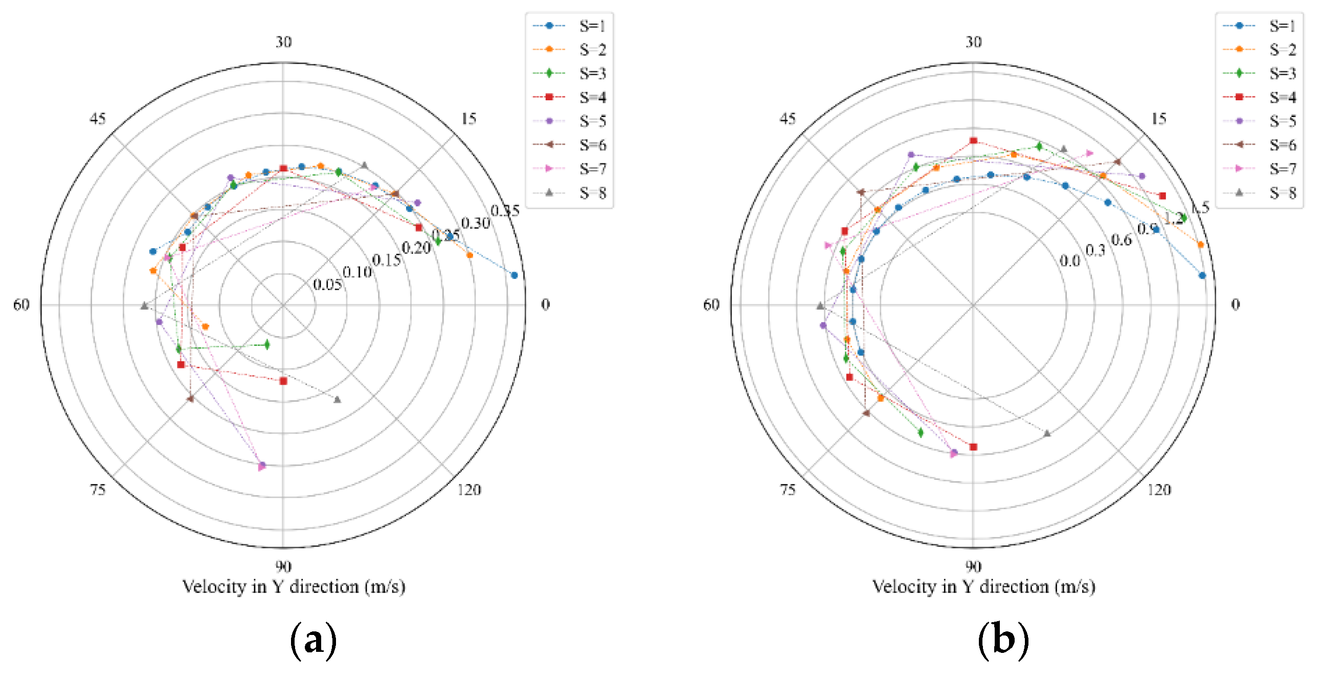
5.3. Bulk Flow Behavior

The bulk flow behavior, including the velocity and angular velocity of the particles, is used to indicate the guiding and rolling effect of the convex pattern. It should be noted that the bulk flow behavior only focuses on the particles in the moving bins, as shown in Figure 10.

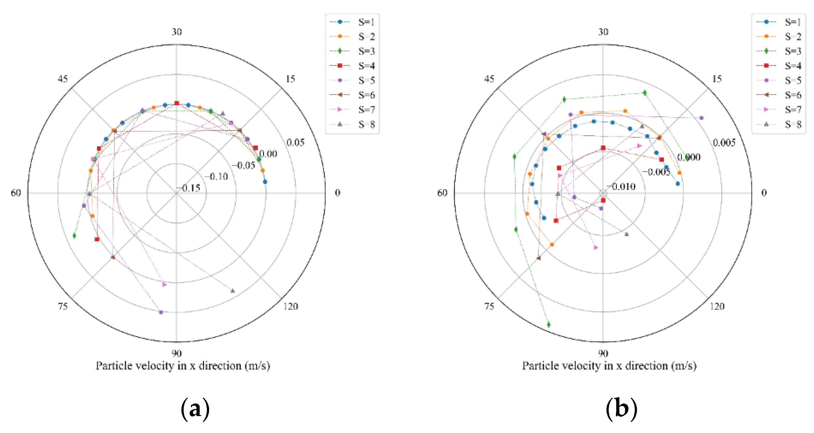
5.3.1. Velocity Behavior

The velocity profile is displayed by spider charts, where the values outside the charts and in the radius direction are the particle bed height and velocity or angular velocity of particles. As the particle size varies, the layer depth, as shown in Table 2, differs for different scaling factors.

The particle velocity in the y-direction shows the tendency of particles to move with the sample. For a flat surface, as shown in Figure 20a, the particle velocity for all scaling factors is less than $0.35 \mathrm{m}/\mathrm{s}$ and much lower than the sample velocity $2 \mathrm{m}/\mathrm{s}$. This means that the particle size has a minor influence on the particle velocity in the y-direction. Moreover, the particle velocity decreases with the increase in the height of the particle bed as the influence of the sample weakens.

For the convex pattern surface, as shown in Figure 20a, it shows that the velocity in the bottom bin is higher than $0.9 \mathrm{m}/\mathrm{s}$ for all scaling factors, which is much higher than that of the flat surface. This indicates that the particles at the bottom of the particle bed have a tendency to move with the sample to reduce the sliding distance. This tendency is more obvious for low scaling factors because smaller particles are easier to be guided by the convex pattern. In addition, the effect drops abruptly with the increase in particle bed height.

The velocity of the particles in the Z direction indicates the tendency of the particles to move across layers. For the flat surface, as shown in Figure 21a, the velocity of the particles was much lower than that of the surface of the convex pattern, as shown in Figure 21b, which means that the flat surface had a weaker influence on the movement of particles across bins. For the convex pattern surface, Figure 21b shows that the particle velocity increased to a maximum value from the bottom layer and decreased to the top layer for all scaling factors. The velocity at the bottom layer increased with the increase of the scaling factor, which indicates that the larger particles could travel over the convex pattern, while the smaller particles moved around the convex pattern. This means that the guiding and rolling effect decreased with an increasing particle size and this phenomenon can explain the wear distribution, as shown in Figure 17 and Figure 18.

The particle velocity in the X direction showed a tendency of the particles to move sideways. For both the flat and convex pattern surfaces, as shown in Figure 22, the particles had no obvious tendency to move sideways for all scaling factors. For each scaling factor, the particles had comparable velocity at all layers, so the effect of the samples on the movement of particles in the X direction can be ignored.

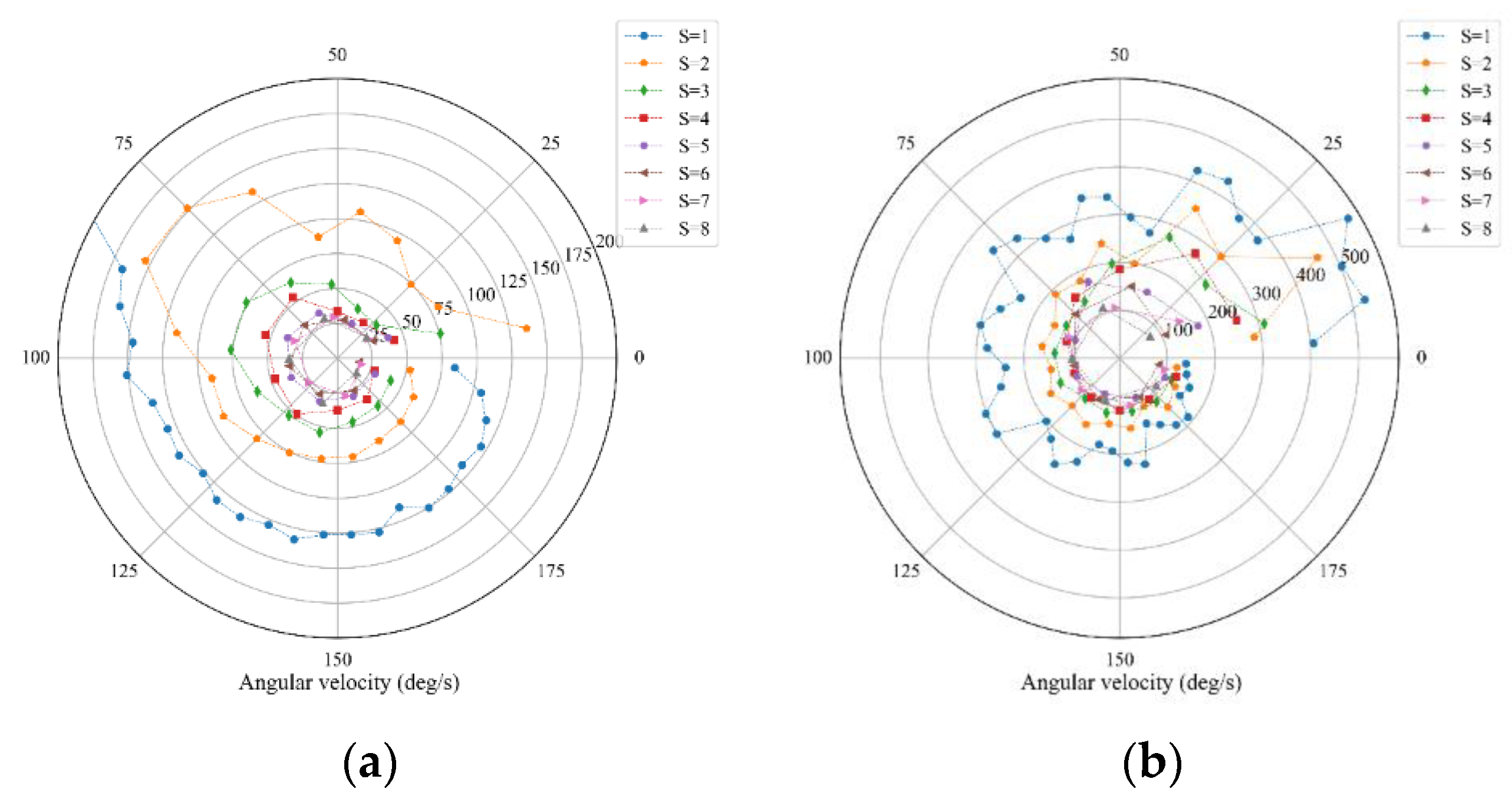
5.3.2. Angular Velocity Behavior

The angular velocity was analyzed with a different bin group, as shown in Figure 23. The angular velocity focuses on the bottom layer of particles, as the bottom layer reflects the rolling and guiding effect of the convex pattern. The depth and width of each bin are related to the scaling factor and equal to the depth of the bin, as shown in Figure 10.

For the flat surface, the angular velocity of the particles decreased dramatically with an increasing scaling factor, as shown in Figure 24a. For each scaling factor, the angular velocity experienced two increase-drop periods. First, the angular velocity showed a high value at the first bin and dropped to a low value at the second bin. Second, the angular velocity increased again from the second bin to the maximum value and gradually dropped to the lowest value until the last bin. This is because the initial contact between the particles and the sample induced rotation of the particles, after which this effect was quickly weakened. As high angular velocity tended to generate less sliding wear, this phenomenon can explain the lower wear distribution in the front part of the flat surface sample.

For the surface of the convex pattern, as shown in Figure 24b, the angular velocity was much higher than that of the corresponding flat surface, decreasing with an increasing scaling factor. This indicates that the rolling effect of the convex pattern decreased with the increase of particle size. The particles at the front part of the sample have a higher angular velocity compared with those at the back part for all scaling factors, and this means that the rolling effect weakens from the front to the back of the sample.

6. Conclusions

This paper investigated the influence of the particle size on the sliding wear of a convex pattern surface for the interaction between bulk material and bulk handling equipment. On the basis of the coarse graining technique, the relationship between the dimensions of the convex pattern and the particle size is clarified and the effect of the convex pattern on the flow behavior of particles is elaborated.

The simulation system reaches a steady state from 700 mm to 1700 mm. For a flat surface, the particle relative velocity and relative wear rate of the sample are comparable and the corresponding deviations are less than $\pm 0.65\%$ and $\pm 3.3\%$, respectively. For the convex pattern surface, the particle size obviously influences the bulk flow behavior and relative wear, while the corresponding deviations are less than $\pm 1.2\%$ and $\pm 5.5\%$, respectively, for all scaling factors.

The particle size has no effect on the sliding wear of the flat surface, while it has a linear relationship with the sliding wear for the convex pattern surface. Most of the sliding wear of the convex pattern surface occurs on the convex part, and the base of the sample is protected by transferring the sliding wear to the convex.

The convex pattern surface enables to reduce the sliding wear compared with the flat surface when the scaling factor is lower than 4. The ratio (${\alpha }_{ER}$) of the equivalent radius of the convex to the particle radius determines the effect of the convex pattern surface. When ${\alpha }_{ER}$ is lower than 1, the convex pattern can reduce the sliding wear through the guiding and rolling effect. When ${\alpha }_{ER}$ is higher than 1, particles can travel across the convex pattern, which becomes the resistance of the particles.

The investigated convex pattern surfaces can, in some cases, significantly accelerate the flowing and rolling of particles compared with the flat surface. It should be noted that only the flow behavior cannot fully reflect the effect of the convex pattern on the sliding wear.

In conclusion, when the relationship between particle size and the dimensions of the convex pattern is carefully considered, the convex pattern surface can reduce the sliding wear dramatically. Future research including sliding wear experiments on a circular wear tester to verify the simulation results will be conducted.

References

1. Schulze, D. Powders and Bulk Solids: Behavior, Characterization, Storage and Flow; Springer: Berlin/Heidelberg, Germany, 2008; pp. 198–230. [Google Scholar]
2. Svanberg, A.; Larsson, S.; Mäki, R.; Jonsén, P. Full-scale simulation and validation of wear for a mining rope shovel bucket. Minerals 2021, 11, 623. [Google Scholar] [CrossRef]
3. Esteves, P.M.; Mazzinghy, D.B.; Galéry, R.; Machado, L.C.R. Industrial vertical stirred mills screw liner wear profile compared to discrete element method simulations. Minerals 2021, 11, 397. [Google Scholar] [CrossRef]
4. Andrejiova, M.; Grincova, A.; Marasova, D. Measurement and simulation of impact wear damage to industrial conveyor belts. Wear 2016, 368–369, 400–407. [Google Scholar] [CrossRef]
5. Roberts, A.W. Chute performance and design for rapid flow conditions. Chem. Eng. Technol. 2003, 26, 163–170. [Google Scholar] [CrossRef]
6. Chen, G. Surface Wear Reduction of Bulk Solids Handling Equipment Using Bionic Design. Ph.D. Thesis, Delft University of Technology, Delt, The Netherlands, 2017. [Google Scholar]
7. Yan, Y.; Helmons, R.; Wheeler, C.; Schott, D. Optimization of a convex pattern surface for sliding wear reduction based on a definitive screening design and discrete element method. Powder Technol. 2021, 394, 1094–1110. [Google Scholar] [CrossRef]
8. Schramm, F.; Kalácska, Á.; Pfeiffer, V.; Sukumaran, J.; De Baets, P.; Frerichs, L. Modelling of abrasive material loss at soil tillage via scratch test with the discrete element method. J. Terramechanics 2020, 91, 275–283. [Google Scholar] [CrossRef]
9. Kalácska, Á.; De Baets, P.; Fauconnier, D.; Schramm, F.; Frerichs, L.; Sukumaran, J. Abrasive wear behaviour of 27MnB5 steel used in agricultural tines. Wear 2020, 442–443, 203107. [Google Scholar] [CrossRef]
10. Phan, T.H.; Tieu, A.K.; Zhu, H.T.; Kosasih, B.Y.; Wu, Q.; Fan, Q.; Sun, D.L. A Study of Abrasive Wear on High Speed Steel Surface in Hot Rolling. Appl. Mech. Mater. 2016, 846, 589–594. [Google Scholar] [CrossRef]
11. Franke, J.; Cleary, P.W.; Sinnott, M.D. How to account for operating condition variability when predicting liner operating life with DEM—A case study. Miner. Eng. 2015, 73, 53–68. [Google Scholar] [CrossRef]
12. Perazzo, F.; Löhner, R.; Labbe, F.; Knop, F.; Mascaró, P. Numerical modeling of the pattern and wear rate on a structural steel plate using DEM. Miner. Eng. 2019, 137, 290–302. [Google Scholar] [CrossRef]
13. Powell, M.S.; Weerasekara, N.S.; Cole, S.; Laroche, R.D.; Favier, J. DEM modelling of liner evolution and its influence on grinding rate in ball mills. Miner. Eng. 2011, 24, 341–351. [Google Scholar] [CrossRef]
14. Ma, S.; Niu, C.; Yan, C.; Tan, H.; Xu, L. Discrete element method optimisation of a scraper to remove soil from ridges formed to cold-proof grapevines. Biosyst. Eng. 2021, 210, 156–170. [Google Scholar] [CrossRef]
15. Katinas, E.; Chotěborský, R.; Linda, M.; Jankauskas, V. Wear modelling of soil ripper tine in sand and sandy clay by discrete element method. Biosyst. Eng. 2019, 188, 305–319. [Google Scholar] [CrossRef]
16. Phan, H.T.; Tieu, A.K.; Zhu, H.; Kosasih, B.; Zhu, Q.; Grima, A.; Ta, T.D. A study of abrasive wear on high speed steel surface in hot rolling by Discrete Element Method. Tribol. Int. 2017, 110, 66–76. [Google Scholar] [CrossRef]
17. Feng, Y.T.; Owen, D.R.J. Discrete element modelling of large scale particle systems—I: Exact scaling laws. Comput. Part. Mech. 2014, 1, 159–168. [Google Scholar] [CrossRef] [Green Version]
18. Feng, Y.T.; Han, K.; Owen, D.R.J.; Loughran, J. On upscaling of discrete element models: Similarity principles. Eng. Comput. 2009, 26, 599–609. [Google Scholar] [CrossRef]
19. Grima, A.P.; Wypych, P.W. Development and validation of calibration methods for discrete element modelling. Granul. Matter 2011, 13, 127–132. [Google Scholar] [CrossRef] [Green Version]
20. Nasato, D.S.; Goniva, C.; Pirker, S.; Kloss, C. Coarse graining for large-scale DEM simulations of particle flow—An investigation on contact and cohesion models. Procedia Eng. 2015, 102, 1484–1490. [Google Scholar] [CrossRef] [Green Version]
21. Mohajeri, M.J.; Helmons, R.L.J.; van Rhee, C.; Schott, D.L. A hybrid particle-geometric scaling approach for elasto-plastic adhesive DEM contact models. Powder Technol. 2020, 369, 72–87. [Google Scholar] [CrossRef]
22. Queteschiner, D.; Lichtenegger, T.; Pirker, S.; Schneiderbauer, S. Multi-level coarse-grain model of the DEM. Powder Technol. 2018, 338, 614–624. [Google Scholar] [CrossRef]
23. Schott, D.L.; Lommen, S.W.; van Gils, R.; de Lange, J.; Kerklaan, M.M.; Dessing, O.M.; Vreugdenhil, W.; Lodewijks, G. Scaling of particles and equipment by experiments of an excavation motion. Powder Technol. 2015, 278, 26–34. [Google Scholar] [CrossRef]
24. Roessler, T.; Katterfeld, A. Scaling of the angle of repose test and its influence on the calibration of DEM parameters using upscaled particles. Powder Technol. 2018, 330, 58–66. [Google Scholar] [CrossRef]
25. Robinson, M.; Ramaioli, M.; Luding, S. Fluid-particle flow simulations using two-way-coupled mesoscale SPH-DEM and validation. Int. J. Multiph. Flow 2014, 59, 121–134. [Google Scholar] [CrossRef] [Green Version]
26. Lommen, S.; Mohajeri, M.; Lodewijks, G.; Schott, D. DEM particle upscaling for large-scale bulk handling equipment and material interaction. Powder Technol. 2019, 352, 273–282. [Google Scholar] [CrossRef]
27. Thakur, S.C.; Ooi, J.Y.; Ahmadian, H. Scaling of discrete element model parameters for cohesionless and cohesive solid. Powder Technol. 2016, 293, 130–137. [Google Scholar] [CrossRef] [Green Version]
28. Weinhart, T.; Labra, C.; Luding, S.; Ooi, J.Y. Influence of coarse-graining parameters on the analysis of DEM simulations of silo flow. Powder Technol. 2016, 293, 138–148. [Google Scholar] [CrossRef]
29. Cai, R.; Zhao, Y. An experimentally validated coarse-grain DEM study of monodisperse granular mixing. Powder Technol. 2020, 361, 99–111. [Google Scholar] [CrossRef]
30. Widartiningsih, P.M.; Mori, Y.; Takabatake, K.; Wu, C.Y.; Yokoi, K.; Yamaguchi, A.; Sakai, M. Coarse graining DEM simulations of a powder die-filling system. Powder Technol. 2020, 371, 83–95. [Google Scholar] [CrossRef]
31. Solutions, D.E.M. EDEM 2.3 User Guide; DEM Solutions Ltd.: Edinburgh, Scotland, UK, 2010. [Google Scholar]
32. Antypov, D.; Elliott, J.A. On an analytical solution for the damped Hertzian spring. EPL 2011, 94, 5004. [Google Scholar] [CrossRef] [Green Version]
33. Ai, J.; Chen, J.F.; Rotter, J.M.; Ooi, J.Y. Assessment of rolling resistance models in discrete element simulations. Powder Technol. 2011, 206, 269–282. [Google Scholar] [CrossRef]
34. Archard, J.F. Contact and rubbing of flat surfaces. J. Appl. Phys. 1953, 24, 981–988. [Google Scholar] [CrossRef]
35. Ramalho, A.; Miranda, J.C. The relationship between wear and dissipated energy in sliding systems. Wear 2006, 260, 361–367. [Google Scholar] [CrossRef] [Green Version]
36. Forsström, D.; Jonsén, P. Calibration and validation of a large scale abrasive wear model by coupling DEM-FEM: Local failure prediction from abrasive wear of tipper bodies during unloading of granular material. Eng. Fail. Anal. 2016, 66, 274–283. [Google Scholar] [CrossRef]
37. Yu, A.B.; An, X.Z.; Zou, R.P.; Yang, R.Y.; Kendall, K. Self-assembly of particles for densest packing by mechanical vibration. Phys. Rev. Lett. 2006, 97, 95–98. [Google Scholar] [CrossRef]
38. An, X.Z.; Yang, R.Y.; Zou, R.P.; Yu, A.B. Effect of vibration condition and inter-particle frictions on the packing of uniform spheres. Powder Technol. 2008, 188, 102–109. [Google Scholar] [CrossRef]
39. Chen, X.; Liu, Y. Finite Element Modeling and Simulation with ANSYS Workbench; CRC Press: Boca Raton, FL, USA, 2014. [Google Scholar]
40. Chen, G.; Schott, D.L.; Lodewijks, G. Sensitivity analysis of DEM prediction for sliding wear by single iron ore particle. Eng. Comput. 2017, 34, 2031–2053. [Google Scholar] [CrossRef] [Green Version]
Figure 1. Sample of river gravel.
Minerals 12 00139 g001
Figure 2. Particle size distribution.
Minerals 12 00139 g002
Figure 3. Packing container.
Minerals 12 00139 g003
Figure 4. Coordination number distribution. (a) Before vibration; (b) After vibration; (c) Difference of coordination number after and before vibration.
Minerals 12 00139 g004
Figure 5. Porosity distribution. (a) Before vibration; (b) After vibration; (c) Difference of porosity after and before vibration.
Minerals 12 00139 g005
Figure 6. Pin-on-disc test setup. (a) Top view; (b) Side view.
Minerals 12 00139 g006
Figure 7. Comparison between the simulation results and Archard wear model.
Minerals 12 00139 g007
Figure 8. Meshed convex pattern sample (a: major radius; b: minor radius; c: vertical distance; d: horizontal distance; h: height of convex) [7].
Minerals 12 00139 g008
Figure 9. Original particle bed.
Minerals 12 00139 g009
Figure 10. Moving bins.
Minerals 12 00139 g010
Figure 11. Coordination number distribution.
Minerals 12 00139 g011
Figure 12. Porosity distribution.
Minerals 12 00139 g012
Figure 13. Relative velocity of the particles for the convex pattern surface.
Minerals 12 00139 g013
Figure 14. Relative wear rate of the convex pattern surface.
Minerals 12 00139 g014
Figure 15. Comparison of the relative velocity and wear rate. (a) Relative velocity; (b) Relative wear rate.
Minerals 12 00139 g015
Figure 16. Relative wear vs. scaling factor (CS: convex pattern surface, FS: flat surface, BC: base of CS, CC: convex part of CS).
Minerals 12 00139 g016
Figure 17. Wear distribution of samples for a scaling factor of 1. (a) Flat surface; (b) Convex pattern surface.
Minerals 12 00139 g017
Figure 18. Wear distribution of samples for a scaling factor of 5. (a) Flat surface; (b) Convex pattern surface.
Minerals 12 00139 g018
Figure 19. Ratios of values between d 50 related to convex pattern related (PA: projected area, SA: surface area, Vol: volume, ER: equivalent radius).
Minerals 12 00139 g019
Figure 20. Particle velocity in the y-direction. (a) Flat surface; (b) Convex pattern surface.
Minerals 12 00139 g020
Figure 21. Particle velocity in Z direction. (a) Flat surface; (b) Convex pattern surface.
Minerals 12 00139 g021
Figure 22. Particle velocity in the X direction. (a) Flat surface; (b) Convex pattern surface.
Minerals 12 00139 g022
Figure 23. Bin groups for the angular velocity.
Minerals 12 00139 g023
Figure 24. Angular velocity. (a) Flat surface; (b) Convex pattern surface.
Minerals 12 00139 g024