Article

Automated Hyperparameter Optimization of Gradient Boosting Decision Tree Approach for Gold Mineral Prospectivity Mapping in the Xiong’ershan Area

1
MNR Key Laboratory of Metallogeny and Mineral Resource Assessment, Institute of Mineral Resources, Chinese Academy of Geological Sciences, Beijing 100037, China
2
Institute of Geological Survey, China University of Geosciences, Wuhan 430074, China
3
China Aero Geophysical Survey and Remote Sensing Center for Natural Resources, Beijing 100083, China
4
Institute of Earth Science, China University of Geosciences, Beijing 100083, China
*
Authors to whom correspondence should be addressed.
Minerals 2022, 12(12), 1621; https://doi.org/10.3390/min12121621
Submission received: 1 November 2022 / Revised: 13 December 2022 / Accepted: 14 December 2022 / Published: 16 December 2022
(This article belongs to the Special Issue Genesis and Metallogeny of Non-ferrous and Precious Metal Deposits)

Abstract

:
The weak classifier ensemble algorithms based on the decision tree model, mainly include bagging (e.g., fandom forest-RF) and boosting (e.g., gradient boosting decision tree, eXtreme gradient boosting), the former reduces the variance for the overall generalization error reduction while the latter focuses on reducing the overall bias to that end. Because of its straightforward idea, it is prevalent in MPM (mineral prospectivity mapping). However, an inevitable problem in the application of such methods is the hyperparameters tuning which is a laborious and time-consuming task. The selection of hyperparameters suitable for a specific task is worth investigating. In this paper, a tree Parzen estimator-based GBDT (gradient boosting decision tree) model (TPE-GBDT) was introduced for hyperparameters tuning (e.g., loss criterion, n_estimators, learning_rate, max_features, subsample, max_depth, min_impurity_decrease). Then, the geological data of the gold deposit in the Xiong ‘ershan area was used to create training data for MPM and to compare the TPE-GBDT and random search-GBDT training results. Results showed that the TPE-GBDT model can obtain higher accuracy than random search-GBDT in a shorter time for the same parameter space, which proves that this algorithm is superior to random search in principle and more suitable for complex hyperparametric tuning. Subsequently, the validation measures, five-fold cross-validation, confusion matrix and success rate curves were employed to evaluate the overall performance of the hyperparameter optimization models. The results showed good scores for the predictive models. Finally, according to the maximum Youden index as the threshold to divide metallogenic potential areas and non-prospective areas, the high metallogenic prospect area (accounts for 10.22% of the total study area) derived by the TPE-GBDT model contained > 90% of the known deposits and provided a preferred range for future exploration work.

1. Introduction

Mineral prospectivity mapping (MPM) can guide us to conduct deep and peripheral ore prospecting in chosen study area. From the spatial dimension, it can be divided into two-dimensional MPM and three-dimensional MPM [1,2]. Two-dimensional MPM can facilitate the regional-scale prospecting and delineation of the prospective area [3,4,5,6,7,8], while three-dimensional MPM can be used to guide the delineation of the deep metallogenic target area at the deposit scale [9,10,11,12,13,14,15,16]. In terms of methods, MPM can be divided into knowledge-driven MPM and data-driven MPM. Knowledge-driven MPM is mainly based on geological expert experience for statistical analysis methods [17,18,19,20,21,22,23,24], and data-driven MPM is mainly based on big data methods (i.e., machine learning or deep learning algorithms) [25,26,27,28,29,30,31,32,33,34,35].
No matter which MPM is performed, at either the regional scale or at the deposit scale, MPM is carried out by way of data-driven or knowledge-driven approaches, geological exploration data are essential. The quality of exploration data collected matters a great deal for the accuracy of MPM. However, the geoscientific data available are generally limited, and there are a few target/positive samples (ore spots) in the real world. Moreover, machine learning and deep learning algorithms are data-hungry [36,37,38,39,40,41]. Therefore, there are some inevitable problems for the application of big data algorithms based on geological data (such as with the data structure, extreme imbalance of positive (prospect) and negative samples (non-prospect) etc.) [42].
In resolving these problems, the current research mainly focused on data augmentation and algorithm optimization, among which the data augmentation mainly included: multi-sample data augmentation (e.g., under-sampling, over-sampling, synthetic sampling) [43,44,45,46,47,48,49,50,51], single-sample data augmentation (e.g., image up-and-down, left-right inversion and center inversion, etc.) [52,53,54,55,56,57], and unsupervised data enhancement (e.g., GAN, AutoML) [58,59,60,61]. The improved algorithms mainly included design cost sensitive functions and used ensemble learning, such as cost-sensitive neural networks [62,63], balanced fuzzy support vector machine algorithms [64,65,66,67,68], a CBP-SVM algorithm based on a hybrid model [69], the RSBoost algorithm [70,71,72], anomaly detection algorithms (e.g., isolation forest) [73,74,75,76], differential Siamese convolutional neural network [77,78,79,80,81], and the MLA (machine learning algorithms) based on the decision tree model (e.g., GBDT, weighted random forest) [82,83,84]. Among them, the tree model was suitable for few-shot data training [85,86,87].
The MLA based on the tree model has high computational efficiency and strong model discrimination ability with a simple principle. It is one of the few “white box models” in MLA [88,89,90,91]. Moreover, in terms of the function of the tree model itself, the decision tree can be used for classification and regression, which also produce additional criteria such as importance of features and continuous variable box indexes. In ensemble learning, the tree model is the most commonly used primary classifier [92]. These advantages make the tree model one of the most important in MLA. The GBDT model is an essential boosting algorithm, based on a decision tree, that utilizes the strategy of multi-model integration to fit the residuals for reducing the deviation and variance of the model [93,94]. Nevertheless, it is also faced with an important problem: hyperparametric optimization (HPO). However, there are few studies on HPO with GBDT. Many researchers tend to set default parameters values for the model, leading to weak end results [95,96]. The optimization of hyperparameters, for certain case studies, has a great impact on the effectiveness of the algorithm, and it plays a crucial role in the accuracy and generalization ability of the final generated model. There are a large number of hyperparameters (e.g., n_estimation, learning_rate, max_features, subsample, etc.) in the GBDT, with different parameters having different effects on the GBDT model. Therefore, the selection of the hyperparameter combination is important to achieve the optimal model.
With regard to its algorithms, we aspire to eventually realize the perfect automation of all processes. The discipline specializing in automation machine learning is called AutoML, and hyperparameter automatic optimization is the most mature, in-depth, and well-known direction [97,98,99]. Theoretically, when the computational power and data are sufficient, the performance of HPO should exceed that of human beings. HPO can reduce human workload, and the results obtained by HPO are more likely to be reproduced than searched, so HPO can greatly improve the reproducibility and fairness of scientific research [100,101,102,103]. Contemporary HPO algorithms can be mainly divided into grid-based search (grid), Bayesian optimization (Bayesian), gradient-based optimization (gradient-based), and population-based optimization (evolutionary algorithm, genetic algorithm, etc.), among which the grid search and Bayes-based optimization are the most popular [104,105,106,107,108,109,110]. These HPO methods have great effect and significance on optimizing complex ensemble algorithms.
In this paper, a knowledge-driven synthetic sampling method was proposed for dealing with imbalanced data, which made the data form more suitable for MLA. The GBDT algorithm based on the decision tree model for few-shot geological data was selected. The random grid search and the Bayesian optimization based on the TPE algorithm were used to study the hyperparametric of the GBDT model, taking the gold deposit in Xiong ‘ershan area as an example, in order to verify the difference of MPM based on two algorithms for HPO with few shot geological data. The study can be used as a reference for the research of MLA based on HPO in the MPM.

2. Methodology

2.1. GBDT Algorithm

The gradient boosting decision tree (GBDT) is a representative boosting algorithm, which is the cornerstone of XGBoost, LightGBM and other tree model algorithms. It is also one of the most widely used MLAs in the industry and the most stable one in practice. When it was first proposed, GBDT was written as gradient boosting machine (GBM), which integrated bagging and boosting ideas and can accept all types of weak estimators as input. After the weak estimator was defined as a decision tree, it was slowly renamed the gradient boosting tree.
Inspired by the boosting algorithm, GBDT naturally contains three boosting elements: loss function L   ( x , y ) , weak estimators   f   ( x )   and comprehensive integration results   H   ( x ) [111]. Yet, some improvements have since been made: (1) The weak estimator output type of GBDT is no longer consistent with the ensemble algorithm. For AdaBoost or random forest (RF) algorithms, weak estimators are regressions when ensemble algorithms perform regression tasks. When ensemble algorithms perform classification tasks, weak estimators are classifiers; no matter whether the GBDT is performing regression or classification tasks as a whole, the weak estimator must be a regression. It outputs specific classification results by sigmoid or softmax functions, but the actual weak estimator must be a regression; (2) The loss function has been extended to any differentiable function in the mathematical principle, and is no longer limited to a fixed or single loss function; (3) Before each weak estimator is established, the sample weight is not modified, but the residual error is fitted to affect the structure of the subsequent weak estimator; (4) It joins the idea of random sampling from RF, allowing samples and features to be sampled before each tree is built to increase the independence between weak estimators (thus allowing for out-of-bag datasets to be used to verify the establishment results of each weak evaluator). It can further increase the stability of boosting algorithm.
As is well known, MPM is considered a classification problem in the MLA, and is categorized as either a prospect or non-prospect in the study region. So, we should know the GBDT binary classification algorithm flow [112]:
First, initialize weak classifier as:
H 0 = log P ( Y = 1 | x )   1 P ( Y = 1 | x )  
where the P   ( Y = 1 | x ) is the proportion of positive (as y = 1) in train datasets, using prior information to initialize the learner.
Second, the loss function is defined, and the GBDT binary classification algorithm uses a logarithmic loss function:
L ( θ ) = y i log y i ^ ( 1 y i ) log ( 1 y i ^ )
where the y i ^ is the result of logistic regression prediction   H   ( x ) .
H ( x ) = 1 1 + e f ( x )  
where the   f   ( x )   are the weak estimators. Flowing Formula (3) into Formula (2) as:
L ( y i ,   f ( x i ) ) = y i log ( 1 + e f ( x i )   ) + ( 1 y i ) [ f ( x i ) + log ( 1 + e f   ( x i )   )   ]
Then, calculation of negative gradient of loss function (pseudo residual):
r m , i = | L ( y i , f ( x i ) )   f ( x i )   | f ( x ) =   f m 1 ( x )   = y i 1 1 + e f ( x )   = y i y i ^
Subsequently, calculate the best residual fitting value of each leaf node as:
C m , j = argmin x i R m , j L ( y i , f m 1 ( x i ) + C )  
where the m is the mth trees. In order to solve the C m , j value, we introduce the second-order Taylor expansion as:
C m , j = x i R m , j r m , i x i R m , j ( y i r m , i ) ( 1 y i + r m , i )  
Meanwhile, update strong learners as:
H m = H m 1 ( x ) + j = 1 J m C m , j I ( x R m , j )  
Finally, the H M   ( x )   as:
  H M   ( x ) = H m + m = 1 M j = 1 J m C m , j I ( x R m , j )  
In summary, the GBDT binary classification algorithm uses multiple CART regression trees to fit the log probability with the positive label (as y = 1), and the loss function uses the logarithmic loss, but it is necessary to replace the predicted value y i ^ (the probability predicted as y = 1) with the logarithmic probability   H   ( x )   predicted by the regression tree, and then fit the residuals each round. After the final classifier output is obtained, the probability that the prediction label is positive (as y = 1) can be obtained by the sigmoid function.

2.2. Hyperparameter Optimization Method

Model optimization is one of the most difficult challenges in MLA implementation. Parameter adjustment is the core of model optimization, but the process is complex and cumbersome. Especially, there are a large number of hyperparameters in the MLA and deep learning algorithms (DLA), which not only makes the method extremely flexible but also affects the algorithm performance through the combination hyperparameters. Therefore, the application and selection of an HPO method that can automatically obtain hyperparameters is crucial. In this paper, the stochastic network search (RandomizedSearchCV) and a tree-structured Parzen estimator approach (TPF) based on the Bayesian optimization algorithm was used for HPO with a GBDT model.

2.2.1. Random Grid Search Optimization

The random grid search method is the advanced version of the grid optimization algorithm. Based on the original grid search optimization, it abandons the global hyperparameter space that was used in the original search, and instead randomly selects some parameter combinations to construct the hyperparameters subspace, and searches only in the subspace [113]. This greatly reduces the search space, the number of parameter groups that need to be enumerated and compared, and shortens the overall search time. Additionally, the minimum loss obtained by random grid search is very close to the minimum loss obtained by enumeration grid search. It improves the computing speed without reducing the search accuracy. In random search, random sampling is not put back, so there will be no problem for extracting the same set of parameters twice. We can assign a fixed amount of computation to the random grid search, and when all computation is consumed, the random grid search is completed.

2.2.2. Tree Parzen Estimator in Bayesian Optimization

Bayesian optimization is a parameter adjustment method with a prior process. It is the SOTA in the current hyperparameter optimization and is the most advanced optimization framework. It can be used in various fields of AutoML, and it can also be used in advanced fields such as neural network architecture search for NAS and meta-learning [114]. The mathematical process of Bayesian optimization mainly includes the following processes:
(1)
Define the objective function f   ( x )   to be estimated and the definition domain of x ;
(2)
Take out the values on finite nx , and solve the f   ( x )   of these x (solve the observed values);
(3)
According to the limited observations, the function is estimated (this assumption is called the prior knowledge in Bayesian Optimization), and the target value (maximum or minimum) on the estimated f   ( x ^ ) is obtained;
(4)
Define a rule to determine the next observation point to be calculated.
Continue to cycle in steps (2)–(4) until the target value on the assumption distribution reaches, or all computing resources are used up (e.g., up to m observations or up to t minutes allowed to run).
With the tree Parzen estimator (TPE), a different idea is used to model the probability distribution. According to Bayesian theorem:
P ( Y | X ) = p ( X | Y ) P ( Y )   P   ( X )  
TPE divides P   ( X | Y )   as:
P ( X | Y ) = { l ( x ) , Y < Y * g ( x ) , Y > Y *
In other words, the different distribution of TPE for observation points on both sides of the threshold Y * can be regarded as the hyperparametric probability distribution of a good and a bad score. The threshold Y * is determined by the hyperparametric γ , that is the quantile of Y. Through the above division, we can obtain:
P ( X ) = R P ( ( X | Y ) P ( Y ) dy = γ l ( x ) + ( 1 γ ) g ( x )  
Then, bring the Formula (12) into the EI formula as:
EI Y * = + max ( Y * Y , 0 ) P M   ( Y | X ) dy = Y * ( Y * Y ) P ( Y ) d ( y ) γ + ( 1 γ ) g ( x )   l ( x )   .
Thus, EI Y * ( x ) ( γ + ( 1 γ ) g   ( x )   l   ( x )   ) 1 , where the EI Y * is proportional to the reciprocal of the denominator, and when γ is determined, the denominator value only depends on the ratio g ( x )   l ( x )   of the two segments of x   , and the physical meaning of this ratio is the probability of x being a good score to the probability of x being a bad score. Therefore, the result is used to find the max x to obtain the ratio maximum.

2.3. GBDT Modeling

GBDT, as the representative boosting algorithm, has a large number of parameters which can be roughly divided into five categories, such as parameters based on an the iterative process; parameters of a weak evaluator structure; parameters for an early stop; training data parameters of weak evaluator; and others (Table 1). Among them, the number of iterations and the parameters of the weak evaluator have a great influence on the GBDT model. For example, then estimators parameters determine the number of iterations, the learning rate parameters that affect the overall learning efficiency of the algorithm, and the max depth, min impurity decrease parameters are used to prune the tree model to reduce the complexity of the model. Faced with so many parameters, quickly selecting the appropriate parameters to optimize the model is a challenge. This paper selected eight parameters that greatly impact the GBDT model (Table 2), and carried out parameter optimization based on the Sklean package in Python.
The basic process of hyperparametric optimization is as follows: First, the objective function is defined. We used the Formulation (2) as the objective function. Second, the search space is determined. For the GBDT model, most parameters have a fixed range, so we chose to explore the unbounded parameters. Generally, a large space will be set initially, and during the iterative optimization classification model, the parameter space range and dimension are gradually reduced many times. Finally, the function is optimized, and the iterative optimization model is trained.

3. Study area and Geological Data

3.1. Geological Setting

The Xiong’ershan area is located in the southern margin of the North China Craton (NCC) and the eastern segment of the Qinling orogenic belt, which is an important part of Huaxiong block (Figure 1A,B). The strata in this area are mainly composed of the Neoarchean-Paleoproterozoic Taihua Group, the Paleoproterozoic-Mesoproterozoic Xiong’er Group, the Mesoproterozoic Guankou Group, the Luanchuan Group, and finally Cenozoic formations. The Taihua Group is composed of Late Archean-Early Proterozoic metamorphic rocks (e.g., amphibolite gneiss, amphibolite, leptynite, granulite), exposed along the central and western in the southern margin of the NCC. It is one of the metamorphic crystalline basements in NCC [115,116,117]. Xiong’er Group is the product of important magmatic events after the stability of the NCC. It comprises intermediate-acid volcanic strata distributed in the southern margin of the NCC. The main lithologies are andesites, rhyolites, dacites, etc. [118,119]. The Guandaokou Group is mainly composed of a series of shallow marine terrigenous clastic-carbonate rock (e.g., dolomite and quartz sandstone) formations located in the southern part of the Xiong’ershan area, overlain by the Xiong’er group in an unconformable contact relationship. The Luanchuan Group is distributed in the south of Luanchuan, and is mainly a set of shallow metamorphic clastic and carbonate rocks (e.g., sandstone, mudstone, limestone, etc.) (Figure 1C) [120,121,122].
The regional structure is mainly composed of three EW trending deep regional faults (e.g., Luonan-Luanchuan fault, Machaoying fault and Sanmenxia-Baofeng fault). A series of NE and NW trending faults are distributed among the three main faults. The Machaoying fault zone experienced at least five deformation cycles and seven generations of tectonic events, which is the main ore-guiding-hosting structure in this area [129].
The magmatic activity is relatively frequent. According to the age of magmatic activity, the characteristics of magmatic rocks and the corresponding geodynamic background are roughly divided into three stages: (1) The first cycle mainly occurred in the Late Archean-Early Proterozoic, during which a large number of intermediate-acid volcanic rocks and TGG granites were produced, and the Taihua Group metamorphic basement was formed by metamorphism in the later period. (2) The second cycle mainly occurred in the Middle-Late Proterozoic, forming the Xiong’er Group of volcanic strata, which is discordant to the Taihua Group. (3) The third magmatic cycle took place mainly in the Mesozoic, being the most important magmatic activity in the Xiong’ershan area. This magmatic activity is also an important tectonic-magmatic thermal event that formed a large number of deposits in the central and eastern China (Figure 2a), hosted in the Wuzhangshan, Huashan, Heyu and other granite batholiths [130,131].

3.2. Geological Exploration Datasets

The used datasets were: (1) the geological map of Xiong’ershan district at 1:50,000 scale provided by the Geological Survey in the Henan province; (2) geochemical data derived from 1156 stream sediment samples at the scale of 1:200,000 with the density of 2 Km ∗ 2 Km; and (3) gravity anomaly data at scale of 1:200,000.
The metallogenic model needed to be translated into predictor layers for better support to the MPM of the Xiong’ershan area. This section describes the methods used to generate the predictor layers based on the exploration criteria.

3.2.1. Source

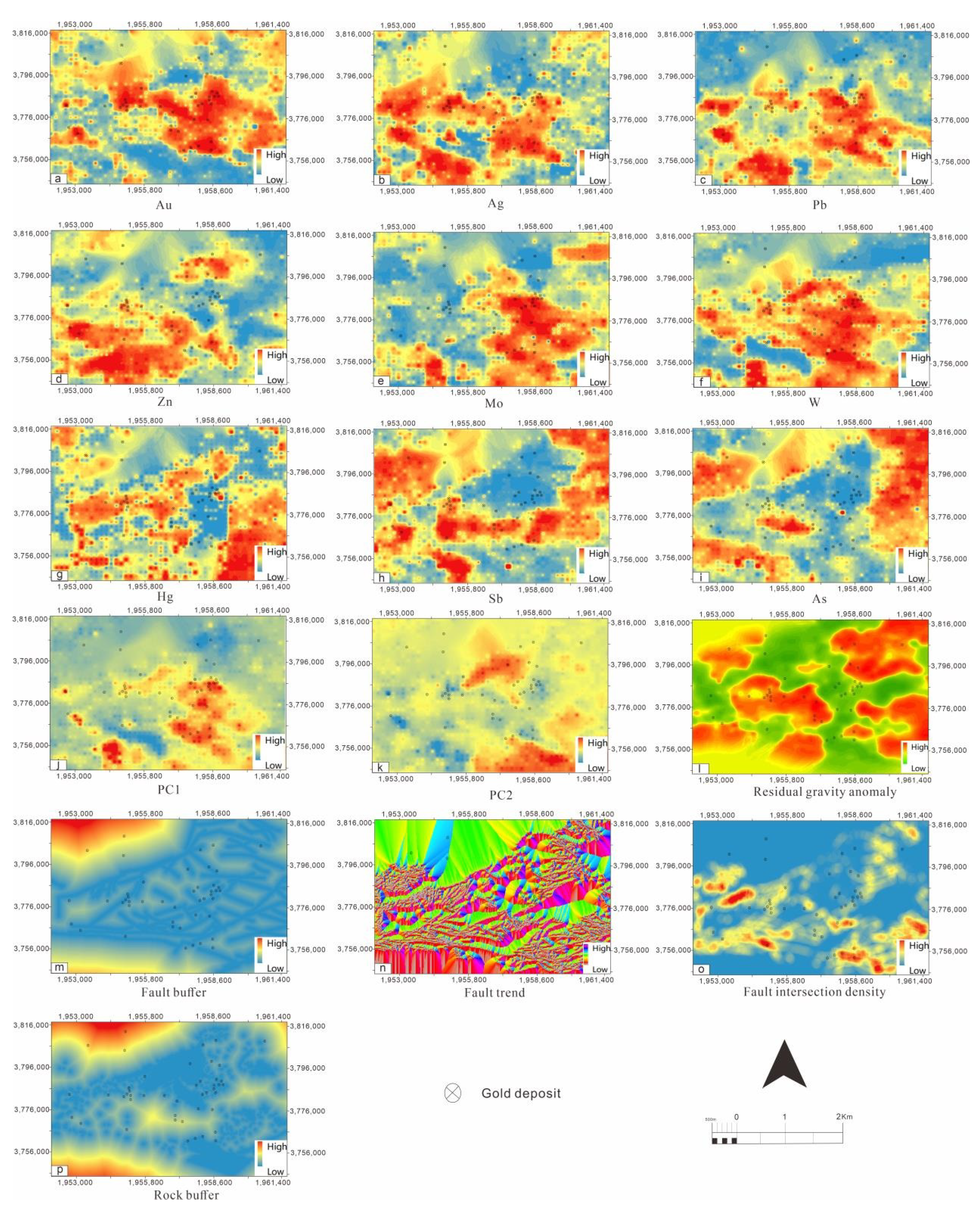
The source of ore-forming material provides the basis for the deposit formation [132,133]. A large number of studies on fluid inclusions and stable isotopes (O, H, C) in the Xiong ‘ershan area, show that the main metallogenic mechanism of gold deposits is fluid boiling, and the source of ore-forming fluids is mainly deep source materials [134,135,136,137,138]. The large-scale tectonic-magmatic-metallogenetic thermal event in the Early Cretaceous is characterized by the widespread exposure of faults and granitic batholiths in the study area (Figure 2). Granite batholith provides a heat source for the formation of gold and molybdenum deposits; therefore, the contemporaneous granite base in the region can be used as an important prediction factor. Reasonable estimation of the influence distance between granite rock mass and gold deposits indicates the positioning function for metallogenic prediction. Here, we analyzed the buffer distance layer by the distribution histogram (Figure 3) as one of the prediction factors. It showed the relationship between the granite rock mass (GRB) and ore-occurrence (Figure 4p). The granite intrusions usually exhibit low and gentle gravity anomalies owing to their low density. Figure 4l shows that the low gravity is roughly consistent with granitic intrusions, and the outline of several huge granitic intrusions can be recognized. The residual gravity anomaly (RGA) can highlight concealed granite geological bodies. We adopted the RGA as another prediction factor for MPM in the Xiong’ershan area.
Figure 2. Metallogenic model map of Xiong’er shan gold district: (a) Late Mesozoic tectonic-magmatic evolution scenario in Xiong’er shan Area; and (b) metallogenic model for the Au polymetallic deposits in Xiong’ershan Area (Modified after [139,140]).
Minerals 12 01621 g002

3.2.2. Transport and Deposition

Most gold deposits are hosted in faults. The ore-bearing faults in the study area are mainly NE and NWW faults, and a few are NW faults (i.e., Mao Chaoying fault). The Mao Chaoying fault zone is a deep fault that acted as pathways for the upward flow of deep-seated fluids (Figure 2b). The thick ore bodies (such as Qianhe and Hongzhuang gold deposits) are common in the intersection of NWW and NE faults in the Xiong’ershan area. Therefore, the fault buffer zone (FB), the European direction of the fault (FT), and the fault intersection density (FID) were selected as the prediction factor layers (Figure 4m–o).
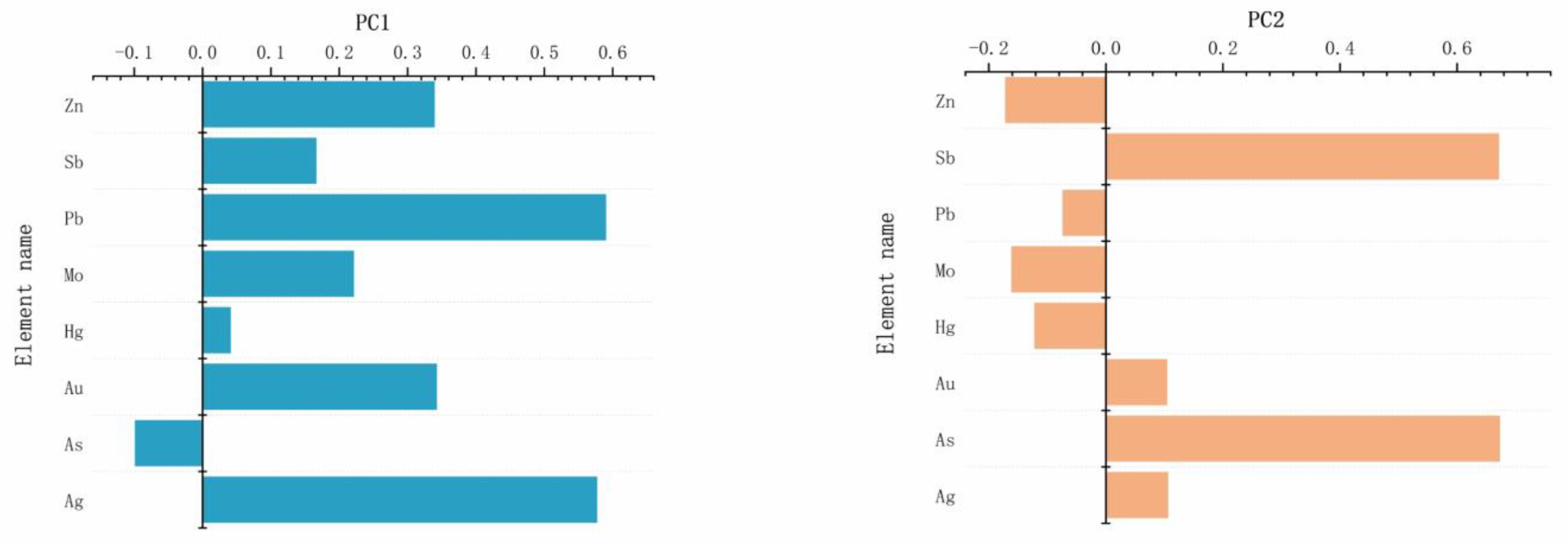
Stream sediment geochemical data can reveal regional to district-scale patterns associated with Au mineralization in the study area. We adopted the geochemical anomalies of Au, Ag, Pb, Zn, As, Sb, Hg, W and Mo, associated with fault-controlled mineralization on a regional scale (Figure 4a–k). In addition, considering the compositional nature of geochemical data (i.e., to address the constant sum problem existing in compositional data), we applied centered log-ratio transformation (clr) prior principal component analysis (PCA) [141,142,143]. Figure 5 shows the positive loading for Zn, Sb, Pb, Mo, Hg, Au and Ag elements, and the negative loading for As in the first principal component (PC1), where the Ag and Pb had a positive high factor load. This indicated that the high-value area of PC1 is more closely related to Ag, and Pb metallogenetic elements. Where Sb, Au, As, and Ag had a positive loading for the second principal component (PC2), the As and Sb as the front elements had a positive high factor load, and the high-value area was consistent with the low-value of PC2. This indicated that the low-value area of PC2 had great metallogenic potential.
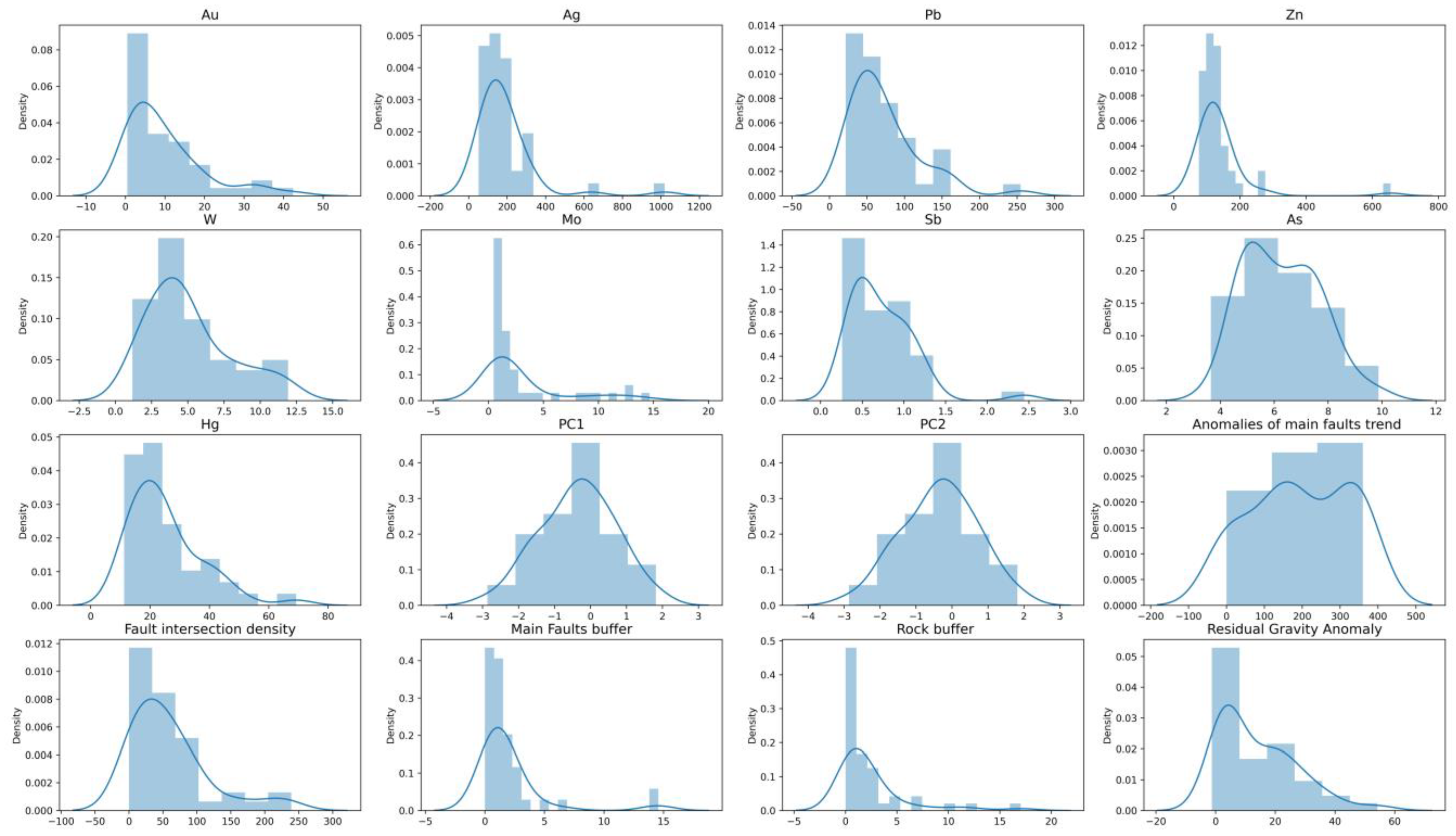
Therefore, the distribution histogram was used for the statistical analysis of the quantitative prediction factor as shown in Figure 3, along with the sixteen evidence maps derived by the prediction factor layers, which have been processed using a grid with a pixel size 130 m × 130 m (Figure 4).

3.2.3. Training and Validation Data

In this paper, 45 gold deposits developed in the study area were used as the training set, and each gold deposit includes 16 prediction variables (such as Au, Ag, Pb, Zn, Mo, W, Hg, Sb, As, PC1, PC2, RGA, FB, FT, FID, RB). The classification for MLA has a common basic assumption: the number of positive and negative datasets (samples) should be balanced [144,145]. If the positive and negative datasets are extremely imbalanced, the predicted results may be biased towards the majority classes with a large number of datasets [146,147]. Mineralization is a rare event, resulting in an insufficient number of training samples by MLA, and the number of deposits (positive samples) and non-deposits (negative samples) is not equal. In this paper, we used the synthetic minority over-sampling technique (SMOTE) based on geological knowledge constraints to balance data. The specific process is as follows: (1) based on the data of 45 known Au deposits (including 16 features) in the Xiong’ershan area and constrained by the optimal fault buffer radius of 3 km (Figure 3), yielded 945 SMOTE-augmented positive samples in the optimal ore-controlling adjacent area; (2) A total of 900 SMOTE-augmented negative samples were randomly selected from outside the 3 km threshold range of the non-anomalous area; (3) The knowledge-driven SMOTE datasets (generated by the (1) and (2)) are called MS (with the 945 deposits/positive and the 940 non-deposits/negative datasets) as the first datasets. The second datasets (denoted hereafter as OS datasets) were composited with 90 datasets (with the original known 45 deposits, 45 non-deposits are randomly selected non-mineralized locations)l (4) Then, we used the sixteen derived evidence maps, and the optimal threshold was used to show the Kernel density estimation curve (Figure 3) needed to accomplish the metallogenic predictionl (5) Finally, the dataset (with OS and MS) was divided into a test set and a train set (ratio of 2:8), and the test set was used to evaluate the accuracy and robustness of the model.

4. Results and Discussion

4.1. Parameters Optimization

Based on the Section 2.3 hyperparametric optimization process, the initially selected parameter space and the final reduced parameter space are shown in Table 3.
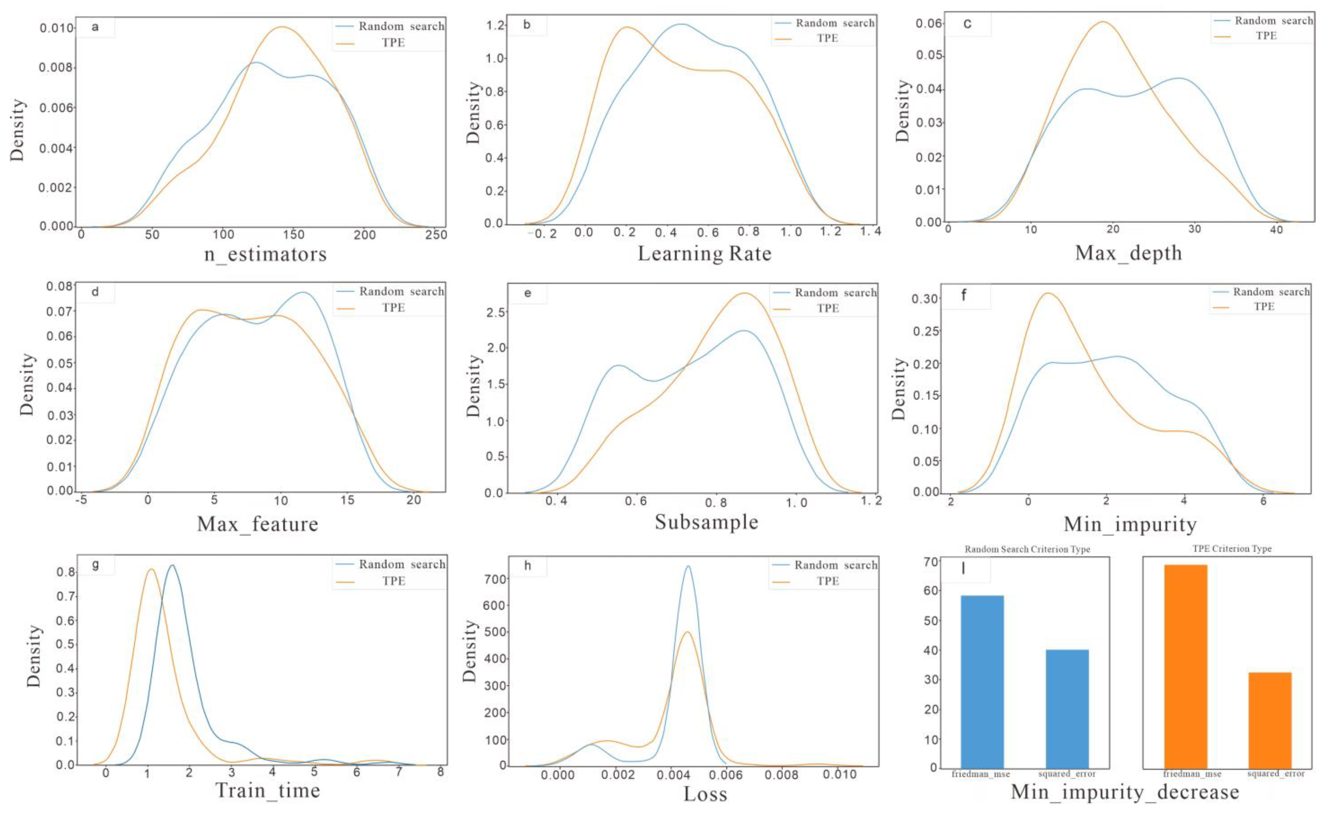
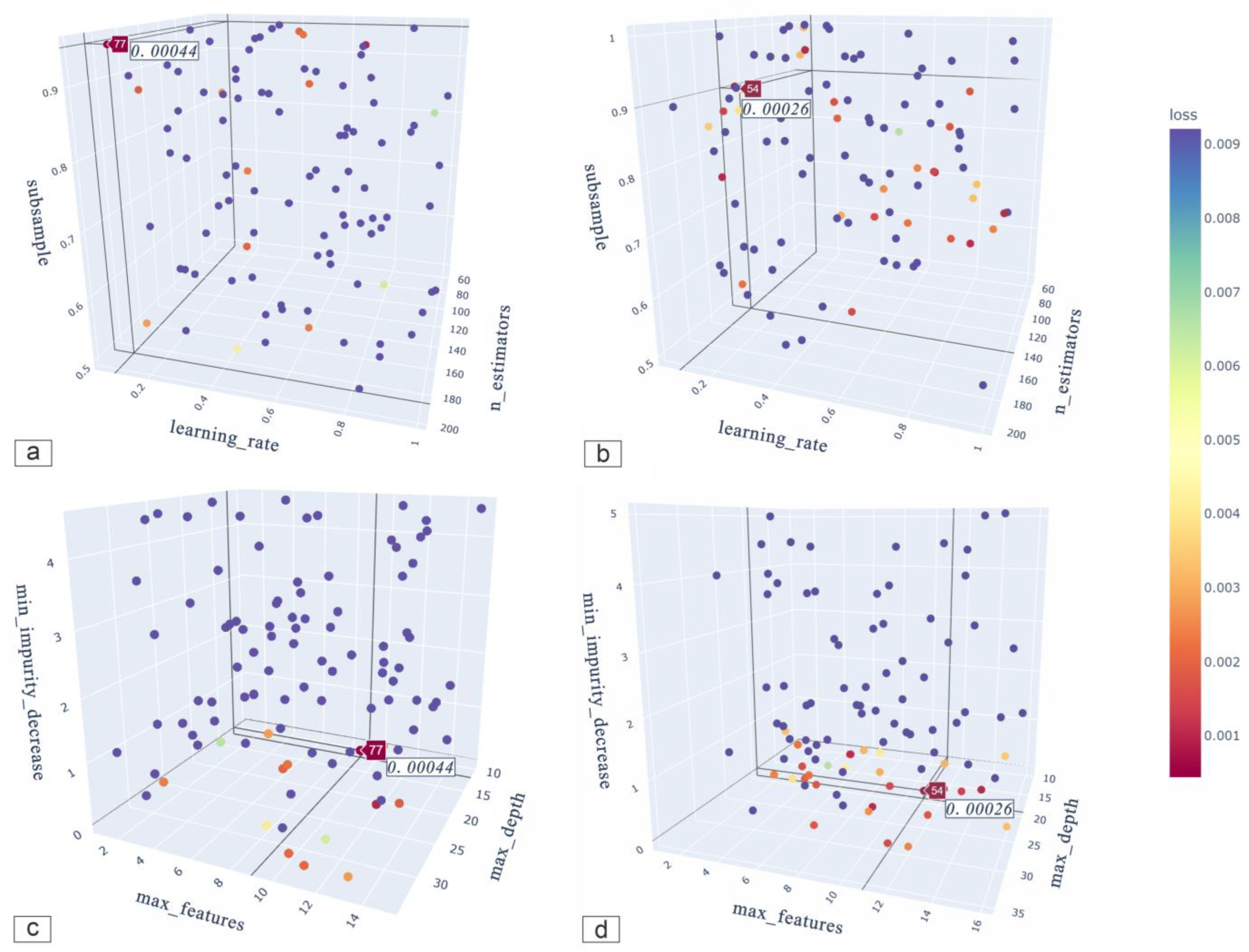
In order to compare and verify the performance of the two hyperparameter optimization algorithms on the final classification model, we plotted the kernel density estimates curve to understand the distribution of hyperparameters in both algorithms. Figure 6a–h shows that the distribution density curves of two hyperparameter optimization algorithms are consistent in the same domain space. It indicates that the hyperparameter distribution of the two algorithms is basically consistent. However, TPE tends to concentrate near the high-density area (placing more probabilities), resulting in the minimum loss in cross-validation. Figure 6i shows that the parameters criterion is mainly “friedman_mse”in random search and TPE-GBDT model. For pruning parameters “max_depth”, ”min_impurity_decrease” TPE has relatively lower values. Figure 7 shows that the value of the loss function is related to the spatial relationship based on the iterative process and the weak estimators. The random search reached the minimum loss function value at 77 iterations, while TPE reached the minimum loss function value at 54 iterations. Figure 6g also verified that in the same domain control interval, the training time of TPE was lower than that of the random search. The aforementioned results indirectly prove that the core idea of TPE is to spend more time evaluating promising hyperparametric values (i.e., the minimum loss function value). The loss value decreases with the increase of “learning rate” and “max_feature” (Figure 7b,d). The subsample and the “max_depth” shows a low loss value between 0.8–0.95, 15–25, respectively (Figure 7a,c). There is no obvious monotonic relation between the “min_impurity_decrease” parameter and loss value in the Xiong’ershan dataset. Compared with random search and TPE, the latter has a less objective function evaluation and better generalization performance on test sets. The optimal hyperparameters determined by the minimum loss function are shown in Table 4.

4.2. Performance Evaluation

Model evaluation plays a vital role in machine learning models. It helps to find the best model to represent our data. Different types of models (regression model and classification model) have different evaluation indexes. The evaluation indexes of the regression model include mean absolute error (MAE), mean square error (MSE), root mean square error (RMSE), and Coefficient of determination (R2) etc. The evaluation methods commonly used for classification models include k-fold cross validation to verify the model fitting effect, accuracy, recall rate and AUC index to evaluate the model generalization ability [148,149,150,151]. In our study, we selected the five-fold cross-validation, confusion matrix and the AUC as the performance evaluation for the GBDT model.
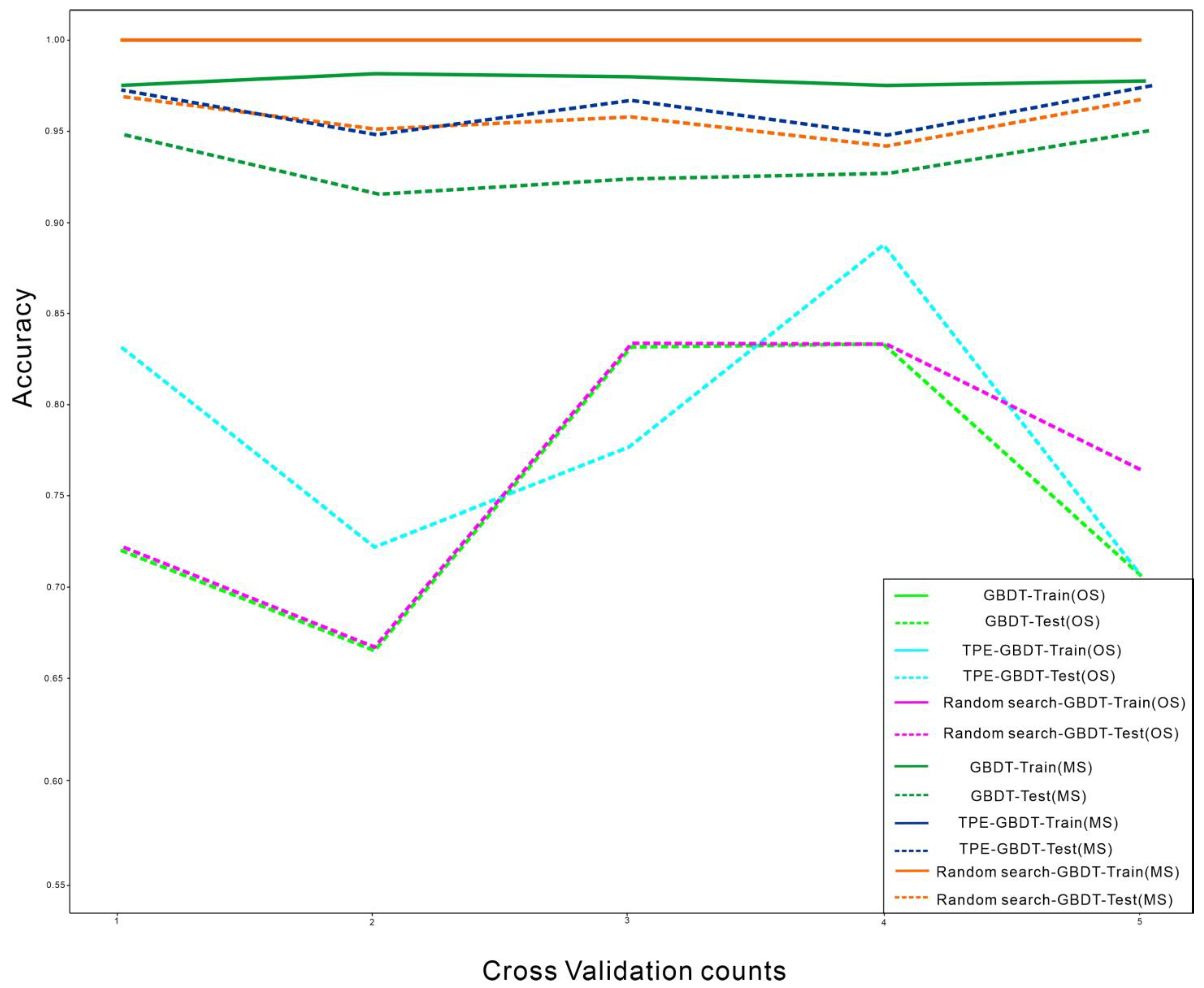
The five-fold cross-validation refers to roughly dividing the datasets into five parts, one of which is reserved for the validation model; the other samples are used for training. Cross-validation is repeated five times, with each sub-sample verified iterately. The results of an average of five times or other combination methods are used to finally obtain a single estimation. In this way, the model is more accurate. The GBDT model was trained according to the hyperparameters in Table 4, and the average accuracy of the five-fold cross-validation results obtained based on random search and TPE on the MS test set was 0.963 and 0.966, and on the OS test set was 0.764 and 0.786, respectively. This showed that the augmented datasets of the MS and the parameter adjustment improved the accuracy of the GBDT model (detail shows in Table 5). The results of the random search and TPE hyperparameter optimization were compared and analyzed after the five-fold cross-validation. Figure 8 shows that the results based on TPE had the best anti-overfitting effect for the GBDT model with the higher accuracy compared with the test sets.
The confusion matrix is a situation analysis table that summarizes the prediction results of the classification model in MLA. In the form of the matrix, records in datasets are summarized according to two criteria: the real category and the prediction category. The rows of the matrix represent the real value, and the columns of the matrix represent the predicted value.
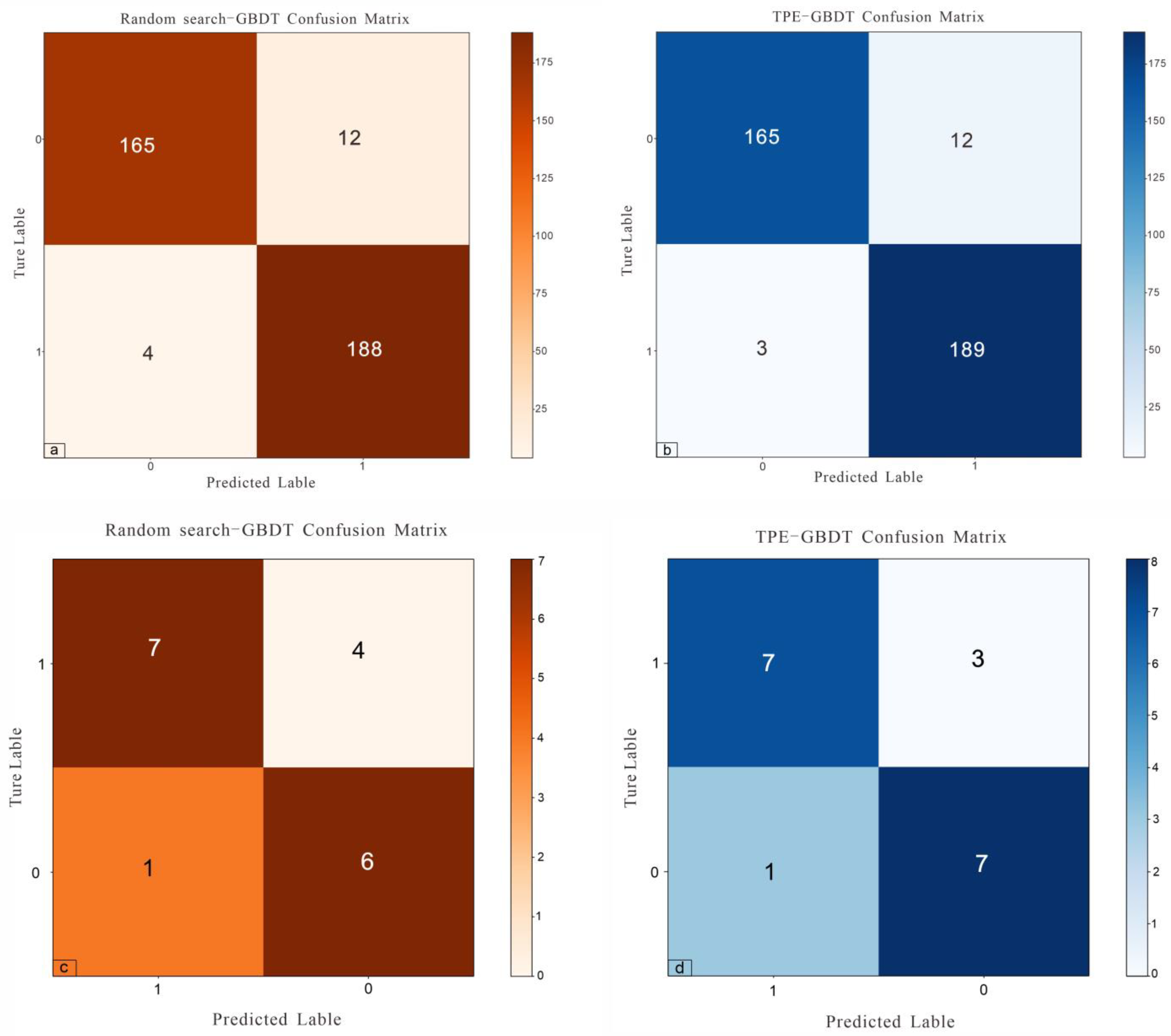
This mainly includes the real value being negative that is composed of the TP (true positive) and FN (false negative), and the real value being positive that is composed of the TN (true negative) and FP (false positive). The model’s generalization ability was analyzed and verified by the test sets (20% of the total training data), and it selected 369 data from the MS and 18 from OS datasets. Figure 9a,b shows that the random search-GBDT model and TPE-GBDT model have the same performance when the real value is negative with the MS datasets, as TN = 165, FP = 12, and a slightly different performance when the real value is positive, as FN = 3, TP = 189 in the TPE-GBDT model, that is, three of the positive samples were incorrectly predicted in this model, while the four of positive samples were incorrectly predicted in the Random search-GBDT model. Figure 9c,d shows that with the OS datasets, the random search-GBDT model and TPE-GBDT model had the same TP and FP. However, the FN with the TPE-GBDT model was lower than the random search-GBDT model, and the TN with the TPE-GBDT model was the opposite. According to the confusion matrix value, the secondary indicators (i.e., accuracy, recall, specificity) can be calculated to evaluate the model. Table 6 shows that Accuracy = 0.9593, recall = 0.984, and Precision = 0.941 with the TPE-GBDT model with the MS datasets. The values were slightly higher than the random search-GBDT model, indicating that the TPE-GBDT model performed better than the random search-GBDT model.
Another indicator to evaluate the performance of overall classification of the model is the ROC curve and the AUC value. The ROC (short for Receiver Operating Characteristic) is a curve in two-dimensional plane space. The AUC is the calculation result of the area under the ROC curve, which is a specific value. For any model, the closer the ROC curve is to the upper left, the larger the area is under the ROC curve, and the better the classification performance of the model. Figure 10 shows that ROC curve with the MS datasets all in the upper left corner; the AUC values of the TPE-GBDT model and random search-GBDT model were 0.985 and 0.981, respectively.

4.3. Mapping of Mineral Prospectivity

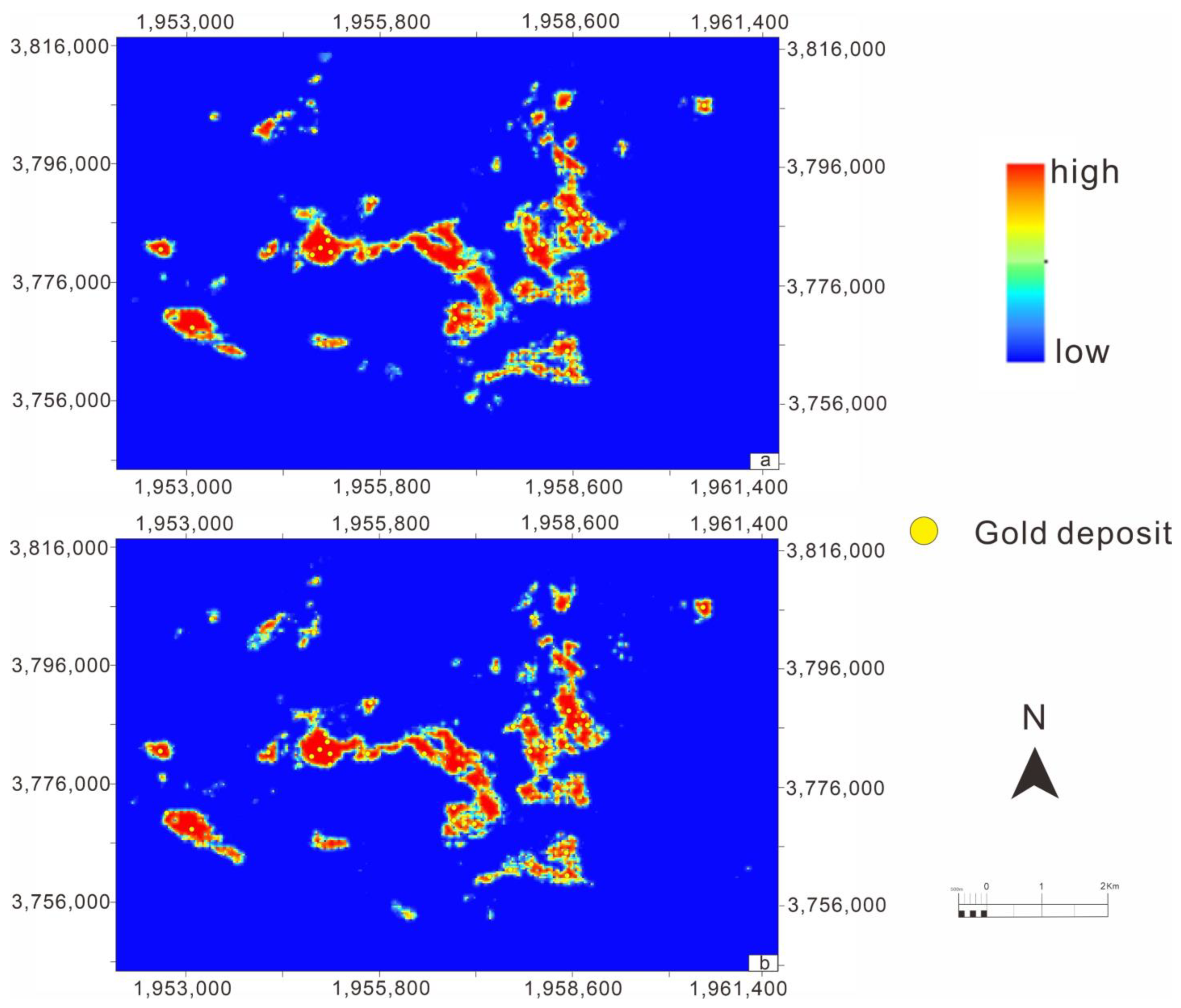
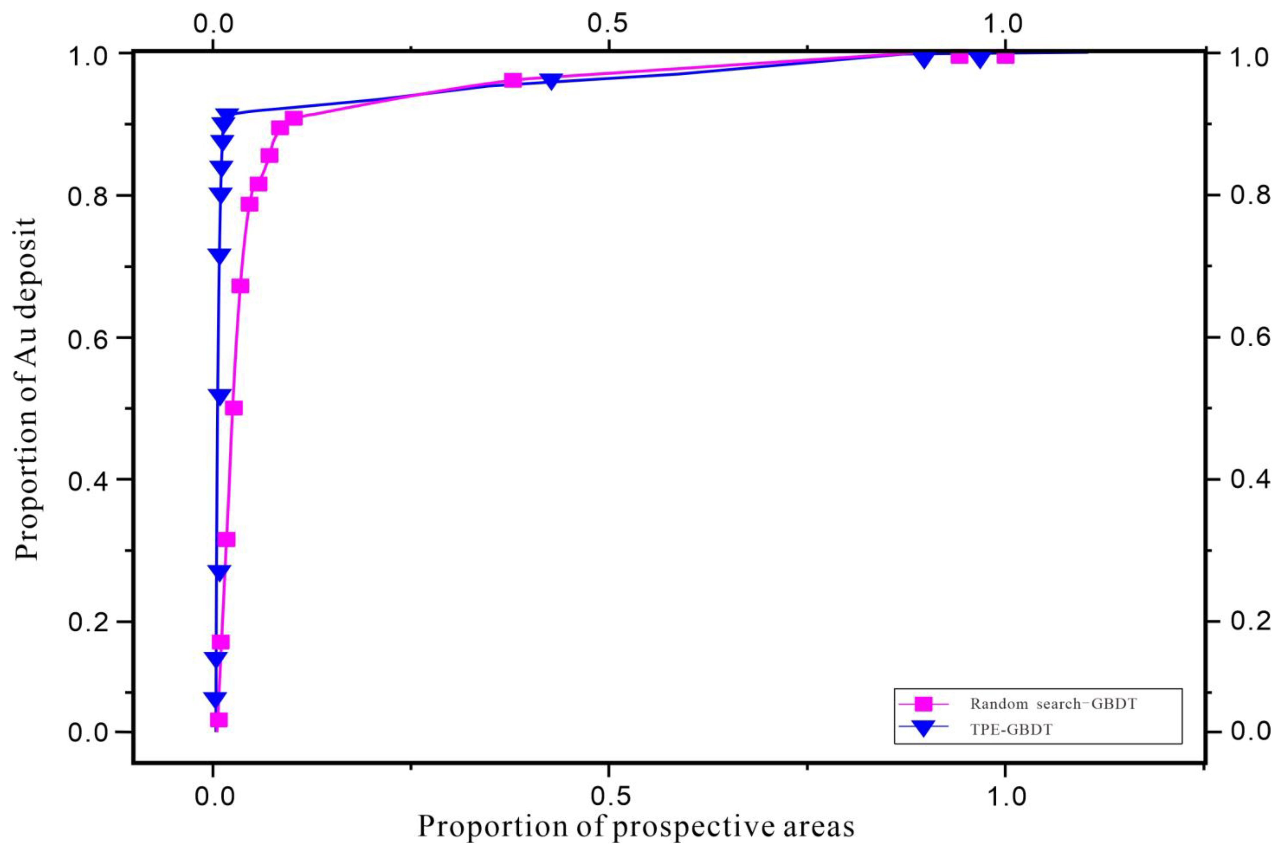
The MPM of the Xiong’ershan area using ArcGIS software was finally obtained through the above hyperparameter determination and model evaluation. The evaluation of prospectivity models with continuous probabilities (ranging from 0–1) of random search-GBDT (Figure 11a) and TPE-GBDT (Figure 11b) was conducted by measuring the correlation between the prospectivity values and known mineral occurrences, and for each model, the success-rate curves were plotted. The success-rate curve is a capture efficiency curve that indicates the relationship between the probability distribution and Au deposit locations. Figure 12 shows the proportion of the known gold deposits according to different percentages of prospective areas. It can be observed that the random search-GBDT and TPE-GBDT start from a similar success-rate curve, although the slope of the success-rate curve is steeper in the TPE-GBDT model, indicating that the TPE improved the performance of the GBDT predictive modeling.
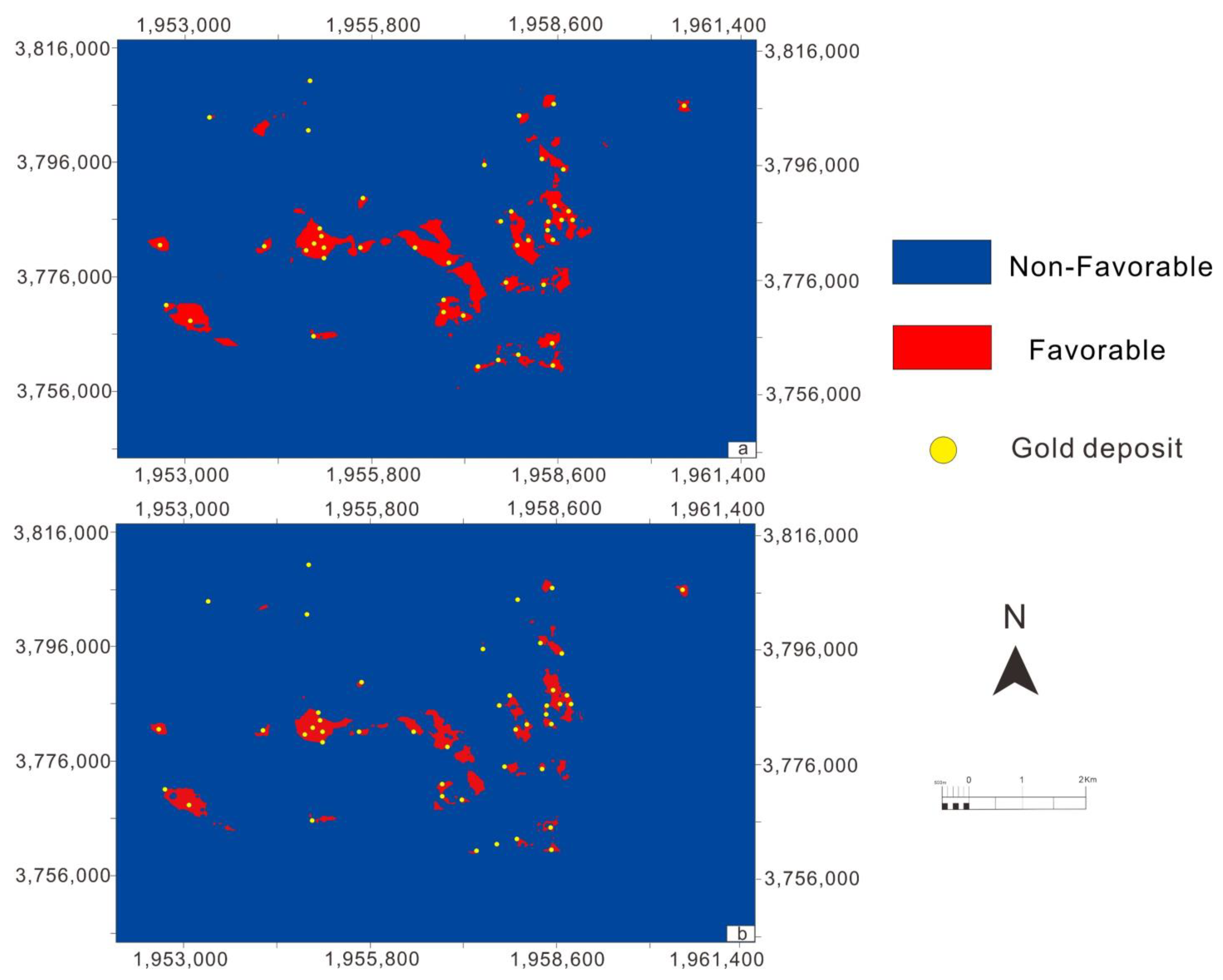
Then combined with the fact that the high probability part of the Random search-GBDT and TPE-GBDT models occupy 25% of the total study area. However thisthis 25% study area contains more than 93% of the known gold deposits (Figure 12). Finally, in order to delineate high-favorable targets in the study area. The cut-off values of Youden index in the ROC curve were adopted to discretize the TPE-GBDT and random search-GBDT predictive models, with the thresholds of 0.9211 and 0.7371, divided the prospectivity map of TPE-GBDT and Random search models into high potential (favorable) and low potential (non-favorable) areas, respectively. The highly favorable areas in the TPE-GBDT model (Figure 13b) captured 91% of known Au deposits within only 10.22% of the Xiong’er shan area, while the highly favorable areas of the Random search-GBDT model (Figure 13a) contained the same percentage of known Au occurrences but within larger areas (16.84%). Results suggested that the TPE-GBDT model is more consistent with the actual geological conditions, and more suitable for the next step of the exploration work.

5. Conclusions

In this study, we proposed a new method of TPE-GBDT generating MPM, which solved the problem of hyperparametric optimization in MLA. To some extent, it improved the accuracy of the MPM. The summary includes the following points:
(1) In view of the data imbalance of geological datasets, we used the knowledge-driven SMOTE method for data augmentation (as the MS datasets), which reached the balance of positive and negative sets, and then compared and analyzed these with the OS datasets (original 45 ore occurrence and the randomly selected 45 non-ore occurrence datasets), showing that it improved the precision and increased the interpretability of the model;
(2) The comprehensive AUC value and the accuracy of the models indicated that the GBDT models suit small data (insufficient known mineral deposits) training. The proposed random search-GBDT model and the TPE-GBDT model were able to adjust the GBDT for HPO automatically, and the AUC value was higher than that in the conventional GBDT, indicating that the HPO increased GBDT model accuracy;
(3) The spatial distribution of the random search-GBDT model and the TPE-GBDT model predicted results was consistent. A comparison with known Au deposits indicated that the TPE-GBDT model required less training time and had a more reasonable probability distribution than the random search-GBDT model. Thus, TPE-GBDT modeling can further reduce the uncertainty of predictions and enhance the predictive accuracy of mineral exploration.

Author Contributions

M.F.: Writing original draft, Data curation, Investigation, Methodology. K.X.: Supervision, Funding acquisition. L.S.: Data curation, Funding acquisition. S.Z.: Writing—review & editing. Y.X.: Visualization, Investigation. All authors have read and agreed to the published version of the manuscript.

Funding

This research was supported by the National Key R&D Program of China (Grant No. 2016YFC0600504).

Data Availability Statement

Not applicable.

Conflicts of Interest

The authors declare no conflict of interest.

References

  1. Payne, C.E.; Cunningham, F.; Peters, K.J.; Nielsen, S.; Puccioni, E.; Wildman, C.; Partington, G.A. From 2D to 3D: Prospectivity modelling in the Taupo volcanic zone, New Zealand. Ore Geol. Rev. 2015, 71, 558–577. [Google Scholar] [CrossRef]
  2. Zhang, Z.; Zhang, J.; Wang, G.; Carranza, E.J.M.; Pang, Z.; Wang, H. From 2D to 3D modeling of mineral prospectivity using multi-source geoscience datasets, Wulong Gold District, China. Nat. Resour. Res. 2020, 29, 345–364. [Google Scholar] [CrossRef]
  3. Joly, A.; Porwal, A.; McCuaig, T.C.; Chudasama, B.; Dentith, M.C.; Aitken, A.R. Mineral systems approach applied to GIS-based 2D-prospectivity modelling of geological regions: Insights from Western Australia. Ore Geol. Rev. 2015, 71, 673–702. [Google Scholar] [CrossRef]
  4. Yousefi, M.; Carranza, E.J.M. Prediction–area (P–A) plot and C–A fractal analysis to classify and evaluate evidential maps for mineral prospectivity modeling. Comput. Geosci. 2015, 79, 69–81. [Google Scholar] [CrossRef]
  5. Jiang, W.; Korsch, R.J.; Doublier, M.P.; Duan, J.; Costelloe, R. Mapping deep electrical conductivity structure in the mount isa region, northern australia: Implications for mineral prospectivity. J. Geophys. Res. Solid Earth 2019, 124, 10655–10671. [Google Scholar] [CrossRef] [Green Version]
  6. Li, T.; Zuo, R.; Xiong, Y.; Peng, Y. Random-drop data augmentation of deep convolutional neural network for mineral prospectivity mapping. Nat. Resour. Res. 2021, 30, 27–38. [Google Scholar] [CrossRef]
  7. Yang, N.; Zhang, Z.; Yang, J.; Hong, Z.; Shi, J. A convolutional neural network of GoogLeNet applied in mineral prospectivity prediction based on multi-source geoinformation. Nat. Resour. Res. 2021, 30, 3905–3923. [Google Scholar] [CrossRef]
  8. Wang, Z.; Zuo, R. Mineral prospectivity mapping using a joint singularity-based weighting method and long short-term memory network. Comput. Geosci. 2022, 158, 104974. [Google Scholar] [CrossRef]
  9. Xiao, K.; Li, N.; Porwal, A.; Holden, E.J.; Bagas, L.; Lu, Y. GIS-based 3D prospectivity mapping: A case study of Jiama copper-polymetallic deposit in Tibet, China. Ore Geol. Rev. 2015, 71, 611–632. [Google Scholar] [CrossRef]
  10. Li, X.; Yuan, F.; Zhang, M.; Jia, C.; Jowitt, S.M.; Ord, A.; Zheng, T.; Hu, X.; Li, Y. Three-dimensional mineral prospectivity modeling for targeting of concealed mineralization within the Zhonggu iron orefield, Ningwu Basin, China. Ore Geol. Rev. 2015, 71, 633–654. [Google Scholar] [CrossRef]
  11. Li, X.; Yuan, F.; Zhang, M.; Jowitt, S.M.; Ord, A.; Zhou, T.; Dai, W. 3D computational simulation-based mineral prospectivity modeling for exploration for concealed Fe–Cu skarn-type mineralization within the Yueshan orefield, Anqing district, Anhui Province, China. Ore Geol. Rev. 2019, 105, 1–17. [Google Scholar] [CrossRef]
  12. Xiang, J.; Xiao, K.; Carranza, E.J.M.; Chen, J.; Li, S. 3D mineral prospectivity mapping with random forests: A case study of Tongling, Anhui, China. Nat. Resour. Res. 2020, 29, 395–414. [Google Scholar] [CrossRef]
  13. Mao, X.; Zhang, W.; Liu, Z.; Ren, J.; Bayless, R.C.; Deng, H. 3D mineral prospectivity modeling for the low-sulfidation epithermal gold deposit: A case study of the axi gold deposit, western Tianshan, NW China. Minerals 2020, 10, 233. [Google Scholar] [CrossRef] [Green Version]
  14. Qin, Y.; Liu, L.; Wu, W. Machine learning-based 3D modeling of mineral prospectivity mapping in the Anqing Orefield, Eastern China. Nat. Resour. Res. 2021, 30, 3099–3120. [Google Scholar] [CrossRef]
  15. Mohammadpour, M.; Bahroudi, A.; Abedi, M. Three dimensional mineral prospectivity modeling by evidential belief functions, a case study from Kahang porphyry Cu deposit. J. Afr. Earth Sci. 2021, 174, 104098. [Google Scholar] [CrossRef]
  16. Xiao, K.; Xiang, J.; Fan, M.; Xu, Y. 3D mineral prospectivity mapping based on deep metallogenic prediction theory: A case study of the Lala Copper Mine, Sichuan, China. J. Earth Sci. 2021, 32, 348–357. [Google Scholar] [CrossRef]
  17. Porwal, A.; Carranza, E.J.M.; Hale, M. Knowledge-driven and data-driven fuzzy models for predictive mineral potential mapping. Nat. Resour. Res. 2003, 12, 1–25. [Google Scholar] [CrossRef]
  18. Carranza, E.J.M.; Van Ruitenbeek, F.J.A.; Hecker, C.; van der Meijde, M.; van der Meer, F.D. Knowledge-guided data-driven evidential belief modeling of mineral prospectivity in Cabo de Gata, SE Spain. Int. J. Appl. Earth Obs. Geoinf. 2008, 10, 374–387. [Google Scholar] [CrossRef]
  19. Abedi, M.; Torabi, S.A.; Norouzi, G.H.; Hamzeh, M. ELECTRE III: A knowledge-driven method for integration of geophysical data with geological and geochemical data in mineral prospectivity mapping. J. Appl. Geophys. 2012, 87, 9–18. [Google Scholar] [CrossRef]
  20. Harris, J.R.; Grunsky, E.; Behnia, P.; Corrigan, D. Data-and knowledge-driven mineral prospectivity maps for Canada’s North. Ore Geol. Rev. 2015, 71, 788–803. [Google Scholar] [CrossRef]
  21. Hosseini, S.A.; Abedi, M. Data envelopment analysis: A knowledge-driven method for mineral prospectivity mapping. Comput. Geosci. 2015, 82, 111–119. [Google Scholar] [CrossRef]
  22. Abedi, M.; Kashani, S.B.M.; Norouzi, G.H.; Yousefi, M. A deposit scale mineral prospectivity analysis: A comparison of various knowledge-driven approaches for porphyry copper targeting in Seridune, Iran. J. Afr. Earth Sci. 2017, 128, 127–146. [Google Scholar] [CrossRef]
  23. Skirrow, R.G.; Murr, J.; Schofield, A.; Huston, D.L.; van der Wielen, S.; Czarnota, K.; Coghlan, R.; Highet, L.M.; Connolly, D.; Doublier, M.; et al. Mapping iron oxide Cu-Au (IOCG) mineral potential in Australia using a knowledge-driven mineral systems-based approach. Ore Geol. Rev. 2019, 113, 103011. [Google Scholar] [CrossRef]
  24. Daviran, M.; Parsa, M.; Maghsoudi, A.; Ghezelbash, R. Quantifying uncertainties linked to the diversity of mathematical frameworks in knowledge-driven mineral prospectivity mapping. Nat. Resour. Res. 2022, 31, 2271–2287. [Google Scholar] [CrossRef]
  25. Carranza, E.J.M.; Hale, M.; Faassen, C. Selection of coherent deposit-type locations and their application in data-driven mineral prospectivity mapping. Ore Geol. Rev. 2008, 33, 536–558. [Google Scholar] [CrossRef]
  26. Carranza, E.J.M. Objective selection of suitable unit cell size in data-driven modeling of mineral prospectivity. Comput. Geosci. 2009, 35, 2032–2046. [Google Scholar] [CrossRef]
  27. Carranza, E.J.M.; Laborte, A.G. Data-driven predictive mapping of gold prospectivity, Baguio district, Philippines: Application of Random Forests algorithm. Ore Geol. Rev. 2015, 71, 777–787. [Google Scholar] [CrossRef]
  28. Carranza, E.J.M.; Laborte, A.G. Data-driven predictive modeling of mineral prospectivity using random forests: A case study in Catanduanes Island (Philippines). Nat. Resour. Res. 2016, 25, 35–50. [Google Scholar] [CrossRef]
  29. Yousefi, M.; Nykänen, V. Data-driven logistic-based weighting of geochemical and geological evidence layers in mineral prospectivity mapping. J. Geochem. Explor. 2016, 164, 94–106. [Google Scholar] [CrossRef]
  30. Yousefi, M.; Carranza, E.J.M. Data-driven index overlay and Boolean logic mineral prospectivity modeling in greenfields exploration. Nat. Resour. Res. 2016, 25, 3–18. [Google Scholar] [CrossRef]
  31. McKay, G.; Harris, J.R. Comparison of the data-driven random forests model and a knowledge-driven method for mineral prospectivity mapping: A case study for gold deposits around the Huritz Group and Nueltin Suite, Nunavut, Canada. Nat. Resour. Res. 2016, 25, 125–143. [Google Scholar] [CrossRef]
  32. Chen, Y.; Wu, W. Isolation forest as an alternative data-driven mineral prospectivity mapping method with a higher data-processing efficiency. Nat. Resour. Res. 2019, 28, 31–46. [Google Scholar] [CrossRef]
  33. Sun, T.; Li, H.; Wu, K.; Chen, F.; Zhu, Z.; Hu, Z. Data-driven predictive modelling of mineral prospectivity using machine learning and deep learning methods: A case study from southern Jiangxi Province, China. Minerals 2020, 10, 102. [Google Scholar] [CrossRef] [Green Version]
  34. Zhang, S.; Carranza, E.J.M.; Wei, H.; Xiao, K.; Yang, F.; Xiang, J.; Zhang, S.; Xu, Y. Data-driven Mineral Prospectivity Mapping by Joint Application of Unsupervised Convolutional Auto-encoder Network and Supervised Convolutional Neural Network. Nat. Resour. Res. 2021, 30, 1011–1031. [Google Scholar] [CrossRef]
  35. Parsa, M.; Carranza, E.J.M. Modulating the impacts of stochastic uncertainties linked to deposit locations in data-driven predictive mapping of mineral prospectivity. Nat. Resour. Res. 2021, 30, 3081–3097. [Google Scholar] [CrossRef]
  36. Bacardit, J.; Llorà, X. Large scale data mining using genetics-based machine learning. In Proceedings of the 11th Annual Conference Companion on Genetic and Evolutionary Computation Conference, Montréal, Canada, 8–12 July 2009; pp. 3381–3412. [Google Scholar]
  37. Najafabadi, M.M.; Villanustre, F.; Khoshgoftaar, T.M.; Seliya, N.; Wald, R.; Muharemagic, E. Deep learning applications and challenges in big data analytics. J. Big Data 2015, 2, 1. [Google Scholar] [CrossRef] [Green Version]
  38. Angermueller, C.; Pärnamaa, T.; Parts, L.; Stegle, O. Deep learning for computational biology. Mol. Syst. Biol. 2016, 12, 878. [Google Scholar] [CrossRef]
  39. Sun, C.; Shrivastava, A.; Singh, S.; Gupta, A. Revisiting unreasonable effectiveness of data in deep learning era. In Proceedings of the IEEE International Conference on Computer Vision, Venice, Italy, 22–29 October 2017; pp. 843–852. [Google Scholar]
  40. Rusk, N. Deep learning. Nat. Methods 2016, 13, 35. [Google Scholar] [CrossRef]
  41. Nguyen, G.; Dlugolinsky, S.; Bobák, M.; Tran, V.; López García, Á.; Heredia, I.; Malík, P.; Hluchý, L. Machine learning and deep learning frameworks and libraries for large-scale data mining: A survey. Artif. Intell. Rev. 2019, 52, 77–124. [Google Scholar] [CrossRef] [Green Version]
  42. Zuo, R. Geodata science-based mineral prospectivity mapping: A review. Nat. Resour. Res. 2020, 29, 3415–3424. [Google Scholar] [CrossRef]
  43. Chawla, N.V.; Bowyer, K.W.; Hall, L.O.; Kegelmeyer, W.P. SMOTE: Synthetic minority over-sampling technique. J. Artif. Intell. Res. 2002, 16, 321–357. [Google Scholar] [CrossRef]
  44. Han, H.; Wang, W.Y.; Mao, B.H. Borderline-SMOTE: A new over-sampling method in imbalanced data sets learning. In Proceedings of the International Conference on Intelligent Computing, Hefei China, 23–26 August 2005; Springer: Berlin/Heidelberg, Germany, 2005; pp. 878–887. [Google Scholar]
  45. Bunkhumpornpat, C.; Sinapiromsaran, K.; Lursinsap, C. Safe-level-smote: Safe-level-synthetic minority over-sampling technique for handling the class imbalanced problem. In Proceedings of the Pacific-Asia Conference on Knowledge Discovery and Data Mining, Bangkok, Thailand, 27–30 April 2009; Springer: Berlin/Heidelberg, Germany, 2009; pp. 475–482. [Google Scholar]
  46. Bunkhumpornpat, C.; Sinapiromsaran, K.; Lursinsap, C. DBSMOTE: Density-based synthetic minority over-sampling technique. Appl. Intell. 2012, 36, 664–684. [Google Scholar] [CrossRef]
  47. Guzmán-Ponce, A.; Sánchez, J.S.; Valdovinos, R.M.; Marcial-Romero, J.R. DBIG-US: A two-stage under-sampling algorithm to face the class imbalance problem. Expert Syst. Appl. 2021, 168, 114301. [Google Scholar] [CrossRef]
  48. Soltanzadeh, P.; Hashemzadeh, M. RCSMOTE: Range-Controlled synthetic minority over-sampling technique for handling the class imbalance problem. Inf. Sci. 2021, 542, 92–111. [Google Scholar] [CrossRef]
  49. Peng, C.Y.; Park, Y.J. A New Hybrid Under-sampling Approach to Imbalanced Classification Problems. Appl. Artif. Intell. 2022, 36, 1975393. [Google Scholar] [CrossRef]
  50. Lenka, S.R.; Bisoy, S.K.; Priyadarshini, R.; Nayak, B. Representative-based cluster undersampling technique for imbalanced credit scoring datasets. In Innovations in Computational Intelligence and Computer Vision; Springer: Singapore, 2022; pp. 119–129. [Google Scholar]
  51. Amirruddin, A.D.; Muharam, F.M.; Ismail, M.H.; Tan, N.P.; Ismail, M.F. Synthetic Minority Over-sampling TEchnique (SMOTE) and Logistic Model Tree (LMT)-Adaptive Boosting algorithms for classifying imbalanced datasets of nutrient and chlorophyll sufficiency levels of oil palm (Elaeis guineensis) using spectroradiometers and unmanned aerial vehicles. Comput. Electron. Agric. 2022, 193, 106646. [Google Scholar]
  52. Perez, L.; Wang, J. The effectiveness of data augmentation in image classification using deep learning. arXiv 2017, arXiv:1712.04621. Preprint. [Google Scholar]
  53. Abbaszadeh, M.; Soltani-Mohammadi, S.; Ahmed, A.N. Optimization of support vector machine parameters in modeling of Iju deposit mineralization and alteration zones using particle swarm optimization algorithm and grid search method. Comput. Geosci. 2022, 165, 105140. [Google Scholar] [CrossRef]
  54. Shorten, C.; Khoshgoftaar, T.M. A survey on image data augmentation for deep learning. J. Big Data 2019, 6, 60. [Google Scholar] [CrossRef]
  55. Inoue, H. Data augmentation by pairing samples for images classification. arXiv 2018, arXiv:1801.02929; Preprint. [Google Scholar]
  56. Jackson, P.T.; Abarghouei, A.A.; Bonner, S.; Breckon, T.P.; Obara, B. Style augmentation: Data augmentation via style randomization. CVPR Workshops 2019, 6, 10–11. [Google Scholar]
  57. Raj, R.; Mathew, J.; Kannath, S.K.; Rajan, J. Crossover based technique for data augmentation. Comput. Methods Programs Biomed. 2022, 218, 106716. [Google Scholar] [CrossRef] [PubMed]
  58. Radford, A.; Metz, L.; Chintala, S. Unsupervised representation learning with deep convolutional generative adversarial networks. arXiv 2015, arXiv:1511.06434. Preprint. [Google Scholar]
  59. Creswell, A.; White, T.; Dumoulin, V.; Arulkumaran, K.; Sengupta, B.; Bharath, A.A. Generative adversarial networks: An overview. IEEE Signal Process. Mag. 2018, 35, 53–65. [Google Scholar] [CrossRef] [Green Version]
  60. Cubuk, E.D.; Zoph, B.; Mane, D.; Vasudevan, V.; Le, Q.V. Autoaugment: Learning augmentation policies from data. arXiv 2018, arXiv:1805.09501. Preprint. [Google Scholar]
  61. Lim, S.; Kim, I.; Kim, T.; Kim, C.; Kim, S. Fast autoaugment. Adv. Neural Inf. Process. Syst. 2019, 32, 1–11. [Google Scholar]
  62. Xiong, Y.; Zuo, R. Effects of misclassification costs on mapping mineral prospectivity. Ore Geol. Rev. 2017, 82, 1–9. [Google Scholar] [CrossRef]
  63. Xiong, Y.; Zuo, R. GIS-based rare events logistic regression for mineral prospectivity mapping. Comput. Geosci. 2018, 111, 18–25. [Google Scholar] [CrossRef]
  64. Lin, C.F.; Wang, S.D. Fuzzy support vector machines. IEEE Trans. Neural Netw. 2002, 13, 464–471. [Google Scholar]
  65. Min, R.; Cheng, H.D. Effective image retrieval using dominant color descriptor and fuzzy support vector machine. Pattern Recognit. 2009, 42, 147–157. [Google Scholar] [CrossRef]
  66. Batuwita, R.; Palade, V. FSVM-CIL: Fuzzy support vector machines for class imbalance learning. IEEE Trans. Fuzzy Syst. 2010, 18, 558–571. [Google Scholar] [CrossRef]
  67. Yu, H.; Sun, C.; Yang, X.; Zheng, S.; Zou, H. Fuzzy support vector machine with relative density information for classifying imbalanced data. IEEE Trans. Fuzzy Syst. 2019, 27, 2353–2367. [Google Scholar] [CrossRef]
  68. Maldonado, S.; López, J.; Vairetti, C. Time-weighted Fuzzy Support Vector Machines for classification in changing environments. Inf. Sci. 2021, 559, 97–110. [Google Scholar] [CrossRef]
  69. Yu, X.; Zhang, X. Imbalanced data classification algorithm based on hybrid model. In Proceedings of the International Conference on Machine Learning and Cybernetics, Xi’an, China, 15–17 July 2012; IEEE: New York, NY, USA, 2012; Volume 2, pp. 735–740. [Google Scholar]
  70. Zhang, M.; Wu, M. Efficient super greedy boosting for classification. In Proceedings of the 2020 10th Institute of Electrical and Electronics Engineers International Conference on Cyber Technology in Automation, Control, and Intelligent Systems (CYBER), Xi’an, China, 10–13 October 2020; IEEE: New York, NY, USA, 2020; pp. 192–197. [Google Scholar]
  71. Ding, J.; Wang, S.; Jia, L.; You, J.; Jiang, Y. Spark-based Ensemble Learning for Imbalanced Data Classification. Int. J. Perform. Eng. 2018, 14, 955. [Google Scholar] [CrossRef]
  72. Wang, Y.; Liao, X.; Lin, S. Rescaled boosting in classification. IEEE Trans. Neural Netw. Learn. Syst. 2019, 30, 2598–2610. [Google Scholar] [CrossRef]
  73. Lim, S.K.; Loo, Y.; Tran, N.T.; Cheung, N.M.; Roig, G.; Elovici, Y. Doping: Generative data augmentation for unsupervised anomaly detection with gan. In Proceedings of the 2018 IEEE International Conference on Data Mining (ICDM), Singapore, 17–20 November 2018; IEEE: New York, NY, USA, 2018; pp. 1122–1127. [Google Scholar]
  74. Wen, Q.; Sun, L.; Yang, F.; Song, X.; Gao, J.; Wang, X.; Xu, H. Time series data augmentation for deep learning: A survey. arXiv 2002, arXiv:2002.12478. Preprint. [Google Scholar]
  75. Al Olaimat, M.; Lee, D.; Kim, Y.; Kim, J.; Kim, J. A learning-based data augmentation for network anomaly detection. In Proceedings of the 2020 29th International Conference on Computer Communications and Networks (ICCCN), Honolulu, HI, USA, 3–6 August 2020; IEEE: New York, NY, USA, 2020; pp. 1–10. [Google Scholar]
  76. Sinha, A.; Ayush, K.; Song, J.; Uzkent, B.; Jin, H.; Ermon, S. Negative data augmentation. arXiv 2021, arXiv:2102.05113. Preprint. [Google Scholar]
  77. Chen, R.T.; Rubanova, Y.; Bettencourt, J.; Duvenaud, D.K. Neural ordinary differential equations. In Advances in Neural Information Processing Systems; NeurIPS: New Orleans, LA, USA, 2018; p. 31. [Google Scholar]
  78. Song, L.; Gong, D.; Li, Z.; Liu, C.; Liu, W. Occlusion robust face recognition based on mask learning with pairwise differential siamese network. In Proceedings of the IEEE/CVF International Conference on Computer Vision, Seould, Republic of Korea, 27 October–2 November 2019; pp. 773–782. [Google Scholar]
  79. Meldo, A.A.; Utkin, L.V. A new approach to differential lung diagnosis with ct scans based on the siamese neural network. J. Phys. 2019, 1236, 12–58. [Google Scholar] [CrossRef]
  80. Ruthotto, L.; Haber, E. Deep neural networks motivated by partial differential equations. J. Math. Imaging Vis. 2020, 62, 352–364. [Google Scholar] [CrossRef] [Green Version]
  81. Soleymani, S.; Chaudhary, B.; Dabouei, A.; Dawson, J.; Nasrabadi, N.M. Differential morphed face detection using deep siamese networks. In International Conference on Pattern Recognition; Springer: Cham, Switzerland, 2021; pp. 560–572. [Google Scholar]
  82. Booth, A.; Gerding, E.; McGroarty, F. Automated trading with performance weighted random forests and seasonality. Expert Syst. Appl. 2014, 41, 3651–3661. [Google Scholar] [CrossRef]
  83. Li, H.B.; Wang, W.; Ding, H.W.; Dong, J. Trees weighting random forest method for classifying high-dimensional noisy data. In Proceedings of the 2010 IEEE 7th International Conference on e-Business Engineering, Shanghai, China, 10–12 November 2010; IEEE: New York, NY, USA, 2010; pp. 160–163. [Google Scholar]
  84. Gajowniczek, K.; Grzegorczyk, I.; Ząbkowski, T.; Bajaj, C. Weighted random forests to improve arrhythmia classification. Electronics 2020, 9, 99. [Google Scholar] [CrossRef] [PubMed] [Green Version]
  85. Chowdhury, M.M.U.; Hammond, F.; Konowicz, G.; Xin, C.; Wu, H.; Li, J. A few-shot deep learning approach for improved intrusion detection. In Proceedings of the 2017 IEEE 8th Annual Ubiquitous Computing, Electronics and Mobile Communication Conference (UEMCON), New York, NY, USA, 19–21 October 2017; IEEE: New York, NY, USA, 2017; pp. 456–462. [Google Scholar]
  86. Wang, A.; Zhang, Y.; Wu, H.; Jiang, K.; Wang, M. Few-shot learning based balanced distribution adaptation for heterogeneous defect prediction. IEEE Access 2020, 8, 32989–33001. [Google Scholar] [CrossRef]
  87. Zhang, B.; Jiang, H.; Li, X.; Feng, S.; Ye, Y.; Ye, R. MetaDT: Meta Decision Tree for Interpretable Few-Shot Learning. arXiv 2022, arXiv:2203.01482. Preprint. [Google Scholar]
  88. Bishop, C.M. Model-based machine learning. Philosophical Trans. R. Soc. A Math. Phys. Eng. Sci. 2013, 371, 20120222. [Google Scholar] [CrossRef] [Green Version]
  89. Singh, A.; Thakur, N.; Sharma, A. A review of supervised machine learning algorithms. In Proceedings of the 2016 3rd International Conference on Computing for Sustainable Global Development (INDIACom), New Delhi, India, 16–18 March 2016; IEEE: New York, NY, USA, 2016; pp. 1310–1315. [Google Scholar]
  90. Kern, C.; Klausch, T.; Kreuter, F. Tree-based machine learning methods for survey research. Surv. Res. Methods 2019, 13, 73. [Google Scholar]
  91. Mahesh, B. Machine learning algorithms-a review. Int. J. Sci. Res. 2020, 9, 381–386. [Google Scholar]
  92. Charbuty, B.; Abdulazeez, A. Classification based on decision tree algorithm for machine learning. J. Appl. Sci. Technol. Trends 2021, 2, 20–28. [Google Scholar] [CrossRef]
  93. Flores, V.; Keith, B.; Leiva, C. Using artificial intelligence techniques to improve the prediction of copper recovery by leaching. J. Sens. 2020, 2020, 2454875. [Google Scholar] [CrossRef] [Green Version]
  94. Zou, Y.; Chen, Y.; Deng, H. Gradient boosting decision tree for lithology identification with well logs: A case study of zhaoxian gold deposit, shandong peninsula, China. Nat. Resour. Res. 2021, 30, 3197–3217. [Google Scholar] [CrossRef]
  95. Kotthoff, L.; Thornton, C.; Hoos, H.H.; Hutter, F.; Leyton-Brown, K. Auto-WEKA: Automatic model selection and hyperparameter optimization in WEKA. In Automated Machine Learning; Springer: Cham, Switzerland, 2019; pp. 81–95. [Google Scholar]
  96. Wong, J.; Manderson, T.; Abrahamowicz, M.; Buckeridge, D.L.; Tamblyn, R. Can hyperparameter tuning improve the performance of a super learner? A case study. Epidemiology 2019, 30, 521. [Google Scholar] [CrossRef]
  97. Rafique, D.; Velasco, L. Machine Learning for Network Automation: Overview, Architecture, and Applications [Invited Tutorial]. J. Opt. Commun. Netw. 2018, 10, D126–D143. [Google Scholar] [CrossRef] [Green Version]
  98. Marshall, I.J.; Wallace, B.C. Toward systematic review automation: A practical guide to using machine learning tools in research synthesis. Syst. Rev. 2019, 8, 163. [Google Scholar] [CrossRef] [PubMed]
  99. Wang, W.; Siau, K. Artificial intelligence, machine learning, automation, robotics, future of work and future of humanity: A review and research agenda. J. Database Manag. 2019, 30, 61–79. [Google Scholar] [CrossRef]
  100. Bergstra, J.; Bardenet, R.; Bengio, Y.; Kégl, B. Algorithms for hyper-parameter optimization. Adv. Neural Inf. Process. Syst.24. 2011, 2546–2554. [Google Scholar]
  101. Feurer, M.; Hutter, F. Hyperparameter optimization. In Automated Machine Learning; Springer: Cham, Switzerland, 2019; pp. 3–33. [Google Scholar]
  102. Akiba, T.; Sano, S.; Yanase, T.; Ohta, T.; Koyama, M. Optuna: A next-generation hyperparameter optimization framework. In Proceedings of the 25th ACM SIGKDD International Conference on Knowledge Discovery & Data Mining, Anchorage, AK, USA, 4–8 August 2019; pp. 2623–2631. [Google Scholar]
  103. Yang, L.; Shami, A. On hyperparameter optimization of machine learning algorithms: Theory and practice. Neurocomputing 2020, 415, 295–316. [Google Scholar] [CrossRef]
  104. Bergstra, J.; Bengio, Y. Random search for hyper-parameter optimization. J. Mach. Learn. Res. 2012, 13, 281–305. [Google Scholar]
  105. Snoek, J.; Larochelle, H.; Adams, R.P. Practical bayesian optimization of machine learning algorithms. Adv. Neural Inf. Process. Syst. 2012, 25, 1–9. [Google Scholar]
  106. Wu, J.; Chen, X.Y.; Zhang, H.; Xiong, L.D.; Lei, H.; Deng, S.H. Hyperparameter optimization for machine learning models based on Bayesian optimization. J. Electron. Sci. Technol. 2019, 17, 26–40. [Google Scholar]
  107. Maclaurin, D.; Duvenaud, D.; Adams, R. Gradient-based hyperparameter optimization through reversible learning. In Proceedings of the International Conference on Machine Learning, Lille, France, 6–11 July 2015; pp. 2113–2122. [Google Scholar]
  108. Nalçakan, Y.; Ensari, T. Decision of neural networks hyperparameters with a population-based algorithm. In Proceedings of the International Conference on Machine Learning, Optimization, and Data Science, Volterra, Italy, 13–16 September 2018; Springer: Cham, Switzerland, 2018; pp. 276–281. [Google Scholar]
  109. Bakhteev, O.Y.; Strijov, V.V. Comprehensive analysis of gradient-based hyperparameter optimization algorithms. Ann. Oper. Res. 2019, 289, 51–65. [Google Scholar] [CrossRef]
  110. Li, W.; Wang, T.; Ng, W.W.Y. Population-Based Hyperparameter Tuning With Multitask Collaboration. IEEE Trans. Neural Networks Learn. Syst. 2021. [Google Scholar] [CrossRef]
  111. Friedman, J.H. Greedy function approximation: A gradient boosting machine. Ann. Stat. 2001, 29, 1189–1232. [Google Scholar] [CrossRef]
  112. Ll, M.; Baxter, J. Boosting Algorithms as Gradient Descent in Function Space; NIPS: New Orleans, LA, USA, 1999. [Google Scholar]
  113. Bhat, P.C.; Prosper, H.B.; Sekmen, S.; Stewart, C. Optimizing event selection with the random grid search. Comput. Phys. Commun. 2018, 228, 245–257. [Google Scholar] [CrossRef] [Green Version]
  114. Nguyen, D.A.; Kong, J.; Wang, H.; Menzel, S.; Sendhoff, B.; Kononova, A.V.; Bäck, T. Improved automated cash optimization with tree parzen estimators for class imbalance problems. In Proceedings of the 2021 IEEE 8th international conference on data science and advanced analytics (DSAA), Porto, Portugal, 6–9 October 2021; IEEE: New York, NY, USA, 2021; pp. 1–9. [Google Scholar]
  115. Zhai, M.G.; Peng, P. Paleoproterozoic tectonic events in North China Craton. Acta Petrol. Sin. 2007, 11, 2665–2682, (In Chinese with English abstract). [Google Scholar]
  116. Wan, Y.S.; Dong, C.Y.; Ren, P. A Review of the Temporal and Spatial Distribution, Composition and Evolution of Archean TTG Rocks in the North China Craton. Acta Petrol. Sin. 2017, 33, 1405–1419. [Google Scholar]
  117. Jia, X.; Zhai, M.; Xiao, W.; Li, L.; Ratheesh-Kumar, R.; Wu, J.; Liu, Y. Mesoarchean to Paleoproterozoic crustal evolution of the Taihua Complex in the southern North China Craton. Precambrian Res. 2019, 337, 105451. [Google Scholar] [CrossRef]
  118. Zhao, G.; He, Y.; Sun, M. The Xiong’er volcanic belt at the southern margin of the North China Craton: Petrographic and geochemical evidence for its outboard position in the Paleo-Mesoproterozoic Columbia Supercontinent. Gondwana Res. 2009, 16, 170–181. [Google Scholar] [CrossRef]
  119. He, Y.; Zhao, G.; Sun, M. Geochemical and Isotopic Study of the Xiong’er Volcanic Rocks at the Southern Margin of the North China Craton: Petrogenesis and Tectonic Implications. J. Geol. 2010, 118, 417–433. [Google Scholar] [CrossRef]
  120. Wang, C.; He, X.; Carranza, E.J.M.; Cui, C. Paleoproterozoic volcanic rocks in the southern margin of the North China Craton, central China: Implications for the Columbia supercontinent. Geosci. Front. 2019, 10, 1543–1560. [Google Scholar] [CrossRef]
  121. Li, Y.F. The Temporal-Spital Evolution of Mesozoid Granitoids in the Xiong’ershan Area and Their Relationships to Molybdenum-Gold Mineralization; China University of Geosciences: Beijing, China, 2005; pp. 1–122, (In Chinese with English abstract). [Google Scholar]
  122. Wenxiang, X.; Fang, P.; Guangjin, B. Rock Strata in Henan Province; China University of Geosciences: Wuhan, China, 1997; pp. 1–209, (In Chinese with English abstract). [Google Scholar]
  123. Hu, X.-K.; Tang, L.; Zhang, S.-T.; Santosh, M.; Spencer, C.J.; Zhao, Y.; Cao, H.-W.; Pei, Q.-M. In situ trace element and sulfur isotope of pyrite constrain ore genesis in the Shapoling molybdenum deposit, East Qinling Orogen, China. Ore Geol. Rev. 2018, 105, 123–136. [Google Scholar] [CrossRef]
  124. Zhai, M.-G.; Santosh, M. The early Precambrian odyssey of the North China Craton: A synoptic overview. Gondwana Res. 2011, 20, 6–25. [Google Scholar] [CrossRef]
  125. Li, S.-R.; Santosh, M. Geodynamics of heterogeneous gold mineralization in the North China Craton and its relationship to lithospheric destruction. Gondwana Res. 2017, 50, 267–292. [Google Scholar] [CrossRef]
  126. Li, L.; Li, C.; Li, Q.; Yuan, M.-W.; Zhang, J.-Q.; Li, S.-R.; Santosh, M.; Shen, J.-F.; Zhang, H.-F. Indicators of decratonic gold mineralization in the North China Craton. Earth Sci. Rev. 2022, 228, 103995. [Google Scholar] [CrossRef]
  127. Mao, J.; Goldfarb, R.J.; Zhang, Z.; Xu, W.; Qiu, Y.; Deng, J. Gold deposits in the Xiaoqinling–Xiong’ershan region, Qinling Mountains, central China. Miner. Depos. 2002, 37, 306–325. [Google Scholar] [CrossRef]
  128. Cao, M.; Yao, J.; Deng, X.; Yang, F.; Mao, G.; Mathur, R. Diverse and multistage Mo, Au, Ag–Pb–Zn and Cu deposits in the Xiong’er Terrane, East Qinling: From Triassic Cu mineralization. Ore Geol. Rev. 2017, 81, 565–574. [Google Scholar] [CrossRef]
  129. Deng, J.; Gong, Q.; Wang, C.; Carranza, E.J.M.; Santosh, M. Sequence of Late Jurassic–Early Cretaceous magmatic–hydrothermal events in the Xiong’ershan region, Central China: An overview with new zircon U–Pb geochronology data on quartz porphyries. J. Asian Earth Sci. 2014, 79, 161–172. [Google Scholar] [CrossRef]
  130. Yan, J.S.; Wang, M.S.; Yang, J.C. Tectonic evolution of the Machaoying fault zone in western Henan and its relationship with Au-polymetallic mineralization. Reg. Geol. China 2000, 19, 166–171, (In Chinese with English abstract). [Google Scholar]
  131. Kefei, T. Characteristics, Genesis, and Geodynamic Setting of Representative Gold Deposits in the Xiong’ershan District, Southern Margin of the North China Craton; China University of Geosciences: Wuhan, China, 2014; pp. 1–131, (In Chinese with English abstract). [Google Scholar]
  132. Tang, L.; Zhang, S.T.; Yang, F.; Santosh, M.; Li, J.J.; Kim, S.W.; Hu, X.K.; Zhao, Y.; Cao, H.W. Triassic alkaline magmatism and mineralization in the Xiong’ershan area, East Qinling, China. Geol. J. 2019, 54, 143–156. [Google Scholar] [CrossRef] [Green Version]
  133. McCuaig, T.C.; Hronsky, J.M. The Mineral System Concept: The Key to Exploration Targeting; Society of Economic Geologists, Inc.: Littleton, CO, USA, 2014; Volume 18, pp. 153–175. [Google Scholar]
  134. McCuaig, T.C.; Beresford, S.; Hronsky, J. Translating the mineral systems approach into an effective exploration targeting system. Ore Geol. Rev. 2010, 38, 128–138. [Google Scholar] [CrossRef]
  135. Ni, S.J.; Li, C.Y.; Zhang, C.; Gao, R.D.; Liu, C.F. Contribution of Meso-basic dykerocks to gold deposits—An example from gold deposits in Xiaoqinling area. J. Chengdu Inst. Technol. 1994, 21, 70–78. [Google Scholar]
  136. Li, S.M.; Huang, J.J.; Wang, X.S.; Zhai, L.Q. The Geology of Xiaoqinling Gold Deposits and Metallogenetic Prospecting; Beijing, Geological Publishing House: Beijing, China, 1996; pp. 1–250, (In Chinese with English abstract). [Google Scholar]
  137. Xu, J.H.; Xie, Y.L.; Liu, J.M.; Zhu, H.P. Trace elements in fluid inclusions of Wenyu-Dongchuang gold deposits in the Xiaoqinling area, China. Geol. Prospect. 2004, 40, 1–6, (In Chinese with English abstract). [Google Scholar]
  138. Wang, T.H.; Xie, G.Q.; Ye, A.W.; Li, Z.Y. Material sources of gold deposits in Xiaoqinling–Xiong’ershan area of Western Henan Province as well as the relationship between gold deposits and intermediate-basic dykes. Acta Geosci. Sin. 2009, 30, 27–38. [Google Scholar]
  139. Yanjing, C.; Jigu, F.; Bing, L. Classification of genetic types and series of gold deposits. Adv. Earth Sci. 1992, 3, 73–79, (In Chinese with English abstract). [Google Scholar]
  140. Chen, Y.J.; Santosh, M. Triassic tectonics and mineral systems in the Qinling Orogen, central China. Geol. J. 2014, 49, 338–358. [Google Scholar] [CrossRef]
  141. Deng, X.H.; Chen, Y.J.; Santosh, M.; Yao, J.M.; Sun, Y.L. Re–Os and Sr–Nd–Pb isotope constraints on source of fluids in the Zhifang Mo deposit, Qinling Orogen, China. Gondwana Res. 2016, 30, 132–143. [Google Scholar] [CrossRef]
  142. Aitchison, J. The statistical analysis of compositional data. J. R. Stat. Soc. Ser. B Methodol. 1982, 44, 139–160. [Google Scholar] [CrossRef]
  143. Van den Boogaart, K.G.; Tolosana-Delgado, R. Analyzing Compositional Data with R; Springer: Berlin, Germany, 2013; Volume 122, pp. 1–200. [Google Scholar]
  144. Galletti, A.; Maratea, A. Numerical stability analysis of the centered log-ratio transformation. In Proceedings of the 2016 12th International Conference on Signal-Image Technology & Internet-Based Systems (SITIS), Naples, Italy, 28 November–1 December 2016; IEEE: New York, NY, USA, 2016; pp. 713–716. [Google Scholar]
  145. Brodersen, K.H.; Ong, C.S.; Stephan, K.E.; Buhmann, J.M. The balanced accuracy and its posterior distribution. In Proceedings of the 2010 20th International Conference on Pattern Recognition, Istanbul, Turkey, 23–26 August 2010; IEEE: New York, NY, USA, 2010; pp. 3121–3124. [Google Scholar]
  146. Wei, Q.; Dunbrack, R.L., Jr. The role of balanced training and testing data sets for binary classifiers in bioinformatics. PLoS ONE 2013, 8, e67863. [Google Scholar] [CrossRef] [Green Version]
  147. Velez, D.R.; White, B.C.; Motsinger, A.A.; Bush, W.S.; Ritchie, M.D.; Williams, S.M.; Moore, J.H. A balanced accuracy function for epistasis modeling in imbalanced datasets using multifactor dimensionality reduction. Genet. Epidemiol. 2007, 31, 306–315. [Google Scholar] [CrossRef]
  148. Weng, C.G.; Poon, J. A new evaluation measure for imbalanced datasets. In Proceedings of the 7th Australasian Data Mining Conference, Glenelg, Australia, 27–28 November 2008; Volume 87, pp. 27–32. [Google Scholar]
  149. Chuang, C.L.; Chang, P.C.; Lin, R.H. An efficiency data envelopment analysis model reinforced by classification and regression tree for hospital performance evaluation. J. Med. Syst. 2011, 35, 1075–1083. [Google Scholar] [CrossRef]
  150. Gu, Q.; Zhu, L.; Cai, Z. Evaluation measures of the classification performance of imbalanced data sets. In Proceedings of the International Symposium on Intelligence Computation and Applications, Guangzhou, China, 20–21 November 2009; Springer: Berlin/Heidelberg, Germany, 2009; pp. 461–471. [Google Scholar]
  151. Wong, T.T. Performance evaluation of classification algorithms by k-fold and leave-one-out cross validation. Pattern Recognit. 2015, 48, 2839–2846. [Google Scholar] [CrossRef]
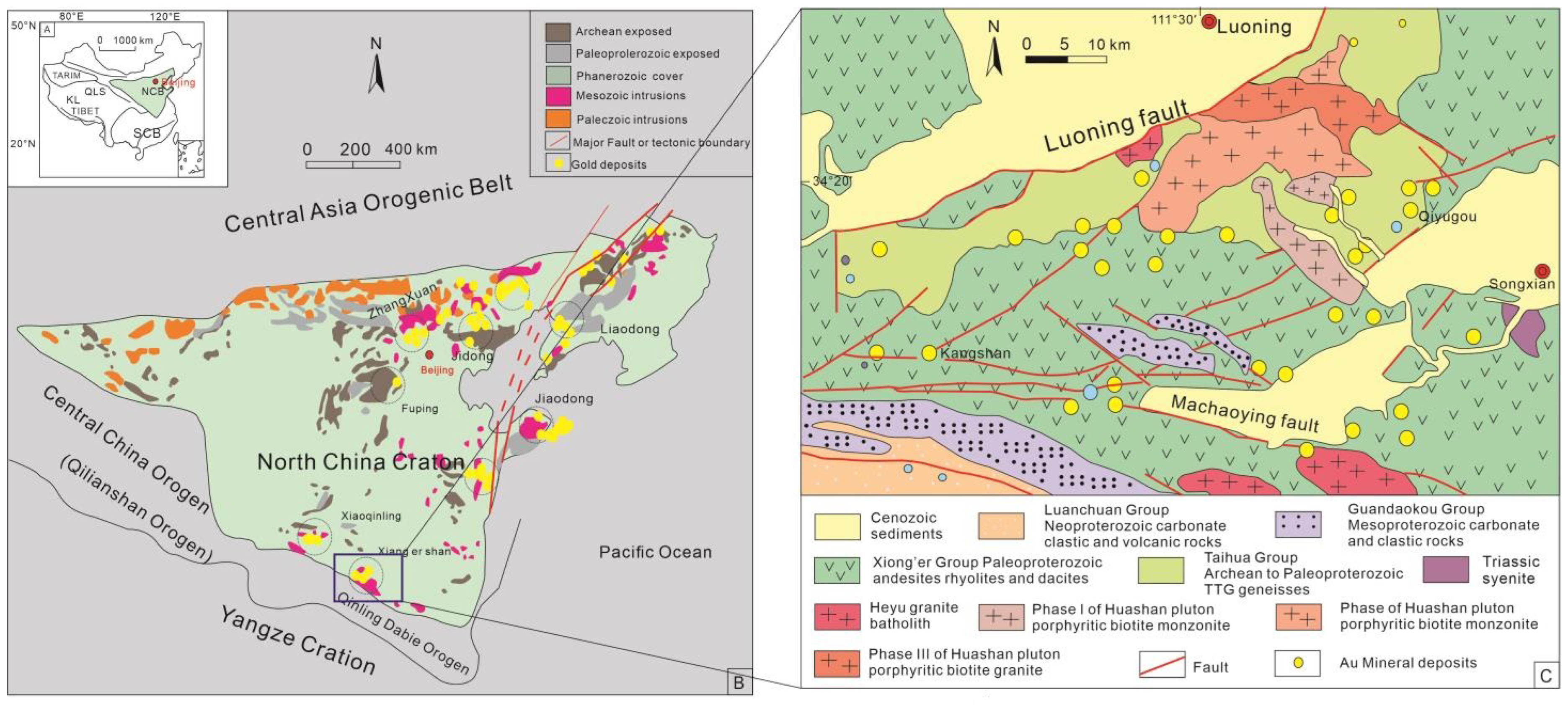
Figure 1. Simplified geological maps of the Xiong’ershan, Henan province in China: (A) map showing the location of the NCC; (B) the location of the Xiong’ershan ore clusters within the CNN (modified after [123,124,125]); and (C) regional geologic map of Xiong’erhsan district and distribution of gold deposits in the region (modified after [126,127,128]).
Minerals 12 01621 g001
Figure 3. Distribution Histogram for Geological exploration dataset in the Xiong’ershan area.
Minerals 12 01621 g003
Figure 4. Evidence layers with major gold deposits: (ak) clr-transformed Au, Ag, Pb, Zn, Mo, W, Hg, Sb, As, PC1, PC2; and (lp) with gold deposits RGA, FB, FT, FID, GRB.
Minerals 12 01621 g004
Figure 5. Loading chart for the first and second principal components in the Xiong’er shan area.
Minerals 12 01621 g005
Figure 6. The kernel density map of parameter optimization based on random search and TPE on the test sets (iteration = 100).(ai) the parameter of n_estimators, learning rate, max_depth, max_feature, subsample, min_impurity, train_time, loss, min_impurity_decrease.
Minerals 12 01621 g006
Figure 7. 3D visualization of the random search-GBDT model and TPE-GBDT model results: (a) random search-GBDT based on boosting hyperparameters; (b) TPE-GBDT based on boosting hyperparameters; (c) random search-GBDT based on weak learner hyperparameters; (d) and TPE-GBDT based on weak learner hyperparameters.
Minerals 12 01621 g007
Figure 8. The Accuracy of five-fold cross-validation based on the GBDT model.
Minerals 12 01621 g008
Figure 9. The confusion matrix of the: (a) random search-GBDT; (b) TPE-GBDT model with the MS datasets; (c) random search-GBDT; and (d) TPE-GBDT model with the OS datasets.
Minerals 12 01621 g009
Figure 10. ROC curves of Random search-GBDT model and TPE-GBDT model.
Minerals 12 01621 g010
Figure 11. Predictive models of mineral prospectivity derived by: (a) random search-GBDT; and (b) TPE-GBDT models.
Minerals 12 01621 g011
Figure 12. Performance of the Random search-GBDT and TPE-GBDT models of mineral prospectivity measured by success rate curve.
Minerals 12 01621 g012
Figure 13. Predictive maps of: (a) random search-GBDT; and (b) TPE-GBDT models, showing favorable and non-favorable areas by a threshold value of the Max Youden index.
Minerals 12 01621 g013
Table 1. Categories of GBDT hyperparameters.
TypeParameter
boostingn_estimators, learning_rate, loss, alpha, init
Weak evaluator structurecriterion, max_depth, min_samples_split, min_samples_leaf,
min_weight_fraction_leaf, max_leaf_nodes, min_impurity_decrease
early stopvalidation_fraction, n_iter_no_change, tol, n_estimators_
Weak evaluator training datasubsample, max_features, random_state
othersccp_alpha, warm_start
Table 2. GBDT hyperparameters selected and default values in Sklearn.
ParameterFunction of ParametersDefault Value
lossloss function“deviance”
criterionImpurity measurement index of weak estimate when branching“friedman_mse”
n_estimatorsThe Actual number of iterations100
learning_rateWeighted summation process affecting weak estimator results0.1
max_featuresMaximum number of features considered in constructing optimal CART tree modelNone
subsampleThe Proportion of random samples released from the full dataset before each CART tree is built1.0
max_depthMaximum allowable depth of weak estimator3
min_impurity_decreaseThe minimum reduction in impurity is allowed when the weak evaluator branches0.0
Table 3. GBDT parameter space for training datasets.
ParameterInitial Parameter SpaceFinal Parameter Space
loss[“deviance”,”exponential”][“deviance”,”exponential”]
criterion[“friedman_mse”, “squared_error”][“friedman_mse”, “squared_error”]
n_estimators (25,200,25) (55,200,1)
learning_rate (0.1,2.1,0.1) (0.05,1,0.005)
max_features (4,20,2) (1,16,1)
subsample (0.1,0.8,0.1) (0.5,1.0,0.05)
max_depth (2,30,2) (10,35,1)
min_impurity_decrease (0,5,1) (0,5,0.1)
Table 4. The Optimized parameters for the GBDT model.
ParameterParameter Value Based on the Random SearchParameter Value Based on the TPE
loss“deviance”“deviance”
criterion“friedman_mse”“friedman_mse”
n_estimators18669
learning_rate0.090.7
max_features912
subsample0.950.8
max_depth1210
min_impurity_decrease0.10.1
Table 5. The result of five-fold cross-validation for GBDT model.
ModelTrain AccuracyTest AccuracyFive-Fold Cross-Validation TimeDatasets
GBDT0.9810.9400.55 sMS
GBDT-Random1.0000.9633.16 s
GBDT-TPE1.0000.9660.71 s
GBDT1.0000.7540.07 sOS
GBDT-Random1.0000.7640.33 s
GBDT-TPE1.0000.7860.09 s
Table 6. The secondary indicators of the GBDT model base on the confusion matrix.
ModelAccuracyRecallPrecisionSpecificityDatasets
GBDT-Random0.95660.97910.9400.9322MS
GBDT-TPE0.95930.98440.9410.9322
GBDT-Random0.7770.6360.8750.857OS
GBDT-TPE0.8330.7270.8750.875
Publisher’s Note: MDPI stays neutral with regard to jurisdictional claims in published maps and institutional affiliations.