First High-Power CSEM Field Test in Saudi Arabia

Abstract

We conducted an initial high-power CSEM (controlled-source electromagnetic method) survey in a coastal salt-flat area in the broader area of Half Moon Bay, in the southern part of Dammam Peninsula in the eastern province of Saudi Arabia. The primary purpose of this work was to verify the technology, but we were also able to detect and characterize potential economic brines in the study area. For a high-quality data acquisition, several transmitter–receiver configurations, different acquisition parameters, and passive and active EM data were collected, evaluated, processed, and interpreted to characterize the subsurface. The long-offset EM (LOTEM) and the focused-source EM (FSEM) were the optimum configurations due to the high-quality of the collected data. This is a starting point for using the CSEM method towards the O&G, geothermal, CO₂ sequestration, groundwater, lithium brine, and other natural resources’ exploration and exploitation in the Gulf countries.

1. Introduction

Conventional and unconventional natural resource geophysics includes the use of proper methods for the exploration, characterization, and monitoring of conventional oilfields; shale hydrocarbon, geothermal energy, mineral, and groundwater exploration; CO₂ sequestration; and lithium brine extraction. In the oil and gas industry, active methods are often preferred over passive methods; the advantages lie in the complete control over the strength and waveform of the source signal and the possibility to tailor the source signal based on an area’s noise level. For all natural resources, passive and active electromagnetics have made significant technical and scientific contributions. However, characterizing the subsurface using surface geophysical methods has always been challenging. This is because the most common geophysical exploration method is seismic (particularly reflection), which is based on acoustic velocities that are very high in carbonates (the majority of the host rock in Saudi Arabia). Thus, this yields little information as low energy becomes diffusively backscattered.

On the other hand, electromagnetic (EM) methods have been widely used in geothermal, mineral, and oil and gas exploration due to their sensitivity to the subsurface bulk resistivity, which aids geological interpretation as the resistivity is correlated with a different rock matrix, porosities, and pore fluids filling the pore space. Moreover, the electromagnetic methods (EM) [1] in a tensor mode allow for the imaging of the fluids and the fracture zones in the carbonates [2,3,4,5,6,7,8]. Especially in the active (controlled-source EM-CSEM) EM methods, the source signal can be transmitted in multiple directions, and with several receivers, additional information regarding the electrical anisotropy of the underlying sediments can be acquired. Such is the case of shale formations that exhibit an inherently strong anisotropy. Furthermore, the combination of n boreholes with surface tensor EM measurements can be used to support a better correlation with seismic images [9,10]. In siliciclastic environments, the high resistivity contrast from replacing the reservoir fluid during the enhanced oil recovery (EOR) process from hydrocarbons to brines results in a strong EM anomalous response that can be easily interpreted for up to 3–5 km in depth, with a better resolution attainable using CSEM measurements rather than magnetotellurics (MT). Thus, the reason to apply CSEM instead of MT (passive) measurements is that the signal from the transmitter is much stronger than the Earth’s magnetic field and the background noise, and we can predict the signal using mathematical modeling [4,11]. Thus, CSEM often has higher resolution models than the passive MT surveys.

Furthermore, combining EM with microseismic and gravity information [12] often provides excellent results to overcome the inherent ambiguity of geophysical methods. Since fluids in carbonates are mostly in fractures with a lower density, combining resistivities from EM with densities from gravity measurements can enable an additional degree of targeting porosity and fluid variations in the reservoir rock [9]. The most significant potential for EM methods lies in monitoring any reservoir, as the response from the fluid movement will cause considerable signal changes above the noise level, accessed via a feasibility study before data acquisition.

Thus, the main purpose of using non-seismic methods (electromagnetic tensor measurements in combination with microseismic and gravity data) is to characterize and monitor the subsurface and to directly map the fluids and fracture direction [13,14,15,16]. While the measurements are—in principle—complementary, they also have an overlapping response. Where the different applied methods/measurements show similar anomalies, the fractures and their fluid content can be pinpointed. Moreover, the reservoir permeability can be estimated using tensor measurements and anisotropic models. Moreover, the target components, such as hydrocarbons (in oilfields) [17,18,19], hot water (in geothermal areas) [20,21], freshwater (in groundwater) [22,23,24,25], CCS (CO₂ capturing and storage) [16,26,27], minerals (in mining exploration) [28], and brine (in lithium exploration) [29,30] present a good to excellent (regarding conductivity and density) contrast.

Specifically, in geothermal exploration, EM passive methods such as MT and Audio Magnetotellurics (AMT) have been the industry standard due to the existing 3D interpretation tools [31]. Calibration against drilling results has been performed in several geothermal fields, and the correlation between resistivity, lithology, and temperature associated with the degree of hydrothermal alteration to the host materials has been well established. The higher temperatures and salinity of the pore fluids and increased rock alteration associated with geothermal areas often decrease the bulk resistivity in a rock mass, ideal for detection using MT/AMT. The bulk resistivity is further lowered if faults and fracture zones cross-cut the geothermal play [32,33].

Traditional exploration with EM methods requires these considerations to determine if the measured response matches the expected EM response for a charge reservoir and, if so, to estimate its lateral distribution and volume. However, for monitoring applications such as CCS (CO₂ Capturing and Storage), where time-lapse measurements are acquired, CSEM surveys are designed to measure the minor but detectable variations in the signal from the injected CO₂. Thus, the primary concern must be collecting the highest-quality data and maintaining data integrity through processing. This includes optimization during planning and feasibility, careful and consistent quality checks in the field, and transparent and repeatable post-processing steps [34].

In recent years, lithium exploration has been of great interest as lithium is one of the leading materials for manufacturing batteries [35]. Although recent evaluations of Transient EM (TEM) and controlled-source AMT (CSAMT) [36,37] have concluded that these methods do not provide the necessary depth of investigation, the highly conductive nature of lithium brine requires low-frequency bands to reach the depths of interest; thus, MT is probably the most robust technique for the exploration of the lithium problem.

Here, the first high-power CSEM survey has been conducted by the King Fahd University of Petroleum and Minerals (KFUPM) in the broader area of Half Moon Bay, which lies in the southern part of the Dammam Peninsula in the eastern province of Saudi Arabia. The main purpose of the EM geophysical survey was the deep subsurface characterization of the coastal saline salt flats and the detection of the brines in the study area.

To ensure the efficiency of the applied techniques and the acquisition of high-quality data, several transmitter–receiver configurations, different acquisition parameters, and passive and active EM data were collected, evaluated, processed, and interpreted to characterize the subsurface. In Saudi Arabia, this survey is the starting point for using the CSEM method in the exploration and exploitation of O&G, geothermal, CO₂ sequestration, groundwater, lithium brine, and other natural resources.

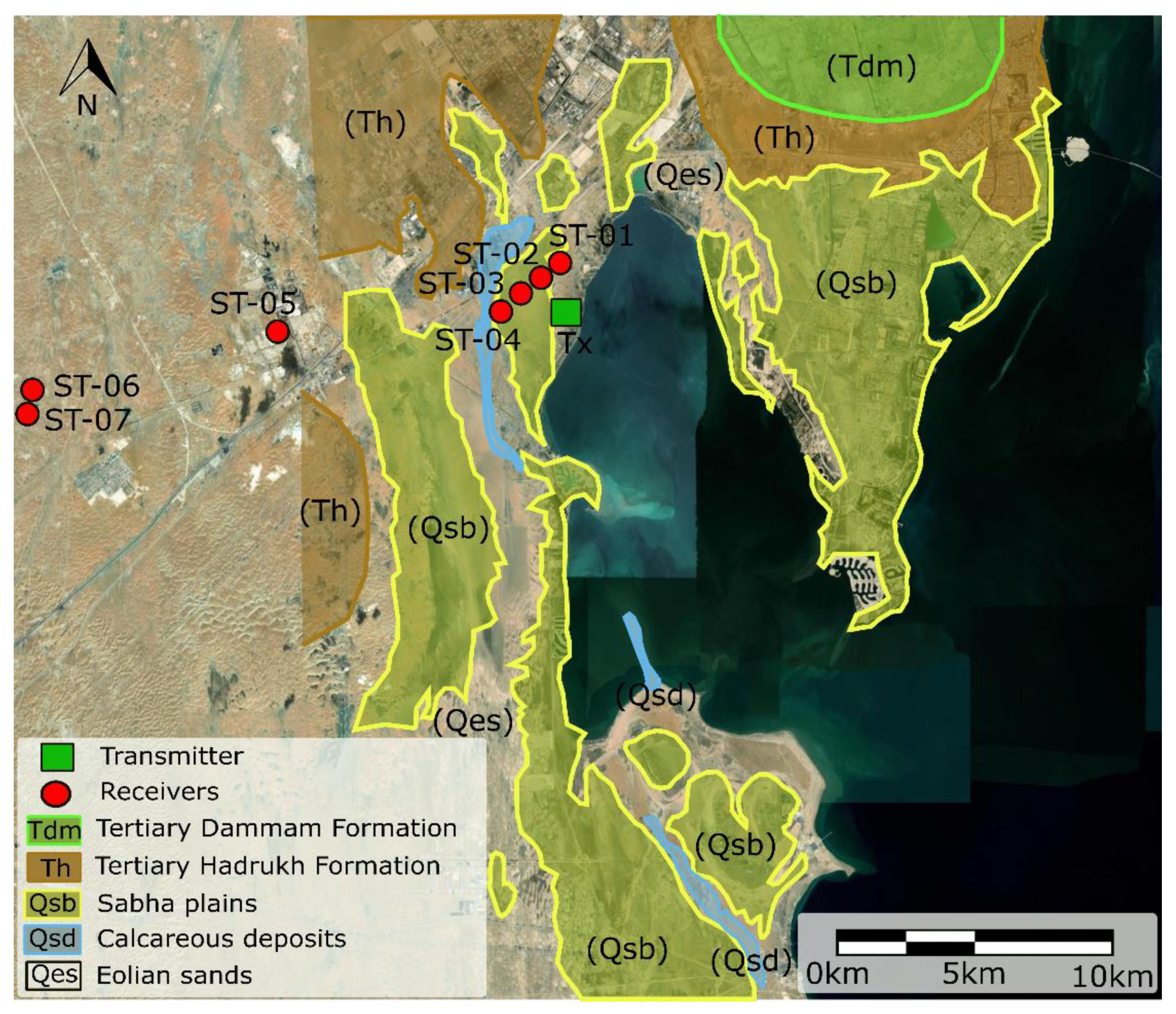
2. Geological Setting of the Study Area

The Half Moon Bay study area is known as Dawhat Zulumor Khaleej Nisf Al-Qamar and is in the southern part of the Dammam Peninsula. The coastal area consists of sand, sabkhas, and dunes with a maximum thickness of 50 m (Figure 1). The specific area has a fascinating geology since mixing marine and continental siliciclastic within a sabkha environment can be observed at several scales. The deeper formations have a Tertiary age and have been deformed and uplifted during the development of the Dammam (salt) Dome [38,39,40]. The moderate uplift has caused progressive sea regression and the formation of vast coastal sabkhas, partially covered by the dunes. The Late Tertiary Hadrukh Formation overlies the Tertiary Dammam Formation (Tdm) (Th). The quaternary deposits that cover the greater bay region consist of silt deposits on sabkha plains (Qsb), eolian sands (Qes), and calcareous deposits on the Flandrian high shore (Qcd) (Figure 1). A sabkha is often covered by mud comprising calcite, aragonite, gypsum, anhydrite, and halite combined with varying proportions of (mostly eolian) quartz sand. Weijermars [39] reported finding alternate layers of horizontally folded eolian sand sheets, cross-bedded eolian dune deposits, marine beach rock, and coquina beneath the sabkha layer. However, there is no evidence (from boreholes and logs in the study area) of the stratigraphy with information about the thicknesses of the different formations. Seber et al. [41] constructed a database (covering the study area) based on available geological, geophysical (gravity, seismological and seismic), and remote-sensing data (different satellite images), and they were able, with limited resolution, to provide the depth to the metamorphic basement, which in our study area was found at a depth of 5–6 km. Therefore, the geological information from Weijermars [39] and the preliminary depth to the bedrock model from Seber et al. [41] can be used to build the conceptual/initial model of the study area.

3. Methodology

Herein, we describe the CSEM methodology and data processing methods used in this survey. For the MT method, we refer to the already-cited references [1,10,18].

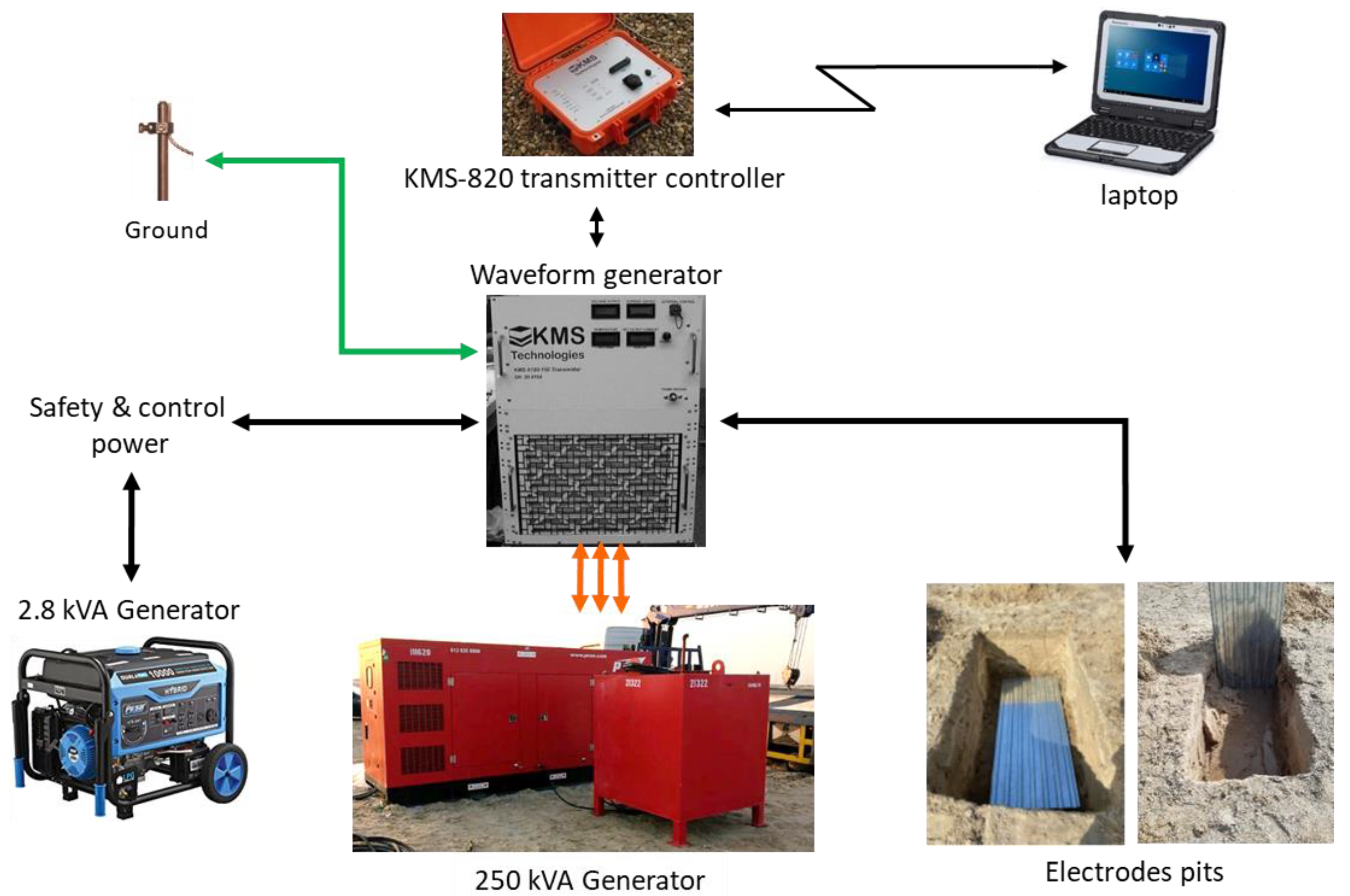
3.1. Data Acquisition

A five-day field campaign was conducted from 28 December 2021 to 2 January 2022 in the broader Half Moon area in East Province in Saudi Arabia. A high-power CSEM transmitter and seven receivers were installed for active and passive EM measurements. The transmitter was set up about 1 km west of the shoreline, and the measurements were conducted at different distances (930 m to 20 km) from the transmitter to the southwest, as shown in Figure 1. The transmitter dipole electrodes were installed within the sabkha, a formation rich in evaporite-saline minerals typically accumulating below the surface of mudflats or sandflats. Figure 2 describes the layout of the transmitter’s components. A 250 kVA three-phase generator was connected to a KMS-5100 transmitter switch box for the current injection via the electrodes. A KMS-820-transmitter controller unit and a laptop were connected to the transmitter sending the data in real-time to the Cloud. It should be mentioned that the new KFUPM’s complete field array EM system is cloud-based, and the interpreter can apply the quality control and assurance in real-time, requesting changes in the acquisition parameters or even the used geometries [42]. The generator’s power is isolated from the transmitter switch box so that it can be turned on/off if the power generator fails, thus avoiding ground loops and maintaining overall safety.

The transmitter dipole has two sides/electrodes (east and west) and are separated by 1 km in length (Figure 3A). There are six (6) pits of roughly 1 m depth for each electrode side, consisting of a 1 m × 2 m corrugated metal sheets 3 m apart. For the current injection, typical time-domain waveforms were applied, namely, (1) Bipolar reversing 100% duty cycle and (2) Bipolar 50% duty cycle, but any other waveforms that can be selected via the transmitter controller were used. The transmitter current is injected constantly for a 100% duty cycle; only the polarity switches periodically. For the 50% duty cycle, the transmitter periodically switches on–off positive and on–off negative. The off time is used for obtaining a reference level, whereas in the 100% duty cycle waveform, the reference level is derived from the transient leader (data before switching). Several tests were performed for both waveform types before the measurement to verify the current output stability. During the tests, the injected current varied from 40–200 Amps, and the voltage was between 51–220 Volts. The duration of the injection current also ranged from 5 min to a maximum of 30 min.

Table 1. The locations of the MT/CSEM receivers’ coordinates are presented.

Station	Coordinates	Elevation (m)	Distance from Tx (m)
ST-01	26°09.4489′ N 49°59.4567′ E	0	931
ST-02	26°09.4057′ N 49°59.3446′ E	0	1005
ST-03	26°09.3652′ N 49°59.2511′ E	0	1092
ST-04	26°09.2756′ N 49°59.0329′ E	0	1357
ST-05	26°08.6684′ N 49°53.4044′ E	3	10,700
ST-06	26°07.0260′ N 49°47.6663′ E	44	20,584
ST-07	26°06.8866′ N 49°47.5993′ E	44	20,736

lists the receiver coordinates and their distances from the transmitter for both the near Tx sites (ST-01 to ST-04) and the far from Tx sites (ST-05 to ST-07). The locations were selected to test the transmitter and the signal behavior at different distances. Figure 3B shows the receivers’ setup at each site. For MT, we used four electric field electrodes (Ex₁, Ex₂, Ey₁, and Ey₂) and three magnetic coils (Hx, Hy, and Hz). For the CSEM survey, two different layouts were applied. The LOTEM (long offset transient electromagnetic method) uses the standard CSEM layout, and the Focused-Source Electromagnetic (FSEM-4 electric fields) with the airloop, an S20 coil, which measures the vertical time-derivative of the magnetic field and a fifth electrode in the center of the array. The FSEM method was introduced by Davydycheva et al. [43] and was first followed by Davydycheva and Rykhlinski [13]. The goal of the FSEM method is to obtain deep resistivity data by focusing the EM field vertically and eliminating the horizontal component of electric current density. FSEM improves the conventional CSEM method, which has significantly higher spatial resolution and provides deeper resistivity data [16].

Before applying any task or starting any measurements at the installed stations, the ground resistance—using a digital multimeter for both Ex (north–south electrical field) and Ey (east–west electrical field)—on each receiver station is measured to ensure good (1–3 kohm) contact resistance between electrodes. When the measured resistance was greater than 3 kohm, bentonite (or other clay materials/powders) was added at the bottom of the non-polarized electrodes, and more saline water was added to achieve an acceptable contact resistance.

The CSEM (active) measurements were recorded during the day with a 1 kHz sampling frequency, which was switched to MT (passive) during the night with a 40 Hz sampling rate. However, we also utilized MT data from the 1 kHz sampling rate before and after the transmitter was switched on. The detailed description of the type of recording per day is listed in

Table 2. Types of EM measurements applied by site and for each day.

Station	Day 1 (Tx Test and MT)	Day 2 (CSEM and MT)	Day 3 (CSEM and MT)	Day 4 (CSEM and MT)
ST-01	STD MT	LOTEM	STD MT, LOTEM, S20	STD MT, S20
ST-02	STD MT	STD MT, S20	STD MT, S20	STD MT, S20
ST-03	FSEM, STD MT	STD MT, S20	STD MT, S20	STD MT, S20
ST-04	FSEM, STD MT	LOTEM	STD MT, LOTEM, S20	STD MT, S20
ST-05	-	-	-	LOTEM
ST-06	-	-	-	LOTEM
ST-07	-	-	-	STD MT, LOTEM

STD MT—Standard MT, LOTEM—long offset transient EM, S20—airloop, and FSEM—focused-source EM.

. We were able to record CSEM data from day 2 to day 4 with trial testing conducted on day 1. During the CSEM measurements, we tested both 50% and 100% duty cycles from the transmitter waveform with a 6 s switching time. Immediately after the first recording, all receivers were checked to see whether they were saturated or not, ensuring that the recorded signal was correctly within the instrument’s measurement range. Figure 4 shows a raw time-series example displayed with the KMS-820 acquisition program for both active (CSEM) and passive (MT) EM measurements. Both measuring modes (MT and CSEM) showed a clear recorded signal for all the E-field and H-field-installed components. The acquisition system stores the transmitter operation logs during the CSEM data acquisition, allowing the analyst to correlate any potential issues in the receivers’ records against any problems that might have occurred during the transmission.

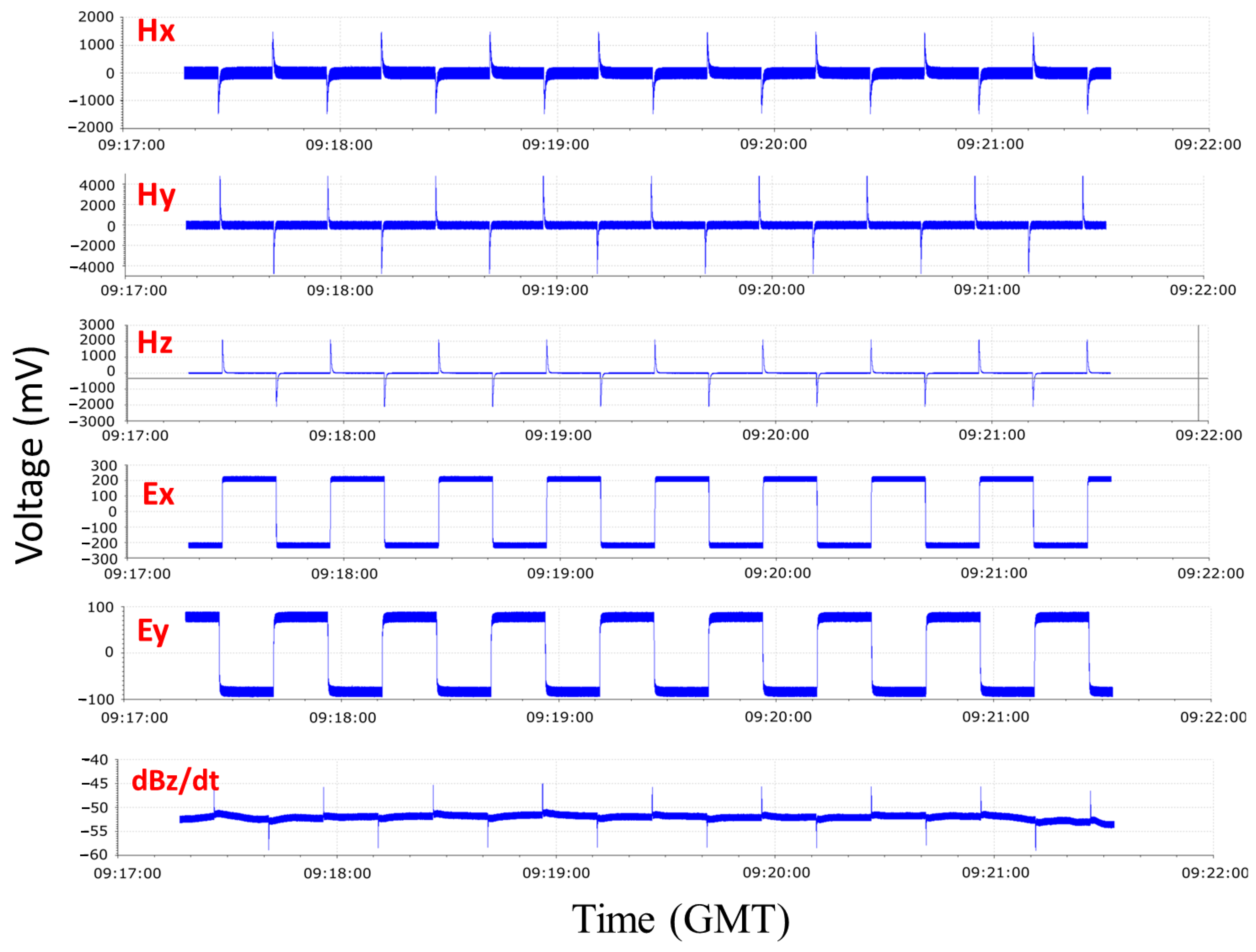
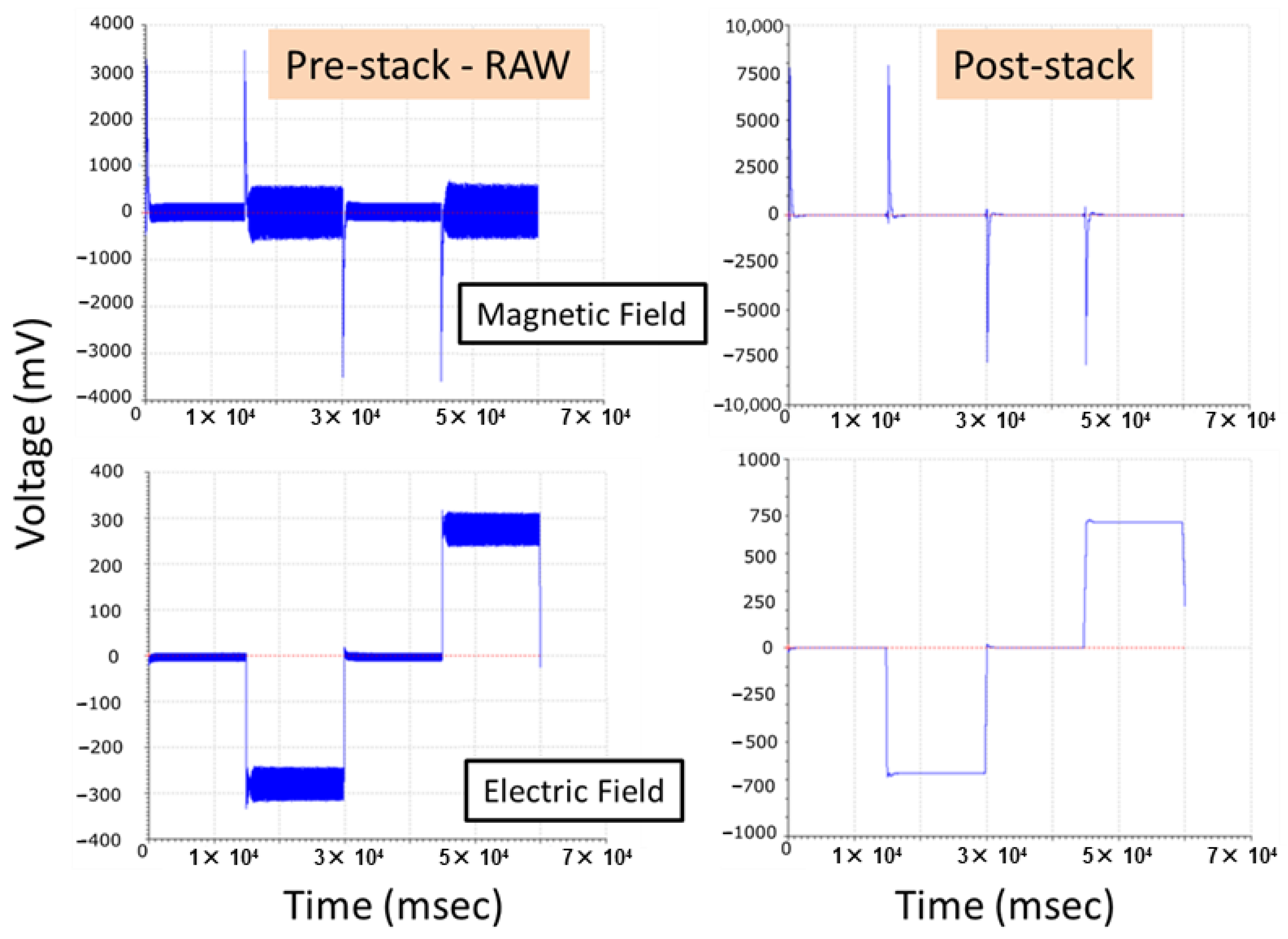
3.2. Data Processing

During data acquisition, the output (recorded) signal, as the Earth’s response, is produced by the combination of an input (magnetic field for MT and injected current for CSEM surveys) signal with the effect of the data generation process and Earth’s response [43]. As in all geophysical methods and forms of data acquisition, most of an EM measurement’s signal is “contaminated” by periodic and sporadic noise, which directly affects the signal-to-noise ratio (SNR). High-voltage power lines close to the study area usually produce periodic noise. Sporadic noise can be seen in time series as spikes, steeps, or drifts and is caused by other types of noise sources, such as fences, switching power supplies, machinery, etc. Those noises must be eliminated or reduced through data filtering and processing to increase the SNR and obtain the “true” signal from the acquired data. Since we have two different EM measurements, namely, CSEM as an active method and MT as a passive method, they need to be separated and processed independently before interpreting the data to produce a unique model for the subsurface.

The CSEM data, including LOTEM, must be processed using special software to perform data quality assurance, data merge/separation, and data quality control, including filtering. The main objective of this stage is to minimize the influence of the processing on the acquired signal, removing the recorded noise and improving the quality of the collected data. The data’s quality assurance incorporates time-series visualization, the files’ header check, the instrument’s calibration verification, and the configuration’s editing. All information available in the raw data, such as recording time, sensor types, channel positioning, sampling frequency, file name, etc., need to be checked using the KMSProQA program to ensure that it is all correct. Figure 5 and Figure 6 visualize the raw data using KMSProQA for CSEM 50% duty cycle data and CSEM 100% duty cycle, respectively. The recording time, the sensor types, and other parameters can be visibly clarified. At this stage, the harmonic noise can also be detected by calculating the spectrum using KMSProQA as shown in Figure 7. We clearly recognize several noises at 23 Hz and 60 Hz shown as spikes in the spectrum. We suggest that both are harmonic noises from the generator and the power line.

Since the receivers’ records contain both active and passive EM measurements with different frequency rates, these must be separated by cropping and merging before the quality control processing. During a data merge, the receiver and transmitter’s time-series synchronization, a time shift correction, the component’s polarity flip, and a re-sampling frequency, if required, should be applied. Once the merge has been completed, all recorded time series for both electric and magnetic components at each receiver and transmitter are available for further processing. The next step is the data quality control process using the KMSProQC software, which is a crucial stage where noise is to be removed from the data via pre-stacking, stacking, and post-stacking processes. During pre-stacking, data are filtered to remove the noise, such as that recognized from the spectrum. Different filters were tested, including the time and frequency domain notch filter, lock-in filter, and low-pass filter, as well as the thresholding frequency as an additional parameter.

The notch filter removes a narrow frequency band and keeps the remaining spectrum unchanged [44]. In our case, standard recursive filters have been modified for LOTEM to avoid signal amplitude attenuation [45]. However, a different filter, such as a lock-in filter, is required, because in some cases, the transient cannot be recovered from the signal by applying the notch filter. Specifically, the lock-in filter adapts to the phase changes of the periodic noise and subtracts the results from the acquired data [45]. In contrast to periodic noise, sporadic noise from natural sources is difficult to recognize and, consequently, cannot be removed by filters. This kind of noise can be removed using mainly stacking techniques (Figure 8). Among the stacking methods often tested are mean, median, RME (regression M-estimate) Hampel, trimmed mean, and selective stacking, with selective stacking being the preferred method. The last step applied in the data’s quality control process is the post-stack time variant smoothing to ensure that the processed data is as smooth as possible. After applying all these data-processing techniques, a smoothed transient, as shown in Figure 9, is acquired.

In the same way as CSEM, the MT data must be processed before any interpretation. To process MT data, the KMSProMT software should be used for filtering, stacking, and estimating the impedance tensor, and the KMSProTF program to deal with transfer function results. As already stated, most of the MT data were measured with a sampling rate of 40 Hz; however, some of the data were recorded with a 1 kHz sampling rate. Therefore, before applying any filters, MT data were separated from CSEM. During filtering, low frequency (LF) filter parameters (short FFT window of 64 samples) were chosen to deal with the 40 Hz sampling rate data, and high frequency (HF) parameters (FFT window of 65,000 samples) to filter 1 kHz sampling rate data. For this study, and from the MT transfer functions (phase tensor and tipper vector), only the phase tensor was calculated. The output of the MT data processing was calculated with robust statistics and exported in EDI (Electrical Data Interchange) format containing the apparent resistivity (ρ_a), phase (φ), and impedance tensor (Z). Figure 10 and Figure 11 show an example of raw and processed MT data, respectively.

Generally speaking, the aforementioned processing steps produced the impedance, tipper, and spectral density matrix in EDI files following the standard SEG format. The EDI files can be imported to several commercial or academic software programs for further processing, such as Interpex IX1D, WinGlink, Geotools, ZondMT2D, EMUPLUS, ModEM3D, and others.

One dimensional (1D) analyses for each sounding for both MT and CSEM (LOTEM) data were performed. Based on the average resistivity of the study area of 0.7 Ohm.m and the frequency of the injected current (max of 100 s), a skin depth of 4.1 km was estimated and used for all of our 1D inversions [46]. The 1D inversion for MT data was performed using Interpex IX1D software for XY, YX, and the invariant of both datasets using OCCAM’s inversion technique. The different number of layers and various models such as Bostick and Niblett were also tested during the 1D analysis process. To apply an uncertainty analysis, the model equivalence was used by indicating the range (thicknesses and resistivities) of models that could fit the acquired data. The 1D inversion results for MT data can be seen in Figure 12, with RMS varying between 1.2 to 4.9.

For the LOTEM-CSEM data, the 1D inversion was performed using EMUPLUS software, which serves as the standard 1D inversion tool for interpreting any processed transients. In our case, both electric and magnetic field data were inverted. Some preliminary processes must be performed before inversion, such as data normalization, conversion into apparent resistivities (early and late), and ensuring the correctness of the required information, such as offset, current, coordinate, etc. The starting model used was a homogeneous half-space to yield the 1D model of OCCAM’s inversion. The result from the OCCAM’s inversion is further analyzed using cumulative conductance and transverse resistance to generate the starting model for the subsequent Marquardt inversion (layered model). Finally, we compare the inversion results from both LOTEM and MT data. Figure 13 and Figure 14 show the inversion data fits and comparisons with MT results for electric and magnetic field data, respectively, in ST-03. Both figures indicate good agreement between the predicted model from LOTEM and the MT result.

For the inversion of the far-field soundings, namely, ST-05 at almost 10 km from Tx and ST-06 and ST-07 at a distance of about 20 km from the Tx (transmitter), the same inversion methods and regularization parameters as above were used, but several tests were applied prior the final selected model. Specifically, to ensure the robustness of the final inverted model for ST-07 CSEM sounding, the models that resulted from using the complete setup of E- and H-field were compared with the model that resulted from replacing the noisy Hz component with the calibrated airloop. Moreover, the same initial resistivity model extracted from the ST-07 MT sounding was used for all the tests. The number of layers was also varied, specifically, from 5–8 layers, and in some of the tests, the early or the early/late times were masked before the final inversion. Overall, the fitting of the final inverted model was acceptable, with an average misfit of 8.97.

After the individual inversion of all the acquired MT/CSEM soundings, the four near the Tx (ST-01–ST-04), the soundings collected along an SW–NE profile, were reprocessed by applying a 2D inversion. For the 2-D inversion of the near field EM soundings, the REBOCC code [47], with the modification from Pedersen and Engels [48] to allow for the inversion of the determinant of the impedance tensor, was used [21]. The average determinant of the impedance tensor, Zdet, is given by, Zdet = (ZxxZyy − ZxyZyx)1/2, where Zxx, Zxy, Zyx, and Zyy are the impedance tensor elements [49]. When inverting determinant data, the strike determination is less critical than inverting E- and H-polarization data [50]. The possible static shift correction is also more convenient in the case of the rotationally invariant determinant data, as no decomposition to the E- and the H-polarization modes is necessary before the correction. Further information on the 2-D inversion of determinant MT data can be found in Pedersen and Engels [48] and Smirnov and Pedersen [50]. The data fits for the inversion models are good, generally within the 1.5% root-mean-square deviation (RMS) value.

4. Results

The 1D inversion results for the first four soundings, those nearest to the transmitter (Tx), are presented in Figure 12. All the data were inverted, assuming an initial 5-layer model, and the final inverted model showed a similar behavior. A very low resistivity layer, below 1 Ohm.m, was detected in all four soundings below the depth of 300–350 m. The bedrock, identified as the more resistive formation, was detected at a depth of 2 km below the ground’s surface. The equivalent models for all four final inverted models are shown with green dashed lines. It should be noted that the variability of the equivalent models is limited.

The final 1D inversion model for the collected CSEM data in ST-03 is presented in Figure 13. The calculated final inverted model agrees with the field data, as shown in Figure 13, the left diagram. A discrepancy was only found in the late times, after 2.5 s. For the inversion of the CSEM data, the final inverted resistivity model from the processing of the MT data at the same station was used as an initial model (Figure 13, right model with the black line). The final inverted model for ST-03 from the processing of the CSEM data is not differentiated from the initial model (form MT data) used. A very low resistivity layer, with a resistivity of about 0.3 Ohm.m, was detected at a depth of 300–350 m below the ground surface with a thickness of almost 1 km.

The final 1D inversion model for the collected CSEM data in ST-07, around 20 km away from the transmitter (Tx), is presented in Figure 14. For the inversion of the CSEM data, the final inverted resistivity model from the processing of the MT data at the same station was used as an initial model (Figure 14, the model with the turquoise line). An initial model of 4-layers was also used for this inversion and interpretation since we did not expect, based on the geology of the study area, more layers or more than four units with different geophysical signatures. During the processing, and to ensure the reliability and robustness of the final inverted model, a different number of layers and data (masking the early time and/or very late (noisy) times) used for the inversion model were tested and evaluated. The final inverted model for ST-07, 20 km away from Tx, is presented in Figure 14 (model on the right). The calculated misfit is 8.97. Based on the resulting final resistivity model, after the depth of 1.3 km, the resistivity reached 3.1 Ohm.m and a very low resistivity layer, with a resistivity of about 0.1 Ohm.m, was detected at a depth of 3 km below the ground surface.

The final 2D inversion model using the REBOCC code for the SW–NE profile, composed of the ST-01 to ST-04, is shown in Figure 15. It is quite risky to apply 2D inversion on only four soundings, but we decided to do so to compare the final tomogra phic image with the final 1D inverted models, as presented in Figure 12. A very low resistivity anomaly with a resistivity of 0.3 Ohm.m was detected at a depth of 350 m below the ground surface. This finding is in agreement with the 1D models in Figure 12. This very conductive zone seems to extend below the maximum depth of the model, that is, 1 km.

5. Conclusions

As we enter the energy transition era, EM methods in general, and specifically CSEM surveying, are becoming more frequently used for reservoir-monitoring applications such as geothermal production, CO₂ injection monitoring, or Enhanced Oil Recovery (EOR), where fluid movements provide essential information. This is often executed by combining borehole and surface measurements with permanent or semi-permanent sensors and time-lapse acquisition.

The first CSEM survey using a high-power transmitter for the characterization of the flat salt coastal area of the Half Moon Bay in the Eastern Province of Saudi Arabia was completed successfully. Best practices were followed to setup and test the transmitter electrodes. Different receiver configurations were laid to acquire alternative LOTEM, FSEM, and MT data. All the data were obtained as planned, and processing workflows followed uneventfully. There were no HSE accidents or incidents during the acquisition. The CSEM data are of a high quality as this was monitored in real-time during the acquisition and later confirmed during the quality control process. As displayed in Figure 5, Figure 6, and Figure 8, the raw data clearly showed the shape of the transmitted waveform in the electric field components and the expected impulse response for the magnetic field components. The output transients, resulting from the processing workflow that was followed, yielded smooth transients adequate for further interpretation. The percentage of transients decaying evaluates the quality of a transient with respect to the reference level within the switching time interval and its smoothness. High-quality transients often decay >90% in amplitude within a time window. Ultimately, the quality of these transients determined the quality of the interpretation results. Likewise, MT data have good quality, where the apparent resistivity resulting from the processing of different sample rates can be further interpreted.

The high-resolution MT/CSEM survey in the study area discovered a thick, very low resistivity anomaly, with resistivities around 0.3 Ohm.m, much lower than the expected resistivity for brines (around 2 Ohm.m) [51]. Based on the international references and the characteristics of the depositional environment of the study area, such low (0.3 Ohm.m) resistivities can be associated with lithium deposits. However, further studies, such as exploratory boreholes and sampling, are needed to model the salar’s types, the brine’s chemistry and quality, and to verify these first assumptions about the study area [52,53,54]. Nevertheless, the current EM survey identified a potentially economic brine.

In summary, electromagnetic methods cover a range of applications, particularly those of interest during the energy transition and the development of mineral resources in Saudi Arabia, in accordance with the pillars of VISION 2030.

References

1. Vozoff, K. 8. The Magnetotelluric Method. In Electromagnetic Methods in Applied Geophysics; Society of Exploration Geophysicists: Houston, TX, USA, 1991; pp. 641–712. [Google Scholar]
2. Colombo, D.; McNeice, G.; Curiel, E.S.; Fox, A. Full tensor CSEM and MT for subsalt structural imaging in the Red Sea: Implications for seismic and electromagnetic integration. Lead. Edge 2013, 32, 436–449. [Google Scholar] [CrossRef]
3. Colombo, D.; Keho, T.; McNeice, G. Integrated seismic-electromagnetic workflow for sub-basalt exploration in northwest Saudi Arabia. Lead. Edge 2012, 31, 42–52. [Google Scholar] [CrossRef]
4. Colombo, D.; Dasgupta, S.; Strack, K.M.; Yu, G. Results of Feasibility Study of Surface-to-Borehole Time-Domain CSEM for Water-Oil Fluid Substitution in Ghawar Field, Saudi Arabia. In Proceedings of the GEO 2010, Manama, Bahrain, 7–10 March 2010. [Google Scholar]
5. Sheard, S.N.; Ritchie, T.J.; Christopherson, K.R.; Brand, E. Mining, Environmental, Petroleum, and Engineering Industry Applications of Electromagnetic Techniques in Geophysics. Surv. Geophys. 2005, 26, 653–669. [Google Scholar] [CrossRef]
6. Strack, K.M. Future Directions of Electromagnetic Methods for Hydrocarbon Applications. Surv. Geophys. 2014, 35, 157–177. [Google Scholar] [CrossRef]
7. Streich, R. Controlled-Source Electromagnetic Approaches for Hydrocarbon Exploration and Monitoring on Land. Surv. Geophys. 2016, 37, 47–80. [Google Scholar] [CrossRef]
8. Tietze, K.; Ritter, O.; Veeken, P. Controlled-source electromagnetic monitoring of reservoir oil saturation using a novel borehole-to-surface configuration. Geophys. Prospect. 2015, 63, 1468–1490. [Google Scholar] [CrossRef]
9. Henke, C.H.; Krieger, M.H.; Strack, K.; Zerilli, A. Subsalt imaging in northern Germany using multiphysics (magnetotellurics, gravity, and seismic). Interpretation 2020, 8, SQ15–SQ24. [Google Scholar] [CrossRef]
10. Strack, K.; Davydycheva, S.; Hanstein, T.; Smirnov, M. A new array system for multiphysics (MT, LOTEM, and microseismics) with focus on reservoir monitoring. AIP Conf. Proc. 2017, 1861, 020001. [Google Scholar]
11. Hu, W.; Yan, L.; Su, Z.; Zheng, R.; Strack, K. Array TEM sounding and application for reservoir monitoring. In Proceedings of the SEG Technical Program Expanded Abstracts 2008; Society of Exploration Geophysicists: Houston, TX, USA, 2008; pp. 634–638. [Google Scholar]
12. Demirci, İ.; Dikmen, Ü.; Candansayar, M.E. Two-dimensional joint inversion of Magnetotelluric and local earthquake data: Discussion on the contribution to the solution of deep subsurface structures. Phys. Earth Planet. Inter. 2018, 275, 56–68. [Google Scholar] [CrossRef]
13. Davydycheva, S.; Rykhlinski, N. Focused-source EM survey versus time-domain and frequency-domain CSEM. Lead. Edge 2009, 28, 944–949. [Google Scholar] [CrossRef]
14. Davydycheva, S.; Rykhlinski, N. Focused-source electromagnetic survey versus standard CSEM: 3D modeling in complex geometries. Geophysics 2011, 76, F27–F41. [Google Scholar] [CrossRef]
15. Demirci, İ.; Candansayar, M.E.; Vafidis, A.; Soupios, P. Two dimensional joint inversion of direct current resistivity, radio-magnetotelluric and seismic refraction data: An application from Bafra Plain, Turkey. J. Appl. Geophys. 2017, 139, 316–330. [Google Scholar] [CrossRef]
16. Strack, K.; Davydycheva, S. Using Electromagnetics to Map Lateral Fluid Variations in Carbonates in SE Asia. In New Approaches in Engineering Research; Book Publisher International (a part of SCIENCEDOMAIN International): Dulles, Virginia, 2021; Volume 2, pp. 69–79. [Google Scholar]
17. Palisch, T.; Al-Tailji, W.; Bartel, L.; Cannan, C.; Zhang, J.; Czapski, M.; Lynch, K. Far-Field Proppant Detection Using Electromagnetic Methods-Latest Field Results. In Proceedings of the SPE Hydraulic Fracturing Technology Conference and Exhibition, The Woodlands, Texas, USA, 24–26 January 2017. [Google Scholar]
18. Soupios, P.; Davydycheva, S.; Strack, K. Mapping fluid front in Carbonates using Electromagnetic. In Proceedings of the SPWLA Abu Dhabi Chapter Topical Conference, Reservoir Fluid Surveillance, Today and Beyond, Abu Dhabi, United Arab Emirates, 13–14 December 2021. [Google Scholar]
19. Strack, K.; Pandey, P. Exploration with controlled-source electromagnetics under basalt cover in India. Lead. Edge 2007, 26, 360–363. [Google Scholar] [CrossRef]
20. Aboud, E.; Wameyo, P.; Alqahtani, F.; Moufti, M.R. Imaging subsurface northern Rahat Volcanic Field, Madinah city, Saudi Arabia, using Magnetotelluric study. J. Appl. Geophys. 2018, 159, 564–572. [Google Scholar] [CrossRef]
21. Autio, U.; Smirnov, M.Y.; Savvaidis, A.; Soupios, P.; Bastani, M. Combining electromagnetic measurements in the Mygdonian sedimentary basin, Greece. J. Appl. Geophys. 2016, 135, 261–269. [Google Scholar] [CrossRef]
22. Demirci, İ.; Gündoğdu, N.Y.; Candansayar, M.E.; Soupios, P.; Vafidis, A.; Arslan, H. Determination and Evaluation of Saltwater Intrusion on Bafra Plain: Joint Interpretation of Geophysical, Hydrogeological and Hydrochemical Data. Pure Appl. Geophys. 2020, 177, 5621–5640. [Google Scholar] [CrossRef]
23. Haroon, A.; Lippert, K.; Mogilatov, V.; Tezkan, B. First application of the marine differential electric dipole for groundwater investigations: A case study from Bat Yam, Israel. Geophysics 2018, 83, B59–B76. [Google Scholar] [CrossRef]
24. Panagopoulos, G.; Soupios, P.; Vafidis, A.; Manoutsoglou, E. Integrated use of well and geophysical data for constructing 3D geological models in shallow aquifers: A case study at the Tymbakion basin, Crete, Greece. Environ. Earth Sci. 2021, 80, 142. [Google Scholar] [CrossRef]
25. Rani, P.; Soupios, P.; Barsukov, P. Regional tectonic model of Southern, Central part of the Mygdonian basin (Northern Greece) by applying 3D Transient Electromagnetic Modeling. J. Appl. Geophys. 2020, 176, 104008. [Google Scholar] [CrossRef]
26. He, Z.; Hu, Z.; Gao, Y.; He, L.; Meng, C.; Yang, L. Field test of monitoring gas reservoir development using time-lapse continuous electromagnetic profile method. Geophysics 2015, 80, WA127–WA134. [Google Scholar] [CrossRef]
27. Hördt, A.; Andrieux, P.; Neubauer, F.M.; Rüter, H.; Vozoff, K. A first attempt at monitoring underground gas storage by means of time-lapse multichannel transient electromagnetics. Geophys. Prospect. 2000, 48, 489–509. [Google Scholar] [CrossRef]
28. Kalscheuer, T.; Juhojuntti, N.; Vaittinen, K. Two-Dimensional Magnetotelluric Modelling of Ore Deposits: Improvements in Model Constraints by Inclusion of Borehole Measurements. Surv. Geophys. 2018, 39, 467–507. [Google Scholar] [CrossRef]
29. Cabello, J. Lithium brine production, reserves, resources and exploration in Chile: An updated review. Ore Geol. Rev. 2021, 128, 103883. [Google Scholar] [CrossRef]
30. Wang, D.; Dai, H.; Liu, S.; Wang, C.; Yu, Y.; Dai, J.; Liu, L.; Yang, Y.; Ma, S. Research and exploration progress on lithium deposits in China. China Geol. 2020, 3, 137–152. [Google Scholar] [CrossRef]
31. Martinez, Y.; Ashadi, A.; Hinojosa, H.; Soupios, P.; Strack, K. New High-Power Controlled Source Electromagnetic System for Geothermal Applications. In Proceedings of the Geothermal Rise Conference, Reno, NV, USA, 28–31 August 2022. [Google Scholar]
32. Tulinius, H.; Ádám, L.; Halldórsdóttir, H.; Yu, G.; Strack, K.; Allegar, N.; He, L.; He, Z. Exploring for geothermal reservoirs using broadband 2-D MT and gravity in Hungary. In Proceedings of the SEG Technical Program Expanded Abstracts 2008; Society of Exploration Geophysicists: Houston, TX, USA, 2008; pp. 1147–1151. [Google Scholar]
33. Tulinius, H.; Ádám, L.; Strack, K.M.; Yu, G.; He, L.F. Geothermal Exploration Using Integrated 2-D MT and Gravity Surveys in Hungary. In Proceedings of the 70th EAGE Conference and Exhibition Incorporating SPE EUROPEC 2008, Rome, Italy, 9–12 June 2008. [Google Scholar]
34. Barajas-Olalde, C.; Davydycheva, S.; Hanstein, T.; Laudal, D.; Martinez, Y.; MacLennan, K.; Mikula, S.; Adams, D.C.; Klapperich, R.J.; Peck, W.D. Using controlled-source electromagnetic (CSEM) for CO2 storage monitoring in the North Dakota CarbonSAFE project. In Proceedings of the First International Meeting for Applied Geoscience & Energy Expanded Abstracts, Houston, TX, USA, 26 September–1 October 2021; pp. 503–507. [Google Scholar]
35. Champion, D. Australian Resource Review: Lithium 2018; Geoscience Australia: Canberra, Australia, 2019; ISBN 978-1-925848-28-1. [Google Scholar]
36. Curcio, A.; Chanampa, E.; Cabanillas, L.; Piethe, R. An effective multiphysics toolkit for Lithium prospecting: From geophysics to the static reservoir model in Pozuelos salt flat, Argentina. In Proceedings of the The International Meeting for Applied Geoscience & Energy (IMAGE2022), Houston, TX, USA, 28 August–1 September 2022. [Google Scholar]
37. Curcio, A. President’s Page: Resources and geophysical opportunities in South America. Lead. Edge 2022, 41, 228–229. [Google Scholar] [CrossRef]
38. Tleel, J.W. Surface Geology of Dammam Dome, Eastern Province, Saudi Arabia. Am. Assoc. Pet. Geol. Bull. 1973, 57, A4304–A4316. [Google Scholar]
39. Weijermars, R. Quaternary Evolution of Dawhat Zulum (Half Moon Bay) Region Eastern Province, Saudi Arabia. GeoArabia 1999, 4, 71–90. [Google Scholar]
40. Weijermars, R. Surface Geology, Lithostratigraphy and Tertiary Growth of the Dammam Dome, Saudi Arabia: A New Field Guide. GeoArabia 1999, 4, 199–226. [Google Scholar] [CrossRef]
41. Seber, D.; Steer, D.; Sandvol, E.; Sandvol, C.; Brindisi, C.; Barazangi, M. Design and Development of Information Systems for the Geosciences: An Application to the Middle East. GeoArabia 2000, 5, 269–296. [Google Scholar] [CrossRef]
42. Strack, K.M.; Martinez, Y.L.; Passalacqua, H.; Xu, X. Cloud-Based Array Electromagnetics Contributing to Zero Carbon Footprint. In Proceedings of the Off-Shore Technology Conference; OTC: Houston, TX, USA, 2022. [Google Scholar]
43. Davydycheva, S.; Rykhlinski, N.; Legeido, P. Electrical-prospecting method for hydrocarbon search using the induced-polarization effect. Geophysics 2006, 71, G179–G189. [Google Scholar] [CrossRef]
44. Claerbout, J.F. Fundamentals of Geophysical Data Processing with Applications to Petroleum Prospecting; Blackwell Science Inc.: Osney Mead, Oxford, UK, 1985; ISBN 978-0865423053. [Google Scholar]
45. Strack, K. Exploration with Deep Transient Electromagnetics; Elsevier: Amsterdam, The Netherands, 1992; ISBN 978-0444895417. [Google Scholar]
46. Zhdanov, M.S. Magnetotelluric and Magnetovariational Methods. In Foundations of Geophysical Electromagnetic Theory and Methods; Elsevier: Amsterdam, The Netherands, 2018; pp. 495–584. [Google Scholar]
47. Siripunvaraporn, W.; Egbert, G. An efficient data-subspace inversion method for 2-D magnetotelluric data. Geophysics 2000, 65, 791–803. [Google Scholar] [CrossRef]
48. Pedersen, L.B.; Engels, M. Routine 2D inversion of magnetotelluric data using the determinant of the impedance tensor. Geophysics 2005, 70, G33–G41. [Google Scholar] [CrossRef]
49. Berdichevsky, M.; Dimitriev, V. Basic Principles of Interpretation of Magnetotelluric Sounding Curves. In Geolelectric and Geothermal Studies; Adam, A., Ed.; KAPG Geophysical Monograph, Akademiai Kaido: Budapest, Hungary, 1976; pp. 165–221. [Google Scholar]
50. Smirnov, M.Y.; Pedersen, L.B. Magnetotelluric measurements across the Sorgenfrei-Tornquist Zone in southern Sweden and Denmark. Geophys. J. Int. 2009, 176, 443–456. [Google Scholar] [CrossRef]
51. Falcon-Suarez, I.; Marín-Moreno, H.; Browning, F.; Lichtschlag, A.; Robert, K.; North, L.J.; Best, A.I. Experimental assessment of pore fluid distribution and geomechanical changes in saline sandstone reservoirs during and after CO2 injection. Int. J. Greenh. Gas. Control 2017, 63, 356–369. [Google Scholar] [CrossRef]
52. Houston, J.; Butcher, A.; Ehren, P.; Evans, K.; Godfrey, L. The Evaluation of Brine Prospects and the Requirement for Modifications to Filing Standards. Econ. Geol. 2011, 106, 1225–1239. [Google Scholar] [CrossRef]
53. Bradley, D.; Munk, L.A.; Jochens, H.; Hynek, S.A.; Labay, K. A Preliminary Deposit Model for Lithium Brines; US Department of the Interior, US Geological Survey: Reston, VA, USA, 2013. [Google Scholar]
54. Munk, L.A.; Hynek, S.A.; Bradley, D.C.; Boutt, D.; Labay, K.; Jochens, H. Lithium Brines A Global Perspective. In Rare Earth and Critical Elements in Ore Deposits; Society of Economic Geologists: Littleton, CO, USA, 2016; pp. 339–365. [Google Scholar]
Figure 1. Geologic map of the study area with the transmitter (red circle) and receivers’ (green squares) locations. The transmitter (Tx) has a length of 1.1 km. The receiver sites were used for CSEM and MT measurements at different time periods.
Minerals 12 01236 g001
Figure 2. The CSEM configuration used at Half Moon Bay in Saudi Arabia is presented. A 3-phase generator is needed, and the KMS-5100-150 transmitter controller rectifies the current and switches it. A small generator powers the control electronics. The KMS-820 transmitter controller generates waveforms and monitors in the transmitted signal in real time. Electrode pits for current injection are connected directly to the transmitter.
Minerals 12 01236 g002
Figure 3. The study area and the configuration of the MT/CSEM receivers (red circles) and the transmitter (Tx-green square) are shown. (A) The transmitter geometry/length and the location of the receivers for the near surface MT/CSEM configuration are presented. (B) The configuration of each receiver acquiring MT/CSEM (including FSEM) data is shown. (C) The broader study area with all the installed (near- and far- field) receivers (ST#) and the used transmitter (Tx) are depicted.
Minerals 12 01236 g003
Figure 4. Example of signal display in KMS-820 acquisition program from CSEM with 1 kHz sampling rate (top) and MT measurement with 40 Hz sampling rate (bottom). The magnetic field (Hx, Hy, and Hz) and electric field (Ex and Ey) are color-coded.
Minerals 12 01236 g004
Figure 5. Data visualization in KMSProQA of the time-series (Ex1, Ex2, Ey1, Ey2, and airloop, Hz) from ST-03 measuring FSEM 50% duty cycle data at 1 kHz sampling rate. The setup shown here is the CSEM setup with four electric fields.
Minerals 12 01236 g005
Figure 6. Data visualization in KMSProQA of the time-series (Hx, Hy, Hz, Ex, Ey, and airloop, S20) from ST-04 for a LOTEM setup with 100% duty cycle at1 kHz sampling rate.
Minerals 12 01236 g006
Figure 7. The spectrum of LOTEM data from receiver ST-01 (top), and ST-04 (bottom) are presented. We recognized periodic noise sources at 23 Hz and 60 Hz. Both noises likely come from the generator and the power lines.
Minerals 12 01236 g007
Figure 8. Raw (left column) versus post-stacked (right column) data displays for electric and magnetic fields measurements.
Minerals 12 01236 g008
Figure 9. Transients in log scale from site ST-04, showing magnetic field and electric fields.
Minerals 12 01236 g009
Figure 10. MT raw data time-series: displayed are five channels (Hx, Hy, Hz, Ex, and Ey) from site ST-04 with a 40 Hz sampling rate.
Minerals 12 01236 g010
Figure 11. Apparent resistivity (left) and phase (right) vs. time plots for ST-02 for different (color-coded) sampling rate frequencies (top) and the calculated average (bottom).
Minerals 12 01236 g011
Figure 12. 1D inversion results for MT data in ST-01, ST-02, ST-03, and ST-04.
Minerals 12 01236 g012
Figure 13. The LOTEM inversion data fit (left), and the comparison between LOTEM and MT inversion results (right) for the electric field in ST-03 are presented.
Minerals 12 01236 g013
Figure 14. The final inversion results for the CSEM data were collected at ST-07. The fitting between the modeled and observed E-field is presented in the left graph. The final inverted model is shown on the right. The skin depth at 4.1 km is shown as a dashed line.
Minerals 12 01236 g014
Figure 15. 2D inverted resistivity section.
Minerals 12 01236 g015