


Magnetotelluric Regularized Inversion Based on the Multiplier Method


Abstract
:1. Introduction
2. Methodology
2.1. Conventional Inversion
| Algorithm 1 External Penalty Method |
| Given β > 0, tolerance ɛ0 > 0, starting points m0 and λ0; |
| for k = 0, 1, 2, … Find an approximate minimizer mk of Φ(m), starting at mk, and terminating when ; |
| if final the convergence test satisfied stop with approximate solution mk; end if Choose new penalty parameter λk+1 ≥ λk; Choose a new starting point mk+1; end for |
2.2. The Multiplier Method
| Algorithm 2 Augmented Lagrangian Method |
| Given β > 0, tolerance ɛ0 > 0, starting points m0 and μ0; |
| for k = 0, 1, 2, … Find an approximate minimizer mk of , starting at mk, and terminating when ; |
| if the final convergence test satisfied stop with approximate solution mk; end if Update Lagrange multipliers using (12) to obtain μk+1; Choose new penalty parameter μk+1 ≥ μk; Set starting point for the next iteration to mk+1 = mk; Select tolerance εk+1; end for |
3. Magnetotelluric Inversion Based on Multiplier Method
3.1. Data-Objective Function
3.2. Model Updates
4. Numerical Examples
4.1. Undulating Two-Layer Model
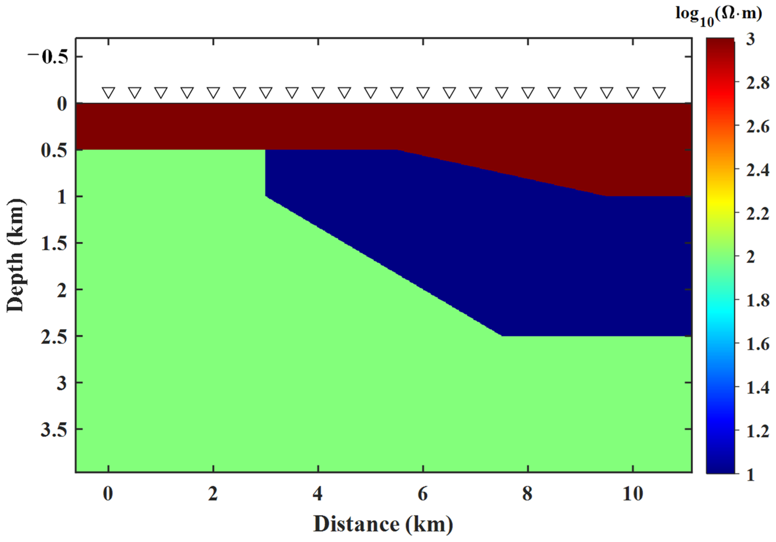
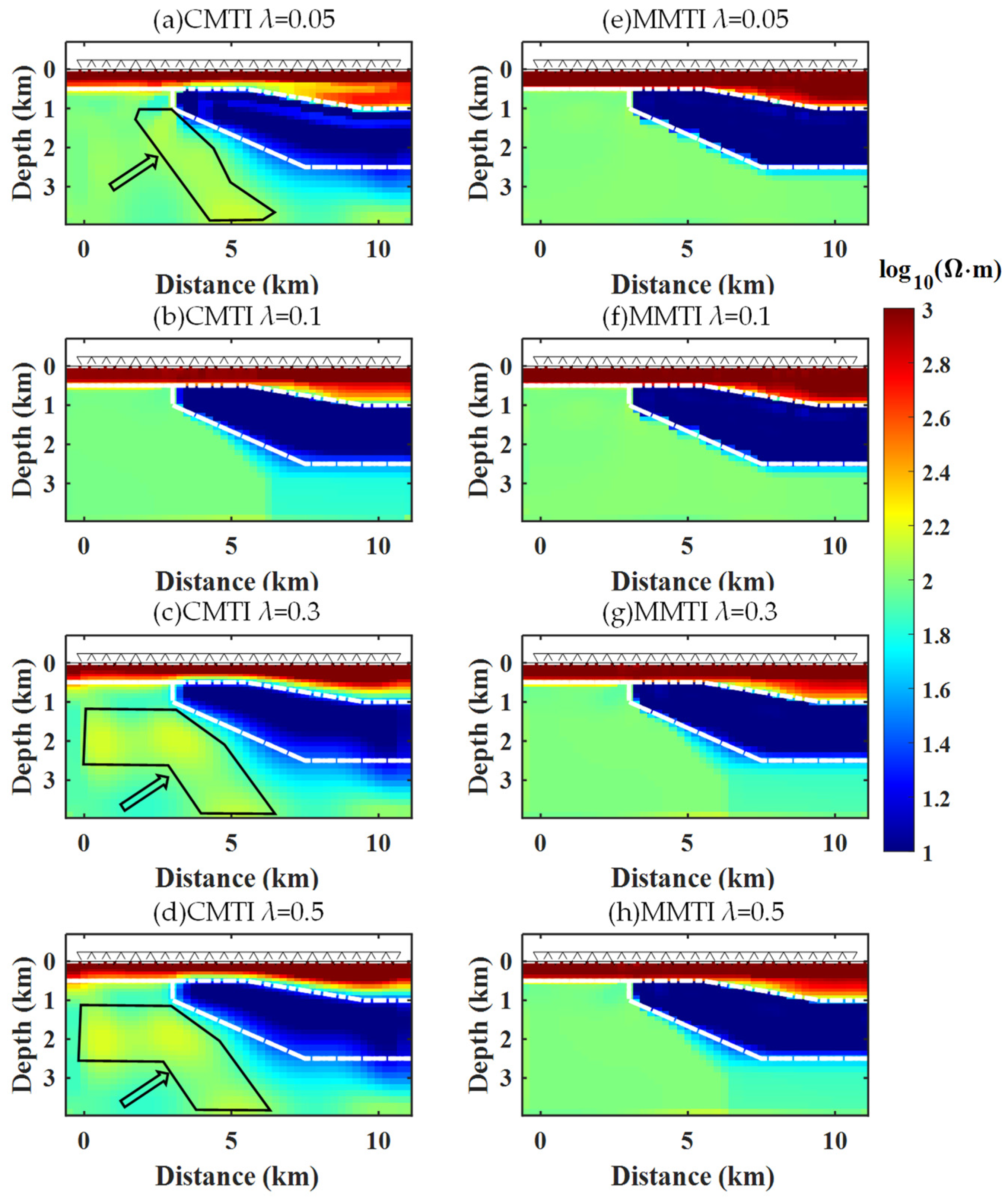
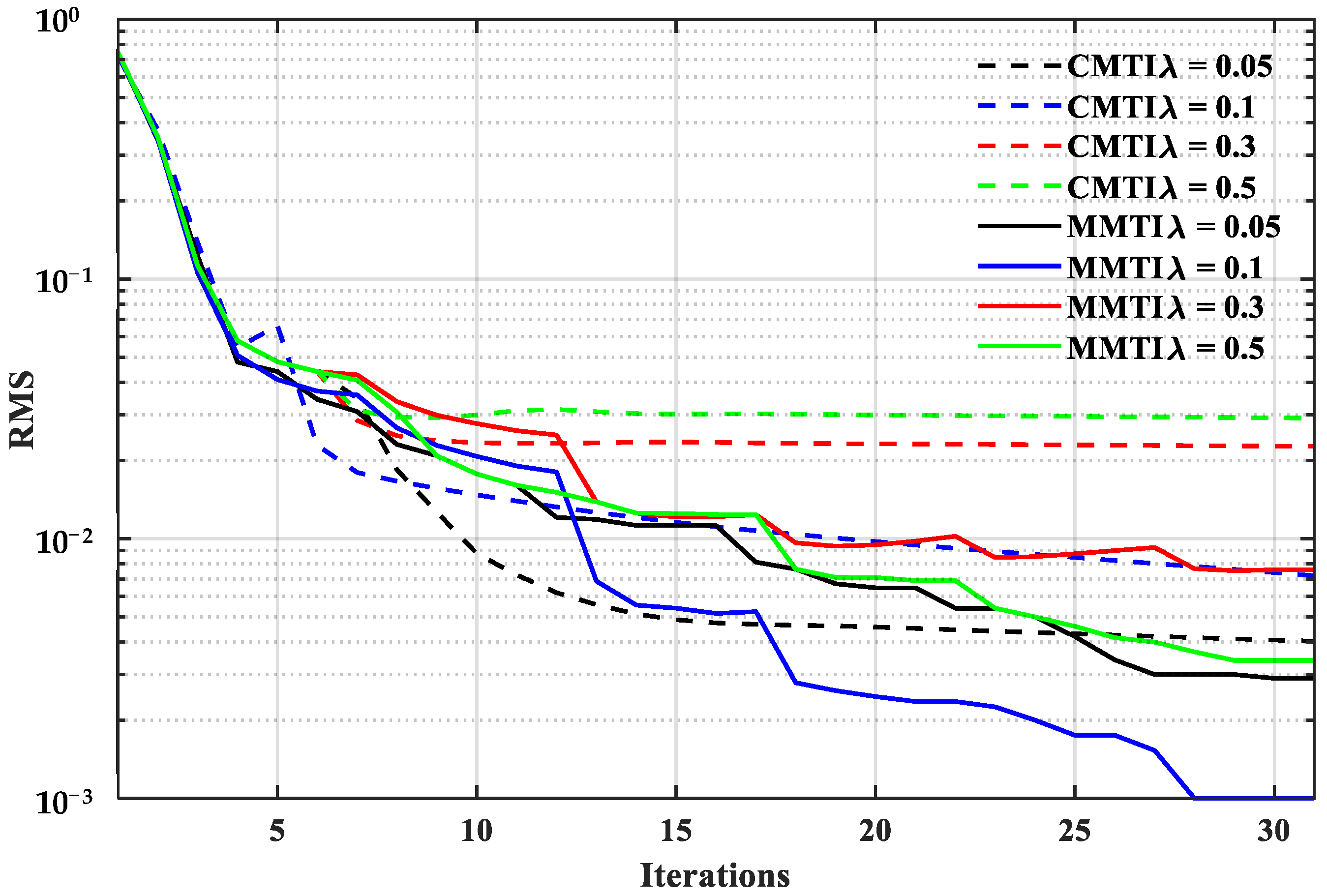
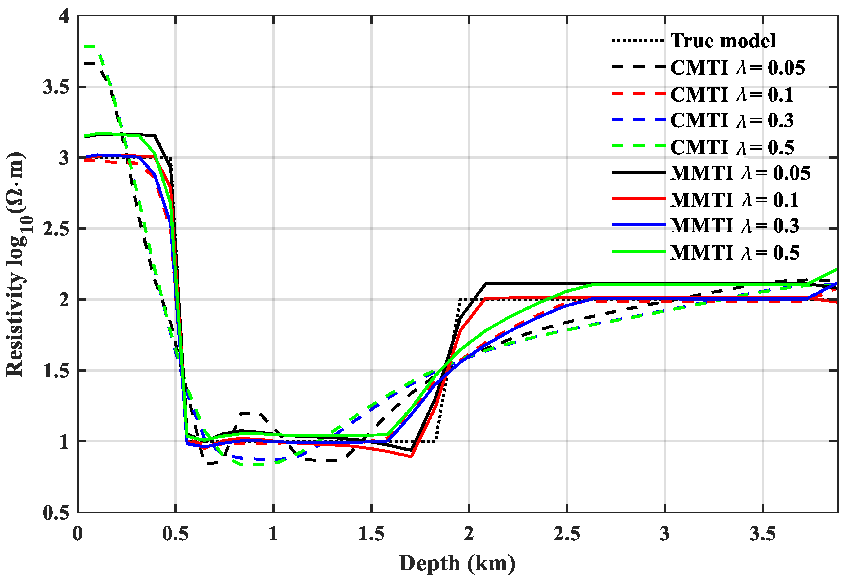
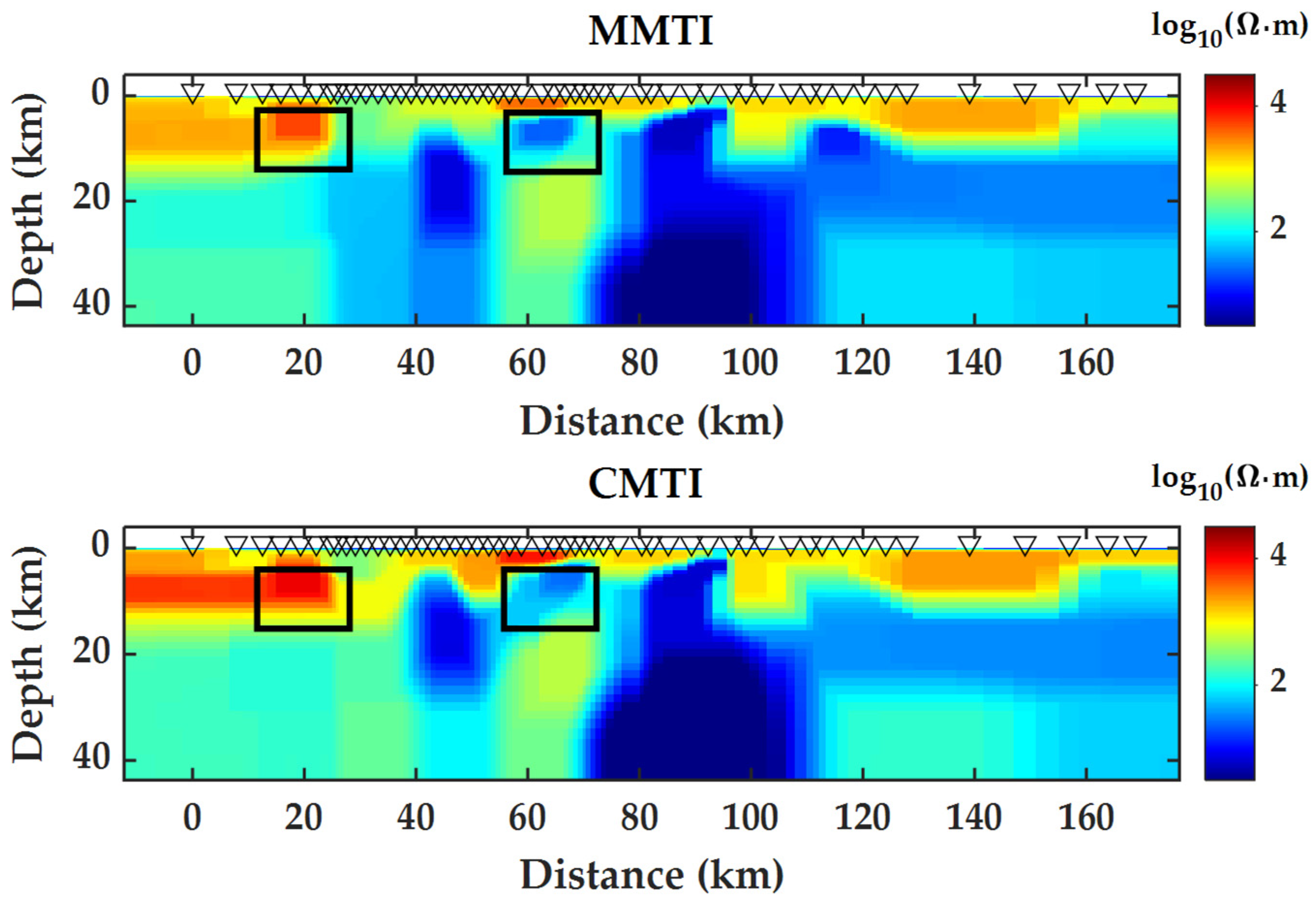
4.2. Wedge Model
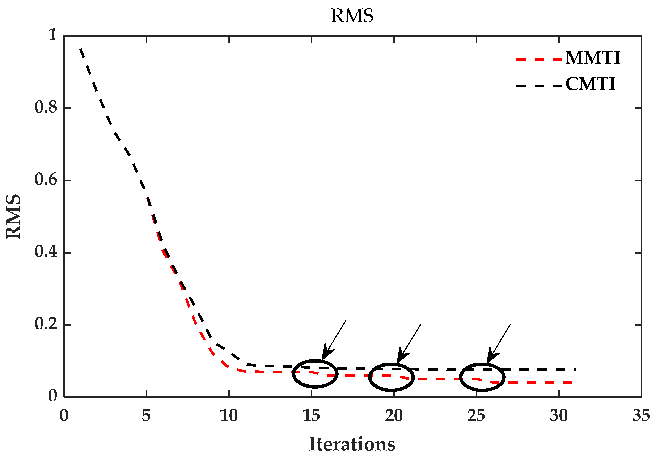
5. Field-Data Example
6. Conclusions
Author Contributions
Funding
Data Availability Statement
Conflicts of Interest
References
- Cagniard, L. Basic theory of the magneto-telluric method of geophysical prospecting. Geophysics 1953, 18, 605–635. [Google Scholar] [CrossRef]
- Tikhonov, A. On determining electrical characteristics of the deep layers of the Earth’s crust. Magn. Methods 1986, 73, 295–297. [Google Scholar]
- Jupp, D.L.; Vozoff, K. Two-dimensional magnetotelluric inversion. Geophys. J. Int. 1977, 50, 333–352. [Google Scholar] [CrossRef]
- Dittmer, J.K.; Szymanski, J. The stochastic inversion of magnetics and resistivity data using the simulated annealing algorithm. Geophys. Prospect. 1995, 43, 397–416. [Google Scholar] [CrossRef]
- Spichak, V.; Popova, I. Artificial neural network inversion of magnetotelluric data in terms of three-dimensional earth macroparameters. Geophys. J. Int. 2000, 142, 15–26. [Google Scholar] [CrossRef]
- Wang, H.; Liu, M.; Xi, Z.; Peng, X.; He, H. Magnetotelluric inversion based on BP neural network optimized by genetic algorithm. Chin. J. Geophys. 2018, 61, 1563–1575. [Google Scholar] [CrossRef]
- Pérez-Flores, M.A.; Schultz, A. Application of 2-D inversion with genetic algorithms to magnetotelluric data from geothermal areas. Earth Planets Space 2002, 54, 607–616. [Google Scholar] [CrossRef]
- Shaw, R.; Srivastava, S. Particle swarm optimization: A new tool to invert geophysical data. Geophysics 2007, 72, F75–F83. [Google Scholar] [CrossRef]
- Zhou, S.; Huang, Q. Two-dimensional sharp boundary magnetotelluric inversion using Bayesian theory. Chin. J. Geophys. 2018, 61, 3420–3434. [Google Scholar]
- Xiang, E.; Guo, R.; Dosso, S.E.; Liu, J.; Dong, H.; Ren, Z. Efficient hierarchical trans-dimensional Bayesian inversion of magnetotelluric data. Geophys. J. Int. 2018, 213, 1751–1767. [Google Scholar] [CrossRef]
- Conway, D.; Alexander, B.; King, M.; Heinson, G.; Kee, Y. Inverting magnetotelluric responses in a three-dimensional earth using fast forward approximations based on artificial neural networks. Comput. Geosci. 2019, 127, 44–52. [Google Scholar] [CrossRef]
- Liu, Z.; Chen, H.; Ren, Z.; Tang, J.; Xu, Z.; Chen, Y.; Liu, X. Deep learning audio magnetotellurics inversion using residual-based deep convolution neural network. J. Appl. Geophys. 2021, 188, 104309. [Google Scholar] [CrossRef]
- Constable, S.C.; Parker, R.L.; Constable, C.G. Occam’s inversion: A practical algorithm for generating smooth models from electromagnetic sounding data. Geophysics 1987, 52, 289–300. [Google Scholar] [CrossRef]
- Degroot-Hedlin, C.; Constable, S. Occam’s inversion and the North American Central Plains electrical anomaly. J. Geomagn. Geoelectr. 1993, 45, 985–999. [Google Scholar] [CrossRef]
- Siripunvaraporn, W.; Egbert, G. An efficient data-subspace inversion method for 2-D magnetotelluric dataREBOCC Inversion for 2-D MT Data. Geophysics 2000, 65, 791–803. [Google Scholar] [CrossRef]
- Smith, J.T.; Booker, J.R. Rapid inversion of two-and three-dimensional magnetotelluric data. J. Geophys. Res. Solid Earth 1991, 96, 3905–3922. [Google Scholar] [CrossRef]
- Tan, H.; Yu, Q.; John, B.; Wei, W. Three-dimensional rapid relaxation inversion for the magnetotelluric method. Chin. J. Geophys. 2003, 46, 1218–1226. [Google Scholar] [CrossRef]
- Mackie, R.L.; Madden, T.R. Three-dimensional magnetotelluric inversion using conjugate gradients. Geophys. J. Int. 1993, 115, 215–229. [Google Scholar] [CrossRef]
- Rodi, W.; Mackie, R.L. Nonlinear conjugate gradients algorithm for 2-D magnetotelluric inversion. Geophysics 2001, 66, 174–187. [Google Scholar] [CrossRef]
- Hu, Z.Z.; Hu, X.Y.; He, Z.X. Pseudo-three-dimensional magnetotelluric inversion using nonlinear conjugate gradients. Chin. J. Geophys. 2006, 49, 1111–1120. [Google Scholar] [CrossRef]
- Sasaki, M. An introspective account of L2 writing acquisition. In Reflections on Multiliterate Lives; Multilingual Matters: Bristol, UK, 2001; pp. 291–304, Saracino 2004a. [Google Scholar]
- Avdeev, D.; Avdeeva, A. 3D magnetotelluric inversion using a limited-memory quasi-Newton optimization. Geophysics 2009, 74, F45–F57. [Google Scholar] [CrossRef]
- Feng, D.; Su, X.; Wang, X.; Wang, X. A modified total variation regularization approach based on the Gauss-Newton algorithm and split Bregman iteration for magnetotelluric inversion. J. Appl. Geophys. 2020, 178, 104073. [Google Scholar] [CrossRef]
- Xie, J.; Cai, H.; Hu, X.; Long, Z.; Xu, S.; Fu, C.; Wang, Z.; Di, Q. 3-D Magnetotelluric Inversion and Application Using the Edge-Based Finite Element with Hexahedral Mesh. IEEE Trans. Geosci. Remote Sens. 2021, 60, 1–11. [Google Scholar] [CrossRef]
- Qin, C.; Liu, X.; Wang, X.; Sun, W.; Zhao, N. Three-dimensional inversion of magnetotelluric based on adaptive finite element method. Chin. J. Geophys. 2022, 65, 2311–2325. [Google Scholar]
- Mueller, J.L.; Siltanen, S. Linear and Nonlinear Inverse Problems with Practical Applications; SIAM: Philadelphia, PA, USA, 2012. [Google Scholar]
- Zhdanov, M.S.; Fang, S. Three-dimensional quasi-linear electromagnetic inversion. Radio Sci. 1996, 31, 741–754. [Google Scholar] [CrossRef]
- Newman, G.A.; Alumbaugh, D.L. Three-dimensional magnetotelluric inversion using non-linear conjugate gradients. Geophys. J. Int. 2000, 140, 410–424. [Google Scholar] [CrossRef]
- Esparza, J.R.F.; Treviño, E.G. 2-D Niblett-Bostick magnetotelluric inversion. Geol. Acta: Int. Earth Sci. J. 2010, 8, 15–30. [Google Scholar]
- Ye, T.; Chen, X.-B.; Yan, L.-J. Refined techniques for data processing and two-dimensional inversion in magnetotelluric (Ⅲ); using the Impressing Method to construct starting model of 2D magnetotelluric inversion. Chin. J. Geophys. 2013, 56, 3596–3606. [Google Scholar] [CrossRef]
- Tikhonov, A.N.; Glasko, V.B. Use of the regularization method in non-linear problems. USSR Comput. Math. Math. Phys. 1965, 5, 93–107. [Google Scholar] [CrossRef]
- Last, B.; Kubik, K. Compact gravity inversion. Geophysics 1983, 48, 713–721. [Google Scholar] [CrossRef]
- Portniaguine, O.; Zhdanov, M.S. Focusing geophysical inversion images. Geophysics 1999, 64, 874–887. [Google Scholar] [CrossRef]
- Grayver, A.V.; Kuvshinov, A.V. Exploring equivalence domain in nonlinear inverse problems using Covariance Matrix Adaption Evolution Strategy (CMAES) and random sampling. Geophys. J. Int. 2016, 205, 971–987. [Google Scholar] [CrossRef]
- Su, Y.; Yin, C.; Liu, Y.; Ren, X.; Zhang, B.; Qiu, C.; Xiong, B. 2D magnetotelluric sparse regularization inversion based on curvelet transform. Chin. J. Geophys. 2021, 64, 314–326. [Google Scholar]
- Hansen, P.C.; O’Leary, D.P. The use of the L-curve in the regularization of discrete ill-posed problems. SIAM J. Sci. Comput. 1993, 14, 1487–1503. [Google Scholar] [CrossRef]
- Haber, E.; Oldenburg, D. A GCV based method for nonlinear ill-posed problems. Comput. Geosci. 2000, 4, 41–63. [Google Scholar] [CrossRef]
- Zhdanov, M.S. Geophysical Inverse Theory and Regularization Problems; Elsevier: Amsterdam, The Netherlands, 2002; Volume 36. [Google Scholar]
- Chen, X.-B.; Zhao, G.-Z.; Tang, J.; Zhan, Y.; Wang, J.-J. An adaptive regularized inversion algorithm for magnetotelluric data. Chin. J. Geophys. 2005, 48, 937–946. [Google Scholar] [CrossRef]
- Jin, B.; Takeuchi, T. Lagrange optimality system for a class of nonsmooth convex optimization. Optimization 2016, 65, 1151–1166. [Google Scholar] [CrossRef]
- Bahreininejad, A. Improving the performance of water cycle algorithm using augmented Lagrangian method. Adv. Eng. Softw. 2019, 132, 55–64. [Google Scholar] [CrossRef]
- Alikhani Koupaei, J.; Firouznia, M. A chaos-based constrained optimization algorithm. J. Ambient. Intell. Humaniz. Comput. 2021, 12, 9953–9976. [Google Scholar] [CrossRef]
- Rockafellar, R.T. Augmented Lagrangians and hidden convexity in sufficient conditions for local optimality. Math. Program. 2022, 1–36. [Google Scholar] [CrossRef]
- Wu, W.; Yang, Y.; Zheng, H.; Zhang, L.; Zhang, N. Numerical manifold computational homogenization for hydro-dynamic analysis of discontinuous heterogeneous porous media. Comput. Methods Appl. Mech. Eng. 2022, 388, 114254. [Google Scholar] [CrossRef]
- de Groot-Hedlin, C.; Constable, S. Inversion of magnetotelluric data for 2D structure with sharp resistivity contrasts. Geophysics 2004, 69, 78–86. [Google Scholar] [CrossRef]
- Gholami, A.; Aghamiry, H.S.; Operto, S. Extended-space full-waveform inversion in the time domain with the augmented Lagrangian method. Geophysics 2022, 87, R63–R77. [Google Scholar] [CrossRef]
- Willoughby, R.A. Solutions of ill-posed problems (AN Tikhonov and VY Arsenin). SIAM Rev. 1979, 21, 266. [Google Scholar] [CrossRef]
- Hestenes, M.R. Multiplier and gradient methods. J. Optim. Theory Appl. 1969, 4, 303–320. [Google Scholar] [CrossRef]
- Luenberger, D.G.; Ye, Y. Linear and Nonlinear Programming; Springer: New York, NY, USA, 1984; Volume 2. [Google Scholar]
- Miele, A.; Moseley, P.; Levy, A.; Coggins, G. On the method of multipliers for mathematical programming problems. J. Optim. Theory Appl. 1972, 10, 1–33. [Google Scholar] [CrossRef]
- Tapia, R.A. Diagonalized multiplier methods and quasi-Newton methods for constrained optimization. J. Optim. Theory Appl. 1977, 22, 135–194. [Google Scholar] [CrossRef]
- Feng, D.; Liu, J.; Wang, X. MT finite element method forward modeling and inversion using irregular quadrilateral mesh of steep topography model. J. Cent. South Univ. 2018, 49, 626–632. [Google Scholar] [CrossRef]

| Method | Error (%) | RMS | Time (s) |
|---|---|---|---|
| Conventional | 9.57 | 0.0065 | 770.4180 |
| Multipliers | 7.41 | 0.0057 | 740.3230 |
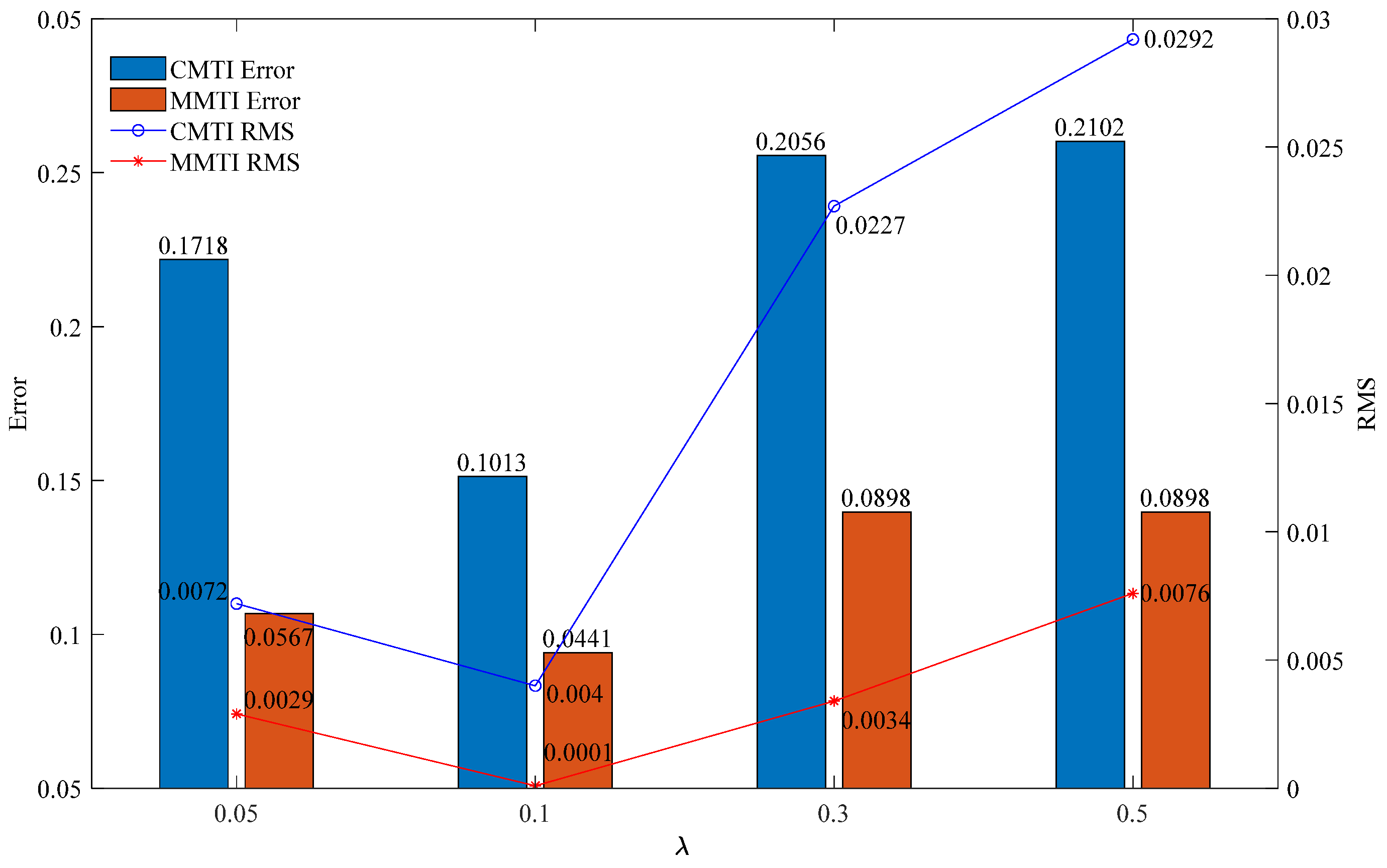
| Method | Regularization Parameter | Error (%) | RMS | Time (s) |
|---|---|---|---|---|
| Conventional | 0.05 | 17.18 | 0.0072 | 206.4840 |
| 0.1 | 10.13 | 0.0040 | 206.6550 | |
| 0.3 | 20.56 | 0.0227 | 208.2030 | |
| 0.5 | 21.02 | 0.0292 | 210.4520 | |
| Multipliers | 0.05 | 5.67 | 0.0029 | 204.4870 |
| 0.1 | 4.41 | 0.0001 | 201.8690 | |
| 0.3 | 8.98 | 0.0034 | 205.6320 | |
| 0.5 | 8.98 | 0.0076 | 208.5530 |
| Method | RMS | Time (s) |
|---|---|---|
| Conventional | 0.0760 | 1652.2350 |
| Multipliers | 0.0408 | 1456.3620 |
Publisher’s Note: MDPI stays neutral with regard to jurisdictional claims in published maps and institutional affiliations. |
© 2022 by the authors. Licensee MDPI, Basel, Switzerland. This article is an open access article distributed under the terms and conditions of the Creative Commons Attribution (CC BY) license (https://creativecommons.org/licenses/by/4.0/).
Share and Cite
Feng, D.; Su, X.; Wang, X.; Ding, S.; Cao, C.; Liu, S.; Lei, Y. Magnetotelluric Regularized Inversion Based on the Multiplier Method. Minerals 2022, 12, 1230. https://doi.org/10.3390/min12101230
Feng D, Su X, Wang X, Ding S, Cao C, Liu S, Lei Y. Magnetotelluric Regularized Inversion Based on the Multiplier Method. Minerals. 2022; 12(10):1230. https://doi.org/10.3390/min12101230
Chicago/Turabian StyleFeng, Deshan, Xuan Su, Xun Wang, Siyuan Ding, Cen Cao, Shuo Liu, and Yi Lei. 2022. "Magnetotelluric Regularized Inversion Based on the Multiplier Method" Minerals 12, no. 10: 1230. https://doi.org/10.3390/min12101230
APA StyleFeng, D., Su, X., Wang, X., Ding, S., Cao, C., Liu, S., & Lei, Y. (2022). Magnetotelluric Regularized Inversion Based on the Multiplier Method. Minerals, 12(10), 1230. https://doi.org/10.3390/min12101230