Abstract
Roll-front uranium deposits are ore mineralizations that occur in sandstones or arkoses downstream from redox fronts or reduced/oxidized geochemical barriers. They are often bounded above and below by impermeable shaly/muddy layers making them ideal for in-situ leaching exploitation. Several stochastic simulations were previously investigated either to characterize the ore grade distribution within roll-front type deposits, or for describing geological processes involved in their formation. This work suggests some modifications/improvements of conventional geostatistical algorithms for honoring hydrodynamic constraints that govern fluid flows in ore bearing layers. In particular, instead of using the classical Euclidian or curvilinear (for Sgrid) distance for computing the variogram, it is proposed to calculate the variogram accounting for the time of flight (TOF) of water particles down the streamlines together with available well data. Non-deterministic streamline-based methods seem to provide more accurate interpolation results and resource estimation compared to a traditional geostatistical approach when applied to roll-front deposits.
1. Introduction
Roll-front deposits are mineralizations that form at redox fronts downstream in permeable rocks [1]. Reduction reactions of aqueous uranium occurring at the redox front lead to precipitation of solid minerals. Oxygen-rich meteoric water continuously dissolves these solid minerals at the upgradient side of the roll-front, allowing the roll-front to advance downgradient. According to International Atomic Energy Agency (IAEA), roll-fronts have the following geometric characteristics: (i) a vertical crescent shaped formation that extends between two impermeable beddings with a distinctive elongated (C-shape) tongue; (ii) a planar horizontal sinusoidal front (or digitation) orthogonal to the groundwater flow direction [2]; (iii) the upstream part (back) of the accumulation has a sharp edge with oxidated species, while the downstream part (front) is diffusively extending into reduced rock [3].
Sandstone type deposits were the most common identified uranium resource type in 2020 (45% share for <USD 40/kgU price category) [2]. Roll-front deposits are highly suitable to be exploited using In-Situ Leaching technique (ISL), which is currently the main technology for producing uranium (accounting for 50% of World’s production in 2017). The ISL technology gives many countries the opportunity to increase their production. Kazakhstan, for instance, multiplied its annual production sixfold since 2009, now accounting for almost 40% of world’s total production [4]. Kazakhstan accounts for 15% of the global identified uranium resources, which makes it the second largest resource base after Australia, with more than half the resources produced by the ISL technique that can be attributed to the lowest category in terms of recovery costs at <USD 40/kgU [2]. Roll-front type deposits prevail throughout the world including USA, Mali, Nigeria, Czech Republic, Uzbekistan, etc. [5,6]. Moreover, apart from uranium, roll-fronts are sources of other minerals such as selenium (SE), molybdenum (Mo), rhenium (Re), vanadium (V), scandium (Sc), etc. [7].
Exploration of roll-front deposits is entirely based on systematic drilling, which starts with a series of widely spaced regular grids of wells placed along the redox front. The distance between wells is at first several kilometers, followed by a shortening to hundreds of meters upon encountering the mineralization. The final resource estimation is done on a 100 × 50 m or 50 × 20 m grid, when the geometry and content of the mineralization is determined to allow geotechnological mining operations [8].
Proper geomodeling techniques are highly required to accurately estimate ISL resources, the extraction profitability of the mineralization during the exploration stage, and to reduce exploitation costs with minimal number of wells and amount of leaching solution necessary during the production phase. The most conventional methods that are currently in use delineate the profitable exploitable ore body using interpreted GIS data [8], or apply geostatistical algorithms to estimate ore grade values at a regular grid covering the domain under consideration.
Several geostatistical approaches were investigated to model roll-front deposits containing uranium [8,9,10]. A 3D modeling technology based on the “Pluri-Gaussian Simulation” concepts has recently been used [9]. Conventional methods are subjective and their uncertainty cannot be reliably estimated, which leads many geostatistical approaches to use a pluri-gaussian simulation method [11] by picking the most probable model from several simulations. The epigenetic nature of the roll-front genesis is the reason for the uneven uranium grade distribution, creating intricate geometry of the concentrations which further complicates resource estimation process, and leading to noisy variograms that are usually dealt with Gaussian transformations [8].
Present geomodeling approaches hardly consider filtration and reactive transport processes that occurred during the formation of the roll-front uranium deposits. The main idea discussed in this paper is to integrate computational fluid dynamics into current geostatistical algorithms for accounting for such geological constraints.
Testing the accuracy of geological modeling is a challenge, since there is no way to reliably verify the accuracy of the resulting 3D models without drilling additional wells. Therefore, verification of the stochastic model is practically impossible without factual data. In this paper, the authors propose a technique to produce synthetic deposits, based on numerical simulation of hydrodynamics and chemical kinetics of precipitation/dissolution of mineral complexes during the deposit genesis. Notations and definitions are listed in Table 1.

Table 1.
Nomenclature.
2. Roll-Front Deposit Genesis Simulated by Reactive Transport Modeling
The uranium minerals accumulation process in roll-front deposits consists in two main phases (Figure 1).
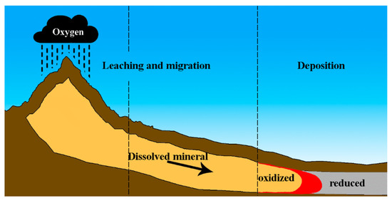
Figure 1.
Phases of uranium deposit genesis: migration and deposition.
Firstly, oxygen rich rainwater dissolves uranium complexes; driven by gravity, it migrates over a large period of time and distance throughout the permeable sandstones [12,13]. Secondly, upon reaching reducing environment/conditions, uranium together with others chemical elements (including Se, Mo, Re, Sc, Zn, Cu, Ag, Fe, As, Co, Ni, V, REE, etc.), precipitates due to redox reactions between U6+ and other elements/minerals with a low oxidation state (organic matter, pyrite, etc.). The main uraniferous minerals in Kazakhstan roll-front uranium deposits are coffinite and pitchblende. Kazakhstani ore deposits are hosted in sandy formations of the Eocene age. A continuous flow of oxygenated water re-dissolves precipitated uranium, which is then redeposited at a further distance downstream, as suggested by the U-Pb isotopic dating on ores which range mostly between 2 and 20 My. According to the authors [14], this reflects various remobilization events related to the continuous and still currently active roll-front evolution. In other words, the formation of roll-front deposits is a continuous cycle of redox reactions with dissolution, migration and precipitation of uranium complexes inside the porous medium. These redox zones create geochemical barriers that significantly reduce the migration properties of uranium and other minerals (such as selenium, molybdenum, rhenium and scandium [7]) thereby creating a roll-front deposit. Active deposits are affected by a constant flow of oxygen rich water that dissolves solidified minerals and redeposits them in the direction of groundwater flow. At a stable state redeposition does not occur due to the absence of oxidizer in groundwater.
According to Romberger [15] uranium can migrate in 43 various complexes including sulfates, carbonates, phosphates, chlorides and fluorides, although U4+ can be neglected due to its low solubility. The solubility of these complexes and their precipitation properties may dependent on pressure, temperature, oxidation state and pH. While pressure and temperature are stable environmental factors, Eh and pH depend on chemical reactions occurring at the geochemical barriers.
Oxidized dissolution of stoichiometric mineral oxides can be described by the following global chemical reactions [7]:
Maximova [7] proposes to generalize them into the following set of half reactions for uranium (U):
Electron containing compounds precipitate dissolved uranium. On the contrary, oxygenated waters redeposit uranium crystals by dissolving them back into mobile complexes. The electron availability is a result of the redox reactions between oxygen rich water and reductant occurring at the geochemical barrier.
A simplified model of the process of roll-front genesis to generate a realistic spatial distribution of uranium deposit has been used on the basis of previous work [14], in which authors conducted numerical experiments to identify reaction rate constants based on available empirical experimental data. Similar experiments were conducted in order to generate a synthetic deposit. Dissolved minerals along with an oxidant are injected from one side into a 270 × 450 × 60 m box domain (Figure 2). Oxygenated fluid containing dissolved minerals enters the box from one side (inlet), reacts with the compounds hosted within the box, and leaves from the opposing side (outlet). The other lateral sides of the box are considered as impermeable.
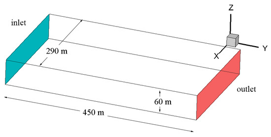
Figure 2.
Simulation domain with inflow side (green), and outflow side (red).
Simulation of the synthetic roll-front deposit is conducted within the following steps. Firstly, nonhomogeneous distribution of filtration coefficient (permeability) is generated within the calculation grid inside the domain. A continuous delivery of oxygen and uranium is provided until the maximum concentration of uranium reaches values comparable to those observed in real deposits (0.03% [12]). When the desired concentration is reached, the delivery of uranium is stopped to let the mineral concentration be redeposited, accumulated and acquire a roll-front shaped form somewhere downstream.
The following assumptions are made while constructing a system:
- all fluids are considered as incompressible;
- the diffusive transport of the mineral is much lower in comparison with convective transport;
- the values of concentration of minerals that are affected by reactions are very low, therefore porosity is taken as constant;
- fluid flow inside the porous and permeable domain is modeled based on the Darcy equation, the mass conservation principle, and the Mass Action Law [16].
The initial distribution of the permeability was set as idealistic and heterogeneous (Figure 3) to force distinctive sinusoidal shape of the deposit.
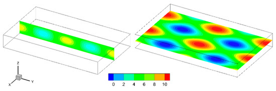
Figure 3.
Permeability distribution measured in meters per day.
Boundary conditions for pressure were set as no-flow on lateral boundaries of the domain, and based on hydraulic head on inflow and outflow sides depending on the height difference between inlet and outlet equal to 2 m (Figure 2). The reductant is taken as abundant throughout the domain.
Apart from the reductant, the initial conditions for all concentrations inside the domain were set to zero. During the simulation, dissolved mineral concentrations were set to zero upon reaching desired maximum concentration of 0.03%, which is generally considered as profitable to be exploited [12].
Consequently, synthetic three-dimensional models of roll-front deposits were generated for the purposes of verification and comparison of geostatistical methods (Figure 4 and Figure 5).
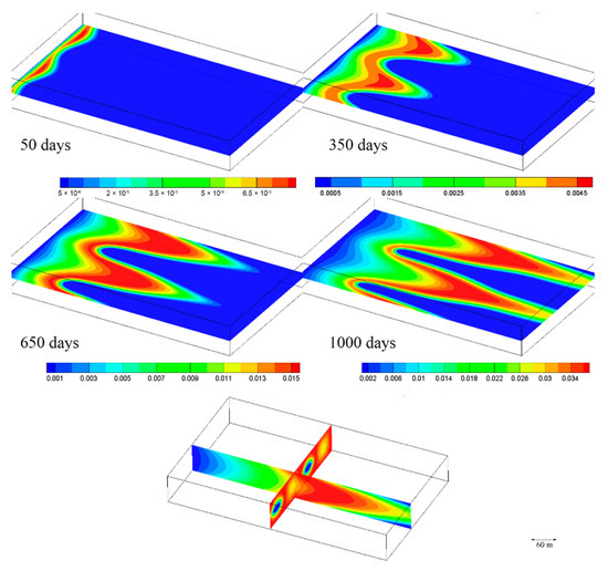
Figure 4.
Z-axis slice depicting the change in solid mineral concentration over 1000 simulated days (i.e., about less than 3 years) with varying legend (in percent) to show small concentration at initial stage.
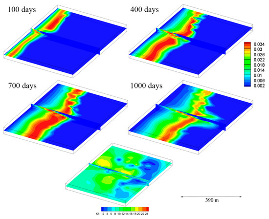
Figure 5.
Deposit genesis over time through a heterogenous porous media.
Further simulation has been conducted on a domain with filtration properties distribution taken from a real deposit in Southern Kazakhstan (Figure 5) to generate a second deposit.
3. Streamline-Based Stochastic Method and Resource Estimation of Roll-Front Uranium Deposits
Well logging is currently the single reliable method to measure solid mineral concentrations and is used as an input data for geostatistical methods. The goal of geostatistical methods is to determine the spatial distribution and concentration of minerals in the inter-well space. Roll-fronts are classified as epigenetic mineral deposits, i.e., their genesis occurred after creation of the hosting environment (mainly Eocene sandy formations for uranium deposits in Kazakhstan). Their structure and geometry results in preferential flow paths and fingering patterns typical of solute transport processes through a porous media with unstable fingering fronts (non-Fickian flow transport). Therefore, it is more difficult to apply traditional stochastic methods used to interpolate permeability or porosity data due to the lack of apparent horizontal anisotropy inherent to the sedimentary rocks.
The nature of roll-front formation is dictated by the hydrodynamics of infiltration process. Intuitively, accounting for the hydrodynamic properties of the stratum in geostatistical calculation should increase the accuracy of geomodelling processes.
3.1. Streamline-Based Stochastic Method
The suggested approach used in this work is based on streamlines calculated from filtration velocity vectors; streamlines are a set of curves that materializes the particle trajectory tangent to the flow velocity vectors in a selected domain. Streamlines are a widely used technology in multi-phase flow transport modeling in oil and gas reservoirs since the 2000s [17,18,19,20], but few uses in mineral resources applications were reported in the literature. It is classical to parametrize the streamlines by their proper time, referred as the time of flight (TOF), defined as the required time by a fluid molecule to travel from the injection well/point through the medium along the streamline.
Applied to resource estimation and geomodelling of deposits, the general formula of an estimation type geostatistical method includes the determination of weight (λi) assignment to hard datapoint (well observations) located at xi with a concentration value Z(xi) to estimate a concentration Z*(x) at a point of interest x (notations and definitions are shown for all consequent equations are shown on Table 1):
The chosen algorithm to determine and assign weight to hard data points will affect the accuracy of any method at hand. Inverse distance methods use specific coefficients to determine the exponential curve of correlation over distance, whereas in kriging-based methods a variogram function is calculated over a given hard data.
The aim of this work is to amend the ordinary kriging algorithm to use streamlines as guiding lines to find influencing nodes and calculate time of flight along these nodes to assign weights. In other words, the streamline-based kriging method is an ordinary kriging in a Riemannian (or non-Euclidian) space in which distances are defined by the TOF calculated along the streamlines (equivalent of the timelines). Streamline-based Kriging interpolation will therefore consist of the following steps: (i) the construction of the streamlines through the medium after solving the flow transport equation; (ii) the use of the substitute distances with TOF for Kriging calculations; (iii) classical calculation using conventional kriging algorithm but using the TOF distance (flow time difference) instead of Euclidian distance (Figure 6). In order to construct streamlines, the following steps are necessary: (a) calculation of the pressure field based on the filtration properties from hard data; (b) calculation of the velocity field based on Darcy’s Law; building of streamlines; (c) estimation of the time of flight along the streamlines.
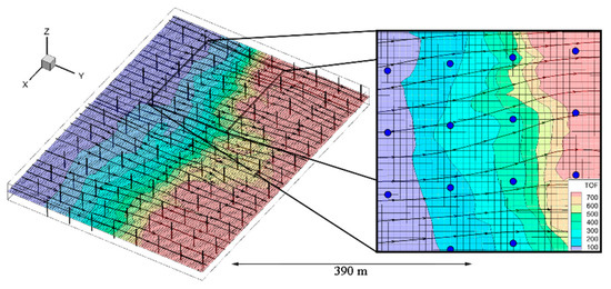
Figure 6.
Calculated streamlines and value of TOF throughout the domain.
The pressure field is calculated based on known length between inflow and outflow sides of the geological block under consideration, as well as the average permeability and the groundwater velocity, while the velocity is calculated based on the Darcy’s Law and the incompressible continuity equation:
The hydrodynamic pressure is determined by the following equation:
The streamlines are calculated using Pollock’s method [21] with a technique suggested in [22] firstly for each known hard data point (well logging data) along each well and then for each node in the grid, followed by the calculation of the time of flight for each streamline. The issue is to guarantee that each streamline will pass through hard data point. However, this is almost impossible if the starting point for each streamline is assigned to the inflow side of the domain. In this case, streamlines will almost certainly split or drift together following the iso-pressure surfaces. To solve this, we chose the starting point for each streamline at each hard data point along the well first downstream, then we apply a reverse upstream tracking algorithm. Resulting downstream and upstream streamlines are merged and the time of flight is recalculated (Figure 7).
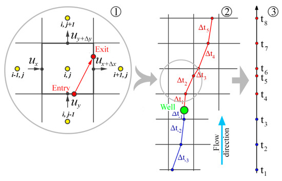
Figure 7.
(1) Streamline calculation according to Pollock’s method; (2) streamline calculation downstream and upstream from well; (3) upstream and downstream streamlines merging.
The same operation can be done for each node of the source grid. Depending on the velocity field (calculated from the pressure field which in turn is a result of the permeability assigned to the domain) the same value of time of flight will occur at different distances along the streamlines. Connecting points of each streamline with the same time of flight, allows the construction of a regular curved grid that respects the hydrodynamic properties of the domain (see Figure 8). This deformed non-Euclidian 2D or 3D space will be used to compute distances for estimating variograms or performing kriging.
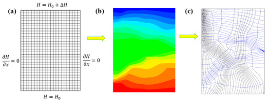
Figure 8.
(a) Source calculation grid; (b) calculated pressure field; (c) streamlines and orthogonal time of flight iso-surfaces.
In a conventional approach, iteratively, for each point where an estimation or a simulation is performed, a set of hard data points is gathered within the radius of a search ellipsoid, the shape of which depends on a selected anisotropy as illustrated in Figure 9.
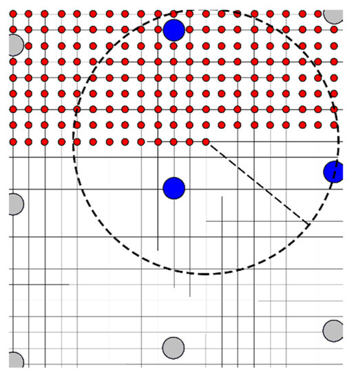
Figure 9.
Searching for influencing points.
In the proposed approach, a similar operation is conducted for each grid node in the domain under consideration. However, the points are searched within the TOF value difference and along the calculated streamlines (Figure 10). The assumption is that, due to epigenetic and hydrodynamic nature of deposit genesis, points connected by streamlines (or closer along a streamline) should have more influence in the estimation process. In other words, two points are close if they are connected by a groundwater flow streamline, and their distance is proportional to their TOF value difference.
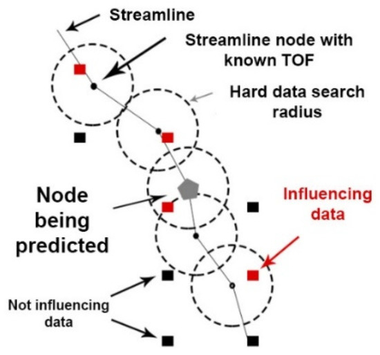
Figure 10.
Time of flight assigned to hard data found along the streamline is used as a distance parameter for calculating the variogram, while influencing points are searched within given TOF distance from the streamline.
The variogram is calculated over each streamline using the time of flight instead of the Euclidian distance:
where γ(l) is a variogram at the TOF distance l, N(l) is the number of nodes separated by time difference l and τ(x) is a time of flight of node x over a streamline that passes through it.
Weights are determined for each hard data node found along the streamline where C is a correlogram calculated as C(l) = σ2 − γ(l) (stationary case):
or by solving the resulting kriging system in moving neighborhoods; this method also gives an estimated variance for each estimate .
3.2. Implementation of the Streamline-Based Stochastic Method
A set of wells are drilled into previously generated synthetic roll-front deposit to test the proposed method (Figure 11). Hard data is collected from each well and is used as an input data for the method. True grade distribution within an exploited ore deposit will be used to estimate the error of the proposed method.
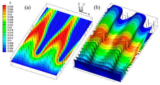
Figure 11.
Exploratory wells are put through a synthetic deposit. (a) Slice through z-axis; (b) iso-surfaces by pressure values in 3D.
A conventional kriging is used to populate the nodes with permeability values based on well log data. Pressure field, velocity field and resulting streamlines are calculated in the domain based on filtration properties of the stratum with thickness typically around 40 m (Figure 12).
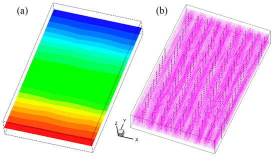
Figure 12.
(a) Pressure field with a slice through z-axis; (b) streamlines.
Streamline-based interpolation of well data resulted in uranium distribution along with results of ordinary kriging interpolation made using the SGeMS software are shown on Figure 13.
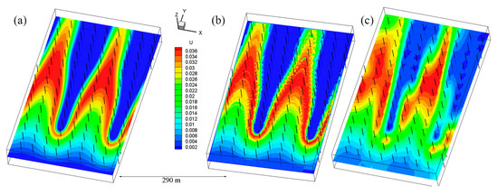
Figure 13.
Interpolation results where (a) true synthetic deposit; (b) streamline-based interpolation; (c) ordinary kriging-based interpolation with SGeMS software.
A synthetic deposit was generated based on the filtration data measured on a real geological block from a roll-front type deposit located in Southern Kazakhstan. The results obtained when applying the streamline-based stochastic method as well as the conventional kriging are shown on Figure 14.
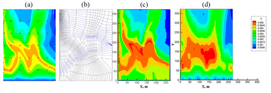
Figure 14.
Interpolation results based on real filtration data (a) synthetic deposit; (b) streamline and time of flight-based grid; (c) streamline-based interpolation; (d) ordinary kriging-based interpolation with SGeMS software.
3.3. Resource Estimation and Comparison
Resources are estimated based on the following formula:
where is the total resources in kilograms, is the concentration (in percent %) of uranium in node/cell i, is the density, taken at 1700 kg/m−3, is the porosity, and is the volume of cell number i.
Figure 15 compares the resource estimation obtained using classical kriging with the proposed streamline method. Two separate estimations were conducted: the total ISL resources, and the so-called balance resources, where nodes with concentration profitable to extract (taken as higher than 0.03%) were only accounted for. This is done because the main accumulation of resources is at the roll-front line itself, and “unbalanced” ore with small concentrations is usually deemed to be unprofitable and cut off from the resources [8].
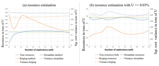
Figure 15.
Comparison in resource estimation (left vertical axis) and square root of dispersion variance (right vertical axis) between streamline-based stochastic method and ordinary kriging where (a) total in-situ resources in tons from all nodes; (b) recoverable resources in tons with concentration higher than 0.03%.
Total resources in the studied domain are equal to 1393 tons of U, whereas the total resources with profitable to extract U (taken as U higher than 0.03%) amounted to less than 688 tons of U. In the first case, the kriging method significantly overestimated U resources, whereas in the second case the kriging method underestimated total mineral content of the deposit. In both cases the streamline method has shown higher accuracy compared to the kriging method. For a particular case, with 80 exploratory wells, the streamline-based stochastic method estimated 694.10 ± 0.05 tons of uranium, while ordinary kriging calculated 579.77 ± 0.05 tons of uranium. The ordinary kriging algorithm demonstrated a significant improvement with the rise of exploratory well number, whereas the streamline-based approach displayed a sharp rise in accuracy with a lower number of exploratory wells. At the number of exploratory wells equal to 28, a spike in accuracy of conventional kriging is observed due to wells being positioned at high grade locations.
Nodes with values below cut-off are discarded during estimation since the concentration is too low and unprofitable. For the particular case of 53 exploratory wells, resources were estimated for various cut-off values. Grade cut-off curves are shown on Figure 16, where both proposed streamline and kriging methods show similar in-situ reserves for the quantity of metal against cut-offs. Kriging seems to overestimate the in-situ reserves for small cutoffs, and underestimate them for cut-off greater than the operation cut-off at 0.3‰ U (Figure 16a), with the average grade of the produced tonnage being underestimated in every case (Figure 16b).
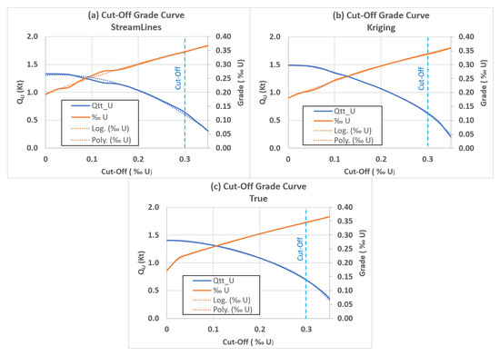
Figure 16.
Grade cut-off diagrams with resources (blue) and grades (orange) over cut-offs ranging from 0 to 0.35 ‰U, together with fitted trend lines (dotted) and exploitation cut-off at 0.3‰U (blue vertical dashed line) for (a) streamline-based proposed method; (b) kriging method; (c) true resources taken from the simulated deposit.
In Figure 16, the theoretical quantity of metal (/grade () vs. cut-off curves have been fit using a mean squared errors (MSE) method given the following equations:
Grade values and resource estimation for the average case of 53 exploratory wells are shown together with uncertainty estimation bars on Figure 17. Error bars were calculated as the absolute difference between the estimated and the true values on each cell, then as a sum on all cells satisfying the constraints used to calculate the cut-off curve. Again, for lower grade cut-offs the streamline-based proposed method shows a slightly higher accuracy for grade values as well as for resources, while for higher cut-offs (specifically larger than 0.1) kriging appears to be at the same level or even better than proposed approach.
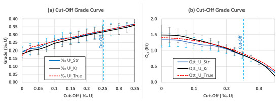
Figure 17.
Grade cut-off curves with (a) grades and uncertainty; (b) quantity of U and uncertainty for streamline-based method (blue) and kriging method (black) and synthetic deposit (red, dashed).
An important remark can be made regarding the operational cut-off used (in the case fixed at 0.3‰U) for selecting blocks for lixiviation. As shown on grade vs. cut-off curves (Figure 16c) the average produced grade is about 0.35‰U, much higher than the operational cut-off at 0.3‰U. If the objective of the mining producer is to produce an average lixiviate at a grade of 0.3‰U, a cut-off at 0.2‰U can be rather chosen (Figure 16c), increasing the in-situ reserves quantity of metal from 688 to 1084 t U (i.e., an additional 396 t U). Assuming an average prize at USD 130, it represents an additional in-situ value of $ USD 51.48 M. Of course, exploitation cost increase when cut-off grades are lower because it implies larger cell numbers to be lixiviated, so larger number of exploitation wells, and larger quantity of lixiviate. However, these curves demonstrate that case dependent optimum cut-off grades should be investigated according to the economic situation of deposits in order to maximize the profit.
An additional estimation has been conducted on a synthetic deposit generated based on the data from a real deposit in Southern Kazakhstan (Figure 18).
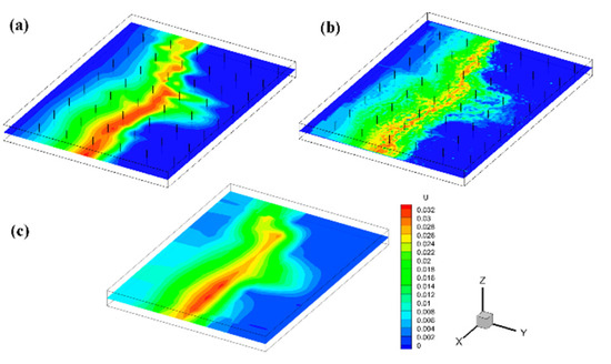
Figure 18.
Interpolation results where (a) true synthetic deposit based on real permeability data from the industry; (b) streamline-based interpolation; (c) ordinary kriging-based interpolation.
Total resources in the studied domain are equal to 357 tons of U with a cutoff of 0.03% (Figure 19). Similar to the first case, the kriging method overestimated U resources, whereas the streamline-based approach underestimated U reserves. Overall, the streamline method has shown higher accuracy as compared to the kriging method. For a particular case, with 48 exploratory wells, for true resources equal to 357 tons, streamline-based kriging underestimated resources to 346 tons, whereas ordinary kriging overestimated resources to 380 tons. The ordinary kriging algorithm demonstrated a significant improvement with the rise of exploratory well number, while streamline-based method displayed a sharp rise in accuracy with a lower number of exploratory wells.
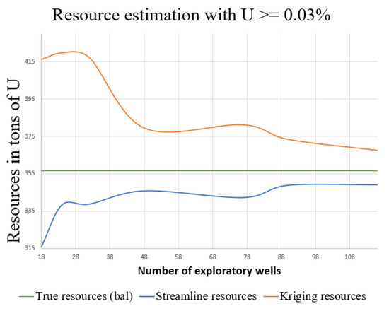
Figure 19.
Comparison in resource estimation between streamline-based stochastic method and ordinary kriging for a synthetic deposit generated based on the data from a real deposit.
4. Discussion
Figure 15 and Figure 16 demonstrate that the streamline-based interpolation approach provides qualitatively better results as compared to the conventional kriging method. Qualitatively, the roll-front structure is preserved due to hydrodynamic nature of interpolation.
Additionally, for qualitative analysis, an error estimation has been carried out as shown on Figure 20. Maximum errors for each exploratory well amount were calculated as a maximum difference between values obtained from the synthetic deposit and respective algorithm of geostatistics. Similarly, average errors were calculated as an average difference between values obtained from the synthetic deposit and respective algorithm of geostatistics. Quantitatively, with an increased number of wells the maximum error of the ordinary kriging algorithm sharply decreases, while streamline-based interpolation preserved an initial irreducible value. Higher values of maximum errors for streamline-based interpolation are observed at the upstream part of the domain (the start of streamlines). Average errors for streamline-based kriging are lower as compared to the ordinary kriging with a different numbers of exploratory wells.
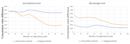
Figure 20.
Errors in resource estimation comparison between streamline-based stochastic method and ordinary kriging where (a) maximum error from all nodes; (b) average error from all nodes.
The ordinary kriging algorithm, due to its smoothness, provided a diffusive end result, whereas the streamline-based interpolation in some cases provides better accuracy at the geochemical barrier/front itself. As shown in Figure 13, when nodes containing profitable mineral concentration are taken into account (cut-off of 0.03%), the streamline-based interpolation achieves better accuracy in terms of resource estimation.
One of the disadvantages of the streamline-based interpolation methods is that sufficient hard data/knowledge (such as geological formation, permeability of layers, etc.) of the deposit is required in order to be able to build a realistic flow model for computing the streamlines.
An advantage of the streamline-based methods is that other geostatistical methods in addition to kriging, such as various simulation techniques including SGS, multi-Gaussian, turning bands, etc., can be implemented using the TOF instead of the classical Euclidian spatial distance. An assumption, however, is that permeability field in the domain is constant at all times. This might be true due to epigenetic nature of roll-front formation, i.e., hosting environment has been established before the infiltration process begun. It is difficult to estimate past permeability, which if it differs might affect the estimation result.
Streamline-based kriging might only perform well on idealized synthetic deposits. Currently, kriging together with other methods of geostatistics are used to model uranium deposits. However, there is no reliable method to verify the accuracy of these methods, which would require a full MRI scan of the stratum. Granted, usage of the synthetic data cannot prove that one or the other method will be accurate in real world conditions. Presented in this paper is an alternative approach to at least have a preliminary verification method. In a way the method itself is ordinary kriging in a Riemann space defined by streamlines. Streamlines themselves provide additional information, that can increase the accuracy of conventional methods. As mentioned before, a major assumption of the paper is that for epigenetic deposits the hosting environment has formed before the inflow of minerals. Hydrodynamic conditions might have been different at various points in time, which might lead to streamline-based kriging being less accurate than ordinary geostatistical calculations. This can possibly be solved if an additional information is provided to the method itself from the available historical information. Initial homogeneity of the reduced environment was assumed to exclude the factor of heterogeneity of the reduced environment. The method itself is based on streamlines, which were obtain from Darcy’s law. Darcy’s law, however, does account for heterogeneity of the medium. Reactive transport simulations are critical for the streamline-based method, but may be used as a preliminary verification instrument.
5. Conclusions
The research work described in this paper consists of two phases. Firstly, a reactive transport model was used to simulate the roll-front genesis in order to create synthetic uranium deposits. Secondly, a new geostatistical method, referred as the streamline-based kriging method, was developed to take into to account the hydrodynamic nature of roll-front deposit formation. The new method was tested on synthetic deposits in order to estimate its qualitative and quantitative advantages. Various geometries of underlying host environment were used to generate synthetic deposits and to test stochastic methods. For better evaluation, methods were tested with varying available well log data. Results show that in terms of error, as compared to conventional estimation algorithm of kriging, geological modeling of uranium roll-front deposits based on streamline simulation provided improved resource estimation with lower average error.
The method can be applied for an epigenetic deposit which formed through the infiltration process. Variogram calculation along the streamlines provides additional information for more precise weight assignment. Additionally, other available geostatistical methods can be amended in a similar way to account for the hydrodynamics underlying deposit genesis.
Generally speaking, the simulation methods used here to test different estimation methods have another advantage: they can be profitably used as a training simulator to teach professionals or students how to select blocks in the lixiviation technology in order to optimize the production.
Further work has to be done to verify the technique with real case deposits, as well as to modify other stochastic methods to use streamline simulation as an additional tool. This new approach opens the door for future implementations of the geostatistical simulation toolbox on non-Euclidian distance problems where distances can be deduced from the resolution of a flow transport model.
Author Contributions
Conceptualization, D.A.; methodology, D.A. and A.K.; software, D.A.; validation, D.A. and M.T.; formal analysis, D.A. and A.K.; investigation, D.A.; resources, A.K. and M.T.; data curation, A.K.; writing—original draft preparation, D.A.; writing—review and editing, D.A.; visualization, D.A.; supervision, A.K.; project administration, M.T.; funding acquisition, M.T. and A.K. All authors have read and agreed to the published version of the manuscript.
Funding
The research was funded by the Ministry of Education of Kazakhstan, projects No AP08051929 and AP09260105.
Data Availability Statement
The data are not publicly available for reasons of confidentiality.
Acknowledgments
The idea was suggested by ENSG in Geomodeling of Lorraine University Guillaume Caumon. A number of ideas were suggested by Jean-Jacques Royer in order to improve the final version of the paper. The work was conducted at Satbayev University, Al-Farabi Kazakh National University and Laboratory of Georessources of Lorraine University, Nancy, France.
Conflicts of Interest
The authors declare no conflict of interest.
References
- Adams, S.S.; Cramer, R.T. Data-process-criteria model for roll-type uranium deposits. Geol. Environ. Sandstone-Type Uranium Depos. 1985, 16, 383–399. [Google Scholar]
- OECD-NEA; IAEA. Uranium 2020: Resources, Production and Demand; No. 7551; Nuclear Energy Agency and the International Atomic Energy Agency: Vienna, Austria, 2020; p. 479. [Google Scholar]
- Royer, J.J. Are World Uranium Resources Log-Normally Distributed? In Quantitative and Spatial Evaluations of Undiscovered Uranium Resources; IAEA TECDOC 1861: Vienna, Austria, 2018; pp. 173–202. [Google Scholar]
- Boytsov, A. Sustainable development of uranium production: Status, prospects, challenges. In Proceedings of the International Symposium on Uranium Raw Material for the Nuclear fuel Cycle: Exploration, Mining, Production, Supply and Demand, Economics and Environmental issues (URAM-2018), IAEA, Vienna, Austria, 25–29 June 2018; pp. 49–50. [Google Scholar]
- Dahlkamp, F.J. Uranium Deposits of the World (Asia); Springer: Berlin/Heidelberg, Germany, 2009; p. 492. [Google Scholar]
- Tarkhanov, A.B.; Bugrieva, Y.P. Krupneishye Uranovye Mestorozhdeniya Mira [Largest Uranium Deposits of the World]; Minerals Journal under All-Russian Research Institute of Mineral Raw Materials: Moscow, Russia, 2012; p. 118. [Google Scholar]
- Maksimova, M.F.; Shmariovich, Y.M. Plastovo-Infiltratsionnoye Rudoobrazovanie [Stratum-Infiltration ore Formation]; Nedra: Moscow, Russia, 1993; p. 160. [Google Scholar]
- Abzalov, M.; Drobov, S.; Gorbatenko, O.; Vershkov, A.; Bertoli, O.; Renard, D.; Beucher, H. Resource estimation of in situ leach uranium projects. Appl. Earth Sci. 2014, 123, 70–85. [Google Scholar] [CrossRef]
- Renard, D.; Beucher, H. 3D representations of a uranium roll-front deposit. Appl. Earth Sci. 2012, 121, 84–88. [Google Scholar] [CrossRef]
- Petit, G.; Boissezon, H.; Langlais, V.; Rumbach, G.; Khairuldin, A.; Oppeneau, T.; Fiet, N. Application of Stochastic Simulations and Quantifying Uncertainties in the Drilling of Roll Front Uranium Deposits. Quant. Geol. Geostat. 2012, 17, 321–332. [Google Scholar]
- Armstrong, M.; Galli, A.; Beucher, H.; Le Loc’h, G.; Renard, D.; Doligez, B.; Eschard, R.; Geffroy, F. Plurigaussian Simulation in Geosciences, 2nd ed.; Springer: Berlin, Germany, 2011; p. 176. [Google Scholar]
- Poezhaev, I.P.; Polinovskiy, K.D.; Gorbatenko, O.A. Uranium Geotechnology: A Training Manual; Insitute of High Technology Kazatomprom: Almaty, Kazakhstan, 2017; p. 327. [Google Scholar]
- Brovin, K.G.; Grabovnikov, V.A.; Shumilin, M.V.; Yazikov, V.G. Prognoz, Poiski, Razvedka I Promyshlennaya Ocenka Mestorozhdeniy Urana Dlya Otrabotki Podzemnym Vyshelachivaniyem [Forecast, Search, Exploration and Industrial Estimation of Uranium Deposits for Production with in-situ Leaching Method]; Gylym: Almaty, Kazakhstan, 1997; p. 384. [Google Scholar]
- Aizhulov, D.; Shyakhmetov, N.M.; Kaltayev, A. Quantitative model of the formation mechanism of the roll-front uranium deposits. Eurasian Chem.-Technol. J. 2018, 3, 213–221. [Google Scholar] [CrossRef]
- Romberger, S.B. Transport and deposition of uranium in hydrothermal systems at temperatures up to 300C: Geological implications. Uranium Geochem. Mineral. Geol. Explor. Resour. 1984, 1, 12–17. [Google Scholar]
- Datta-Gupta, A.; King, M.J. Streamline Simulation: Theory and Practice; SPE Textbook Series: Richardson, TX, USA, 2007; p. 404. [Google Scholar]
- Blunt, M.J.; Liu, K.; Thiele, M.R. A generalized streamline method to predict reservoir flow. Pet. Geosci. 1996, 2, 259–269. [Google Scholar] [CrossRef]
- Oladyshkin, S.; Royer, J.J.; Panfilov, M. Effective Solution through the Streamline Technique and HT-Splitting for the 3D Dynamic Analysis of the Compositional Flows in Oil Reservoirs. Transp. Porous Media 2008, 74, 311–329. [Google Scholar] [CrossRef]
- Thiele, M.R.; Batycky, R.P.; Fenwick, D.H. Streamline Simulation for Modern Reservoir-Engineering Workflows. Society of Petroleum Engineers. JPT 2010, 62, 64–70. [Google Scholar] [CrossRef]
- Mathieu, R.; Deschamps, Y.; Selezneva, V.; Pouradier, A.; Brouand, M.; Deloule, E.; Boulesteix, T. Key Mineralogical Characteristics of the New South Tortkuduk Uranium Roll-Front Deposits, Kazakhstan. In Proceedings of the 13th SGA Biennial Meeting, V5, Nancy, France, 24–27 August 2015. [Google Scholar]
- Pollock, D.W. Semi-analytical Computation of Path Line for Finite Difference Models. Ground Water 1988, 26, 743–750. [Google Scholar] [CrossRef]
- Kuljabekov, A. Model of Chemical Leaching with Gypsum Sedimentation in Porous Media. Ph.D. Thesis, University of Lorraine, Nancy, France, Al Farabi Almaty, Kazakhstan, 18 December 2014. [Google Scholar]
Publisher’s Note: MDPI stays neutral with regard to jurisdictional claims in published maps and institutional affiliations. |
© 2022 by the authors. Licensee MDPI, Basel, Switzerland. This article is an open access article distributed under the terms and conditions of the Creative Commons Attribution (CC BY) license (https://creativecommons.org/licenses/by/4.0/).