Article

3D Geophysical Post-Inversion Feature Extraction for Mineral Exploration through Fast-ICA

Institut de Recherche en Mines et en Environnement (IRME), Université du Québec en Abitibi-Témiscamingue (UQAT), Rouyn-Noranda, QC J9X 5E4, Canada
*
Author to whom correspondence should be addressed.
Minerals 2021, 11(9), 959; https://doi.org/10.3390/min11090959
Submission received: 31 July 2021 / Revised: 29 August 2021 / Accepted: 30 August 2021 / Published: 1 September 2021
(This article belongs to the Section Mineral Exploration Methods and Applications)

Abstract

:
A major problem in the post-inversion geophysical interpretation is the extraction of geological information from inverted physical property models, which do not necessarily represent all underlying geological features. No matter how accurate the inversions are, each inverted physical property model is sensitive to limited aspects of subsurface geology and is insensitive to other geological features that are otherwise detectable with complementary physical property models. Therefore, specific parts of the geological model can be reconstructed from different physical property models. To show how this reconstruction works, we simulated a complex geological system that comprised an original layered Earth model that has passed several geological deformations and alteration overprints. Linear combination of complex geological features comprised three physical property distributions: electrical resistivity, induced polarization chargeability, and magnetic susceptibility models. This study proposes a multivariate feature extraction approach to extract information about the underlying geological features comprising the bulk physical properties. We evaluated our method in numerical simulations and compared three feature extraction algorithms to see the tolerance of each method to the geological artifacts and noises. We show that the fast-independent component analysis (Fast-ICA) algorithm by negentropy maximization is a robust method in the geological feature extraction that can handle the added unknown geological noises. The post-inversion physical properties were also used to reconstruct the underlying geological sources. We show that the sharpness of the inverted images is an important constraint on the feature extraction process. Our method successfully separates geological features in multiple 3D physical property models. This methodology is reproducible for any number of lithologies and physical property combinations and can recover the latent geological features, including the background geological patterns from overprints of chemical alteration.

1. Introduction

Integrated imaging methods provide a high potential for precise detection and characterization of mineral deposits [1]. However, identifying distinct geological features is often very difficult and usually demands a detailed knowledge of prior petrophysical information, which is a piece of costly information during the early stages of an exploration program [1]. Therefore, inferring geological information from multiple physical property models without incorporating prior information adds value to pre-drilling decision-making assessments [1,2,3,4,5,6]. Nonetheless, the complex and irregular structures of the mineral deposits lead to difficulties in the conventional 3D imaging methods. The overlap of physical properties between different rock units is a common characteristic of mineralization systems, and in most cases, additional chemical alteration heterogeneously overprints the whole system and eventually changes the bulk physical properties of rocks [1,2].
The current numerical advances are focused mainly on the inversion methodologies to tackle the problem of non-uniqueness of the recovered physical properties through various methods such as borehole constrained inversion [3,4,5,6], cooperative inversion [7,8], and joint inversion methods [9,10,11,12,13]. Though it is essential to recover accurate 3D physical property models, a more fundamental phenomenon has remained untouched: the interdependency of physical properties and their relation to the underlying geological factors. The question is how efficiently one can reduce the effect of the physical properties’ overlap in the underlying complex multicomponent geological systems, to uncover the hidden geological features from multiple interdependent geophysical images.
This study explores a 3D implementation of independent component analysis (ICA) to extract the underlying 3D geological features hidden inside multiple layers of 3D geophysical images. The ICA algorithm in this study incorporates higher-order statistics to separate a set of modeled images (physical properties) into the independent components (geological features) without the need for further preliminary information.
ICA is an active and interdisciplinary research topic [14,15,16,17] with numerous applications in research areas such as remote sensing [18,19,20,21], medical imaging [22,23,24], and image processing [25,26]. In geophysical research, the applications are mainly dedicated to the exploration of seismology to handle the multidimensionality of seismic data and reduce the unwanted seismic artifacts from raw data [27] or extract useful frequency features from processed seismic data [28]. Therefore, the applications of ICA in geophysics are mostly data-based, rather than model-based, implementations.
In this work, we used a 3D model-based implementation of ICA, or post-inversion ICA, in which we viewed the lithological interpretation of inverted geophysical images as a blind source separation problem. We propose an unmixing scheme that is based on kurtosis and negentropy maximization principles. Our model-based ICA assumes several underlying factors are responsible for the outputs of physical properties in each 3D voxel cell. For example, the results of 3D inversion of three geophysical methods can be expressed as three cell-based physical property models. These three models have some correlations and dependencies that permeate the latent information from one space into another. The ICA helps reduce the effect of this information leakage and lets each 3D model characterize a unique representation of its underlying patterns that otherwise are buried within large sets of model parameters. Our ICA algorithm statistically separates the physical properties of rocks into independent components that are optimal approximations of the hidden geological features. This study shows how the proposed feature extraction scheme increases the accuracy of 3D geological interpretations, and how inversion artifacts influence the robustness of the feature extraction procedure.
First, we simulated the interdependency between physical properties, including magnetic susceptibility (χ), electrical resistivity (ρ), and induced polarization chargeability (m) due to varying sensitivities of geophysical methods to the source geological features. Then, we maximized the non-Gaussianity of inverted geophysical images through different high-order statistical methods to recover the hidden geological features responsible for the physical properties. Finally, we evaluated the geological information loss due to the inversion of surface geophysical responses.

2. Materials and Methods

2.1. Theoretical Background

Geologists define specific assemblages of minerals as different lithotypes to differentiate rocks in different macroscopic scales. However, geophysicists need to interpret geophysical signals to recover physical property distributions that are usually linked to the underlying geological patterns. Each physical property highlights different geological features and can be mapped by relevant geophysical methods. This section demonstrates a methodology to simulate the conversion of information from underground lithologies to physical properties and then to the measured geophysical signals on the surface. Then, we explain a reverse procedure to model these signals and recover an approximated image of the physical properties. Then, we use a source separation method to retrieve the underlying geological features from the modeled physical properties.
A linear non-Gaussian mixing model was used in this study to create physical property images (Pj) from non-Gaussian independent lithological data (Li) with an additional non-Gaussian geological noise (PNoise) as follows:
P j = a i j L i + P N o i s e
where i = 1, 2, …, n denotes the number of the latent variables (geological features) and j = 1, 2, …, m denotes the number of physical properties, and aij are the mixing weights. For simplicity, we used a mixing model where m = n. A three-component model (n = m = 3) was used for the mixing process in this study. When there is a one-to-one relationship between physical properties and the underlying lithotypes, aij appears as an identity matrix. In this simple case, we can easily interpret geophysical models mapping exact geological features. However, the mixing process often has complicated forms since each geophysical method is sensitive to one or more aspects of hidden geological factors. This linear mixing petrophysical model helps us to simulate the overlap of physical properties for different geological features. Depending on the sensitivity of each physical property model (P1, P2, P3), different combinations of geological features (L1, L2, L3) comprise the 3D bulk physical property models. The problem is to find a separation matrix (wij) that tends to unmix the physical properties (Pj) to recover the source geological features (Li).
Equation (2) is the general formulation of a feature extraction process that eliminates or at least reduces the effect of physical property overlaps. This has crucial importance in exploring mineral targets with complex hydrothermal alteration patterns overprinted on background geology. Efficient estimation of the separation matrix enables us to separate different geological features, such as host rocks, from different episodes of hydrothermal alterations.
L i = w i j P j

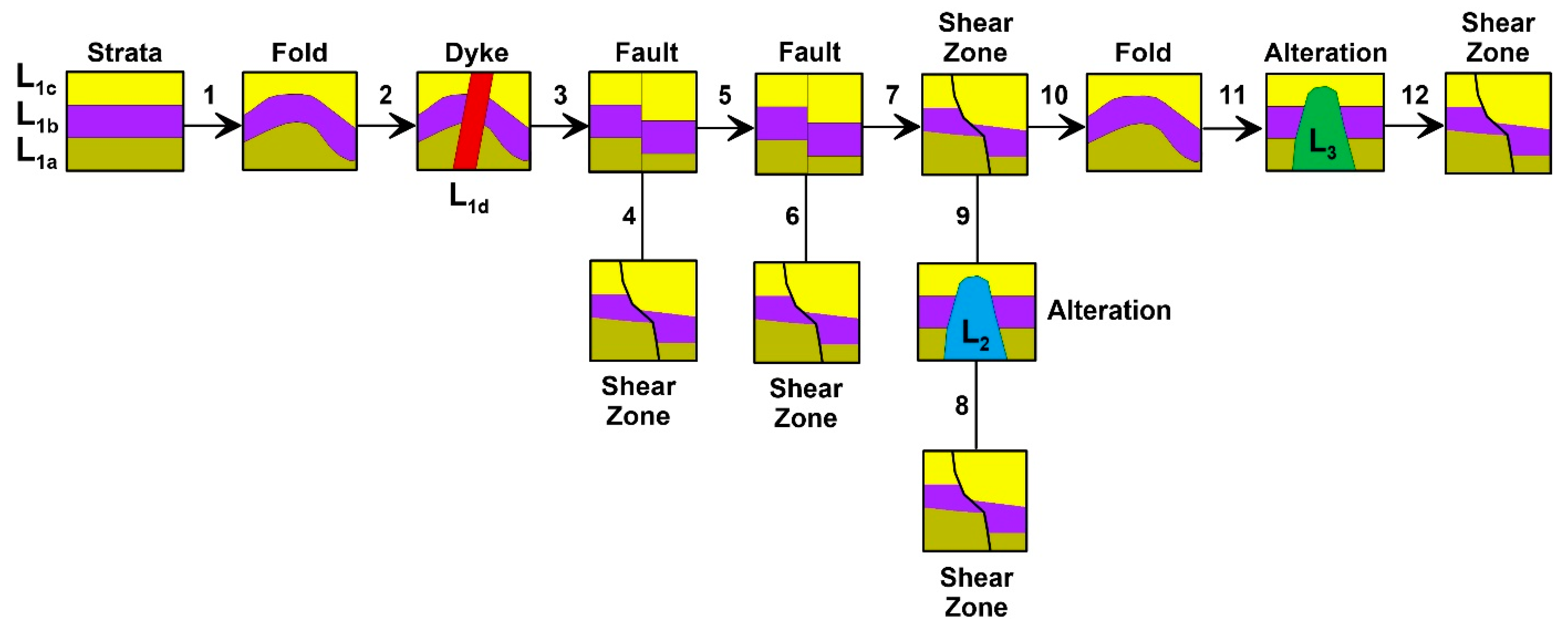
2.2. Simulation of Exploration Procedure

A schematic workflow of a typical exploration procedure is presented in Figure 1a to demonstrate the effect of 3D Earth on geological feature extraction during an exploration program. Minerals comprise macroscopic geological features (L), and a petrophysical system links physical properties (P) to the underlying geological features. The physical properties appear on the Earth’s surface as geophysical signals (S) observed in the form of magnetic and electrical potential fields. The imaging system aims to recover approximated physical property models (P*) from observed signals to be interpreted in the feature extraction system for retrieving an approximation of the latent lithotypes (Li*). Physical properties and lithotypes marked with an asterisk (Pj* and Li*) indicate that they are approximations of the underlying physical properties and lithological variations.
The proposed feature extraction procedure enables us to simulate the interpretation system for quantitative geological feature extraction. We simulated an exploration system to test our source separation methodology. Figure 1b represents a simulation of the exploration process that is used throughout this study. The linear mixing system (petrophysical system in Equation (1) creates physical properties (Pj) from linear mixtures of the hidden lithological factors (Li). The simulation of the geophysical system consists of a well-posed set of equations that calculates the geophysical responses (Sc) of the 3D physical property distributions on the Earth surface (forward modeling).
Sc = f(Pj)
where f represents a forward problem operator that simulates the target geophysical responses (signals), and c = 1, 2, 3, …, p denotes the number of p data points. Through this, we simulated the synthetic field data (Sd) to be fed into the imaging system with an added non-Gaussian geophysical noise (SNoise).
Sd = Sc + SNoise
where d = c.
We inserted two sources of noise: geological and geophysical non-Gaussian noises. The added noises helped us to compare the sensitivity of different feature extraction methods to the unknown sources of outliers. We used a finite element method on the three physical property models to calculate their apparent resistivity, chargeability, and total magnetic field responses [29,30,31]. In the case of the DC/IP forward problem, the IP chargeability model is considered as a small perturbation of the reference electrical conductivity model [30,32]. Normalized chargeability (0 ≤ m ≤ 1) tends to decrease the reference conductivity ( σ D C ) in the modeled IP phenomenon and produces a perturbed subsurface conductivity ( σ I P ) in the function of [32] as follows:
σ I P = ( 1 m ) σ D C
The program calculates the forward potential responses of two conductivity models ( σ D C & σ I P ) separately. The forward modeling σ D C gives the apparent conductivity values ( σ a ), and the modeled potentials ( ϕ ) are used to calculate the apparent chargeabilities based on [32].
m a = [ ϕ ( σ I P ) ϕ ( σ D C ) ] / ϕ ( σ D C )
The imaging system approximates the physical properties (Pj*) through inverse modeling as follows:
P j * = f 1 ( S d )
where f −1 is the inverse problem operator. The recovered physical properties are then used to reconstruct the hidden geological factors (Li*) through the higher-order statistical unmixing process (Equation (2)).
In this study, we explore the effect of the smoothness and sharpness of the imaging system on the output of the feature extraction system. This gives us a valuable view of the way the sharpness of the imaging system could influence the recovered geological features and provides means to predict how much information is essentially extractable from geophysical imaging, i.e., to determine which parts of the spatial domain of the original geology are vulnerable to the information loss due to the geophysical imaging.
We explore the two endpoints of the imaging scenarios (sharp versus smooth) in DC/IP and magnetic inversions. We used a blocky inversion method for the inversion of electrical resistivity and chargeability data [31,33,34] and an iterative reweighting inversion [35,36] for inverse modeling of the magnetic susceptibility data. In each iteration of DC/IP inversion, an incomplete Gauss-Newton least-squares optimization tries to reduce the gap between measured and calculated properties ( σ a and m a ) by modifying the σ D C and σ I P values. When the calculation reaches its threshold, the modeled resistivities and chargeabilities are determined by ρ = 1 / σ D C and m = [ 1 ( σ I P / σ D C ) ] , respectively.
The blocky inversion algorithm [34], which uses an extension of l2-norm and l1-norm inversions, incorporates two cut-off factors in the DC/IP inversion—a data constraint cut-off factor ( 0 < k 1 < 1 ), and a model constraint cut-off factor ( 0 < k 2 < 1 ). Large enough cut-off factors result in smooth physical property models equivalent to l2-norm results. The iterative reweighting magnetic inversion takes the first iteration susceptibility and uses it as an iterative reweighting constraint when running a new inversion. This process is iterated until a satisfactory model is achieved [35,36]. Reweighting magnetic inversion tends to recover sharp magnetic variations, and its results are equivalent to the robust or blocky inversion in the DC/IP inversion [33,34].

2.3. Independent Component Analysis (ICA)

Traditional visualization techniques incorporating conventional gridding, slicing, and clipping methods cannot identify subtle structures inside the high-dimensional geophysical images. In the presence of statistical correlation and independence, multivariate tools are necessary to recover the hidden patterns inside multiple interdependent geophysical images. Statistical measures provide collective clues about the behaviors of multivariate spaces. Instead of treating every geophysical image separately, one can extract the underlying features by making few general assumptions about the multivariate statistical measures. The mixing process has three statistical characteristics [37] that need to be considered to reconstruct an integrated geological model from physical properties. Firstly, the source geological features are statistically uncorrelated and independent, while the physical properties are correlated and interdependent due to the linear mixing process. Secondly, the mixing process increases the normality or Gaussianity of the images, i.e., the observed (or modeled) physical property images are more Gaussian than the underlying lithological distributions. This results from the central limit theorem (CLT) in probability theory that says the distribution of a sum of independent random variables tends toward a Gaussian distribution. Later, we used this principle to maximize the non-Gaussianity of physical properties using kurtosis maximization as a criterion for estimating hidden geological features. Thirdly, the spatial complexities of the physical property images are equal to or greater than that of the least complex geological feature distribution. We later used this general principle to maximize the non-Gaussianity of physical properties using negentropy maximization as a criterion for estimating hidden geological features.
One crucial statistical measure is correlation. It is very common for two geophysical properties imaged by two different methods to be correlated. For example, if a perfect linear relationship exists between a magnetic susceptibility image and an electrical resistivity image, the amount of information that the first image provides is the same as the second one. Therefore, one can transfer the bivariate data to a univariate form without losing any valuable information. This transformation is called dimensionality reduction that is the basis of PCA algorithms [37,38]. PCA is the standard method for unmixing the correlated images. PCA produces linearly uncorrelated images, and this approach is usually called whitening because this is the property of the white noise. PCA algorithms utilize the maximization of second-order statistical measure (variance) for image separation. However, when there is a nonlinear form of correlation (dependency) between images, PCA will not work, and one needs to find another way to unmix interdependent images [38,39].
On the other hand, ICA separates mixed images into nonlinearly uncorrelated images through the maximization of multivariate non-Gaussianity. The one-dimensional ICA analogy is well known as a classical cocktail party problem [40], where people are talking independently together. By incorporating two or more receivers, it is impossible to detect each conversation independently. For example, the human auditory system, with two receivers, hears a mixture of signals in a cocktail party and can differentiate the source to a certain degree. However, by installing several microphones and maximizing the non-Gaussianity of received signals, we will be able to separate more voices. The same analogy is applied to neuroscience, where the spatiotemporal ICA problem in medical imaging is compared to a neurological cocktail party problem by Von der Malsburg and Schneider [41] and Brown [42]. Perhaps, a 3D equivalent to this 1D blind source separation could be called a geophysical cocktail party problem, where geophysicists try to detect the rocks’ hidden information inside mixtures of different physical property images.
Traditionally, ICA algorithms seek to maximize higher-order measures such as skewness (third-order measure) and kurtosis (fourth-order measure). Another approach is the application of information theory principles for the maximization of non-Gaussianity. This study proposes a 3D model-based Fast-ICA algorithm based on the study by Hyvärinen et al. [39], which utilizes two different non-Gaussianity maximization approaches—kurtosis maximization and negentropy maximization.
Fast-ICA algorithm starts with two preprocessing steps: first, removing the mean of input physical properties and then whitening by PCA giving their variance unit value. PCA looks for a weight matrix D so that a maximal variance of the principal components of the central physical properties (YPC) are confirmed as follows:
Y P C = D T P
Optimization of PCA criterion is possible by eigenvalue decomposition [39]. The next step in the Fast-ICA algorithm is to increase the non-Gaussianity of the principal components. The problem is to find a rotation matrix R that during the multiplication with principal components produces the least Gaussian outputs (L*) that are approximations of the original geological features.
L * = R T Y P C
One way to calculate the rotation matrix R is to use kurtosis as a measure of non-Gaussianity as follows:
k u r t ( L * ) = E ( ( R T Y P C ) 4 ) 3 { E ( ( R T Y P C ) 2 ) } 2
where E(.) denotes the expected value. Kurtosis provides a measure of how Gaussian (kurt = 0), super-Gaussian (kurt > 0) or sub-Gaussian (kurt < 0) the probability density functions of the physical properties are. Therefore, the highest non-Gaussianity of L* is equivalent to the maximum or minimum excess kurtosis of its distribution. In this study, we used a fixed-point iteration scheme of Hyvärinen and Oja [15], where each point in a converging sequence is a function of the previous one. Fast-ICA has a fast quadratic or cubic convergence and requires slight memory space [16]. However, kurtosis is not a robust measure of non-Gaussianity in the presence of noise. Kurtosis is an approximated measure of the fourth central moment of the probability density function of data, and to calculate it accurately, we need to have an infinite number of physical property values. This makes kurtosis very sensitive to outliers, i.e., a single erroneous outlier value in the distribution’s tails makes kurtosis extremely large. Therefore, using kurtosis is well justified when the independent components (geological features) are sub-Gaussian, and there are no outliers (geological noises or other artifacts on physical property images).
Therefore, we needed to assess non-Gaussianity in a different way that can handle the fluctuations of outliers. Alternatively, the maximization of negentropy is a robust technique for obtaining the rotation matrix R during the Fast-ICA procedure. Negentropy (normalized differential entropy) of a signal is the difference between the entropy H (L*) of that signal and the entropy H (Lgauss) of a Gaussian random vector of the same covariance matrix as L*. Negentropy of the L*, therefore, is
n e g ( L * ) = H ( L g a u s s ) H ( L * )
Negentropy is always non-negative and is zero when the signal has Gaussian distribution. In other words, the more random (unpredictable and unstructured) the variable is, the larger its entropy. We approximate the negentropy through the following nonpolynomial method:
n e g ( L * ) c [ E { G ( L * ) } E { G ( L s t d ) } ] 2
where c is an irrelevant constant, and Lstd is a standardized Gaussian variable (Lgauss of zero mean and unit variance). G is a non-quadratic exponential function that can handle the outliers efficiently [16].
G ( L * ) = e ( L * 2 2 )
To find the rotation matrix R, the objective negentropy is maximized using a fixed-point algorithm [39].

3. Results

3.1. Simulation of Petrophysical System

The purpose of this study is to show numerically how the overlapped geological features seen in the form of physical properties appear as geophysical signals on the Earth’s surface, and how geological/geophysical noises and inversion artifacts influence the process of feature extraction. Therefore, we were not concerned with the construction of any specifically existing geological model from mineral exploration literature. We used a range of physical property values (minimum and maximum) based on a reasonable average of electrical resistivities, IP chargeabilities, and magnetic susceptibilities of disseminated sulfide deposits [2] that provided us enough spatial complexity to test our feature extraction methodology.
The basic lithology model was constructed from an original layered Earth model passed through several faulting, folding, dyke intrusion, shear deformation, and alteration overprints (Figure 2 and Figure 3). The final 3D lithology model (stage 12 in Figure 3) included a set of background rock units (L1a, L1b, L1c, L1d) and two stages of hydrothermal alteration in the form of plug-shaped alteration overprints (L2 and L3). Figure 4 represents the last episode of the geological history stored as six independent lithotypes to be used later in this study.
The linear overlap of the four rock units and the two alteration events comprised three physical property distributions: electrical resistivity, induced polarization chargeability, and magnetic susceptibility. A mixing system was built to simulate a disseminated sulfide deposit, where background rock units are intruded by two distinct disseminated sulfide-rich alteration events with the following mixing matrix form (Equation (1)).
L 1 L 2 L 3 A = [ 0.9 0.05 0.05 0.5 0.2 0.75 0.45 0.25 0.3 ] ρ = 0.90 L 1 + 0.05 L 2 + 0.05 L 3 m = 0.05 L 1 + 0.20 L 2 + 0.75 L 3 χ = 0.45 L 1 + 0.25 L 2 + 0.30 L 3
Equation (14) means that 90 percent of the first physical property (P1 = ρ; electric resistivity) is derived from the background rocks (L1a, L1b, L1c, L1d), 5 percent from the alteration L2, and 5 percent from the alteration L3. The second physical property is induced polarization chargeability (P2 = m), which is least sensitive to the background geology (5 percent), and 20 percent and 75 percent of it result from the two alteration events (L2 and L3). Note that 75 percent of chargeability comes from the alteration L3, which means L3 bears the largest amount of disseminated sulfides. The magnetic susceptibility (P3 = χ) represents 45 percent of the background geology, 25 percent the alteration L2 and 30 percent the alteration L3. The resulting mixtures were then scaled from zero to a reasonable maximum; set to 500 Ohm-m, 100 mV/V, and 0.1 SI for resistivities, chargeabilities, and susceptibilities.
Figure 5 shows the calculated physical property models. An additional non-Gaussian noise accompanies the mixing process to simulate a realistic geological environment where the lithologies are heterogeneous. We used a Pearson random system to create this geological noise in the form of a 3D matrix with unit standard deviation and skewness equal to 1 for resistivity and chargeability models and skewness equal to −1 for the susceptibility model. The kurtosis of the geological noise was set to 5 for the resistivity model and 4 for the chargeability and susceptibility models.
The histograms of the original litho-codes and the simulated physical properties are shown in Figure 6. As can be seen, the histograms of physical properties (Figure 6d–f) show the multimodal nature of the physical properties due to the mixing process. However, the added non-Gaussian geological noise smooths some smaller patterns related to the overlaps of the rock’s units with two alteration episodes (Figure 6g–i). We also predict that the passage of lithological information from the geophysical system and then the imaging system will significantly reduce this multimodality to bimodality or even unimodality. This information loss is one of the major limitations of 3D geophysical imaging that we aim to tackle in this study quantitatively.
This study used a three-component geological model and a three-component physical property model to avoid too many drawn-out interpretations. However, in practice, we can use any number of geological features and physical properties, including seismic velocities and bulk densities, for 3D seismic tomography and gravity modeling. Nevertheless, to avoid inconsistency, we kept the number of geological features equal to or less than the physical properties (nm).

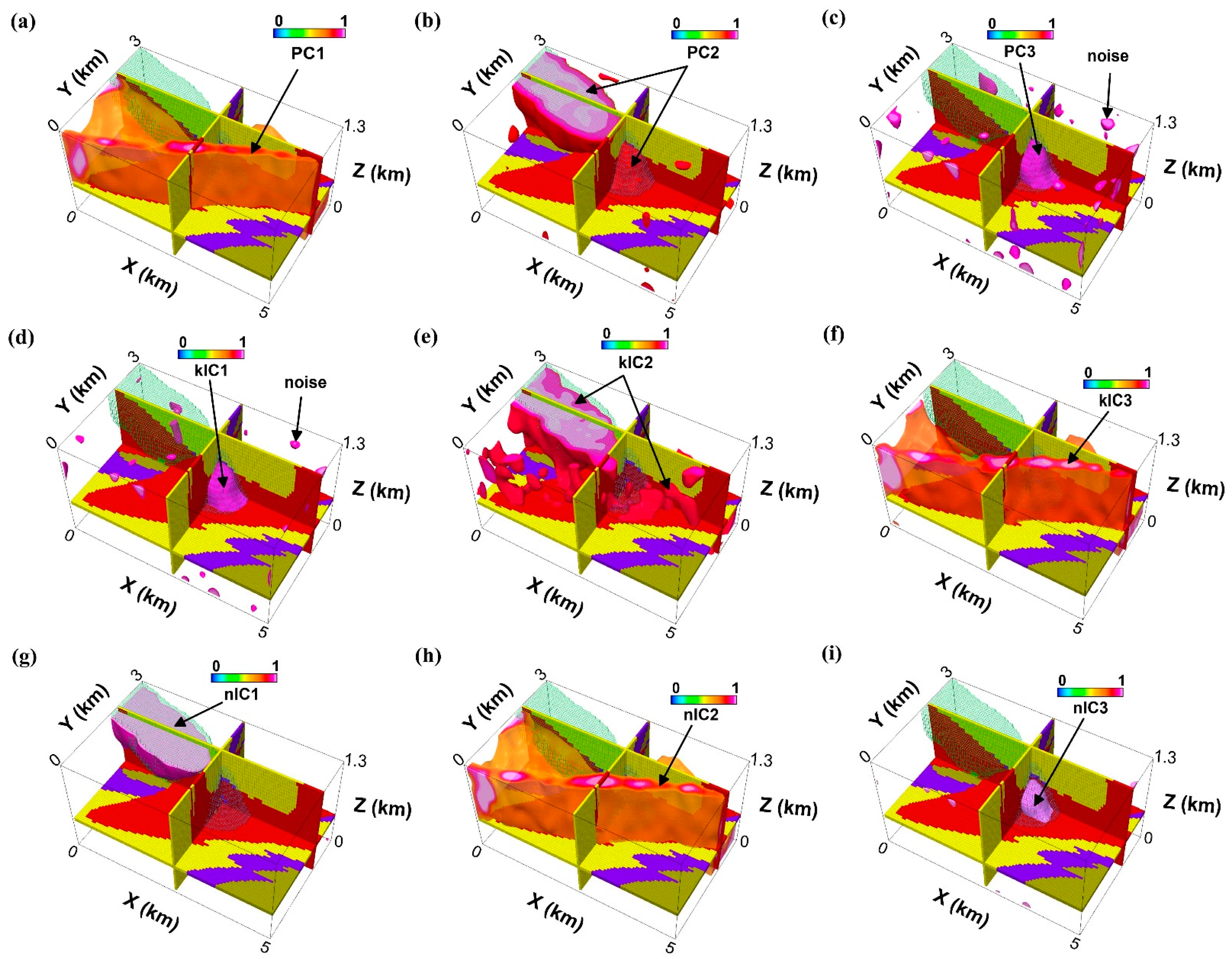
3.2. Petrophysical Feature Extraction

We evaluated different source separation algorithms to see which method was more stable in the recovery of lithological factors in the presence of the non-Gaussian noise on the mixed physical properties. The objective is to recover the two separate alteration events from the background lithology, supposing that the imaging system has zero influence on the source separation, equivalent to a situation where geophysical inversion accurately recovers physical properties. This strategy will help us to compare the exact results to the more realistic scenario of an approximate inverse solution to understand the effect of the geophysical and imaging systems on the source separation process.
Running PCA to separate images did not yield efficient separate geological features, and another form of mixture remained on the principal components (Figure 7a–c). Even if the recovered principal components of the physical properties are uncorrelated, knowing the values of one image still provides information about the other image. However, the first and third principal components (PC1 and PC3 in Figure 7a,c) successfully represent the background geology (L1) and the first alteration event (L2), but the third alteration event (L3) is still mixed with the second alteration event in the second principal component (PC2 in Figure 7b).
Fast-ICA by kurtosis maximization could neither tolerate the mixing system’s added geological noise, resulting in few overlapped features in the separated outputs (Figure 7d–f). However, Fast-ICA by negentropy maximization recovered the underlying geological features almost perfectly. As can be seen (Figure 7g–i), negentropy maximization can efficiently handle the added non-Gaussian background geological noise separating the main geological features.

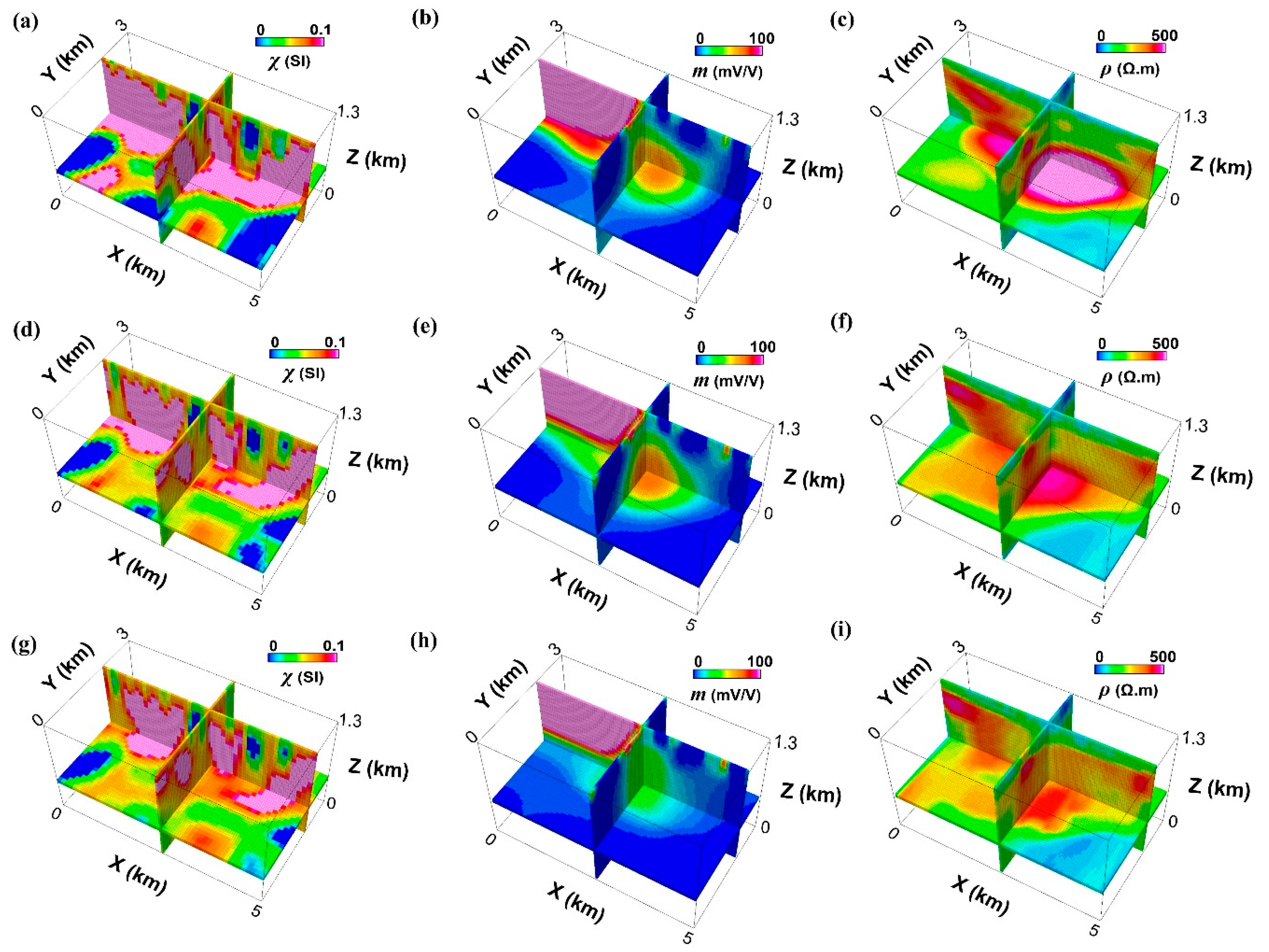
3.3. Simulation of the Geophysical System (Forward Modeling)

We calculated the geophysical responses of the mixed physical properties to explore how the interdependent physical properties appear as geophysical signals on the surface of the Earth. This is a more realistic assumption because most geophysical data are gathered on the surface and are apparent indicators of 3D underground physical property distributions.
The DC/IP apparent physical properties were simulated over the mixed physical properties with pole–dipole electrode configurations, dipolar spacing of 100 m, and dipolar separations up to 12 times in X and Y directions. The model mesh consists of 151 cells in the X direction, 111 cells in the Y direction, and 38 cells in the Z direction with two nodes between the adjacent electrodes, which simulates the forward electrical potentials of 51 electrodes in the X direction and 31 electrodes in the Y direction. Therefore, the total number of electrodes is 1581, over a 3D discretized volume with 636918 rectangular cells.
The same magnetic station intervals were applied for magnetic forward modeling, i.e., 100 m spacing between observation points in both the X and Y directions. The magnetic field over the 3D volume is set to 29,639 nT with inclination and declination of 21° and 1°, respectively. We assumed that there is no remanent magnetization contributing to the surface observations and that demagnetization of rocks is negligible.
We calculated the forward responses over the 3D rectangularly gridded physical properties using forward modeling algorithms introduced in Li and Oldenburg [29,30]. Figure 8 shows the forward responses of the magnetic and DC/IP models in the form of total magnetic field intensities (after reduction to magnetic pole), apparent resistivities, and apparent chargeabilities.

3.4. Imaging System (Inverse Modeling)

One of the main objectives of this study was exploring the sensitivity of feature extraction to the tuning of the imaging system. Through inverse modeling (imaging system), we sought to recover the physical properties with different adjustments of the inversion parameters. Finally, we unmixed the recovered physical properties (in the unmixing system) to approximate the underlying lithological factors. We evaluated how the imaging system (inversion) can distort the unmixing process during the inference of the lithological factors. Though the mixing system behaves linearly, the Earth forward response (geophysical system in Figure 1), and the reconstruction of physical properties (imaging system in Figure 1) add unwanted artifacts to the inverted physical property images, specifically when we executed unconstrained 3D inversions due to the lack of prior petrophysical information.
A set of underlying inversion parameters were set to recover sharp images of the physical properties. The blocky DC/IP inversion was controlled by different cut-off factors to examine the effect of inversion artifacts on the outputs of the feature extraction algorithm. Achieving a value too close to the l2-norm criteria (larger cut-off factors) increased the misfit error, and closer to l1-norm (smaller cut-off factors) produced too sharp boundaries that distorted the 3D continuity of the models. We used three representative DC/IP inversion episodes with the following parameters: the first DC/IP inversion with a data constraint cut-off factor k1 = 1 and a model constraint cut-off factor k2 = 1 (smoothest physical properties); the second DC/IP inversion with k1 = 0.1 and k2 = 0.05 (sharper physical properties); the third DC/IP inversion with k1 = 0.01 and k2 = 0.005 (sharpest physical properties).
Three episodes (iterations) of the iterative reweighing magnetic inversion were also used to produce three smooth-to-sharp representative susceptibility models. The recovered physical properties (Figure 9) exhibit valuable information about the underlying features, but some of the key background geological features are missed due to the imaging process. The first imaging scenario (smoothest) was tuned to recover approximations of physical properties (ρ, m, and χ), where the sharpness of images was enough to capture an overall view of the underlying geological features (Figure 9a–c). However, increasing the depth of investigation in the smooth inversions deforms the shape of the first alteration event that is the deepest one (L2 in Figure 4f). Increasing the level of sharpness in Figure 9d–f focuses more on the hidden geological features. However, the two alteration events are still attached. The sharpest images are presented in Figure 9g–i, where the lithological background is much more visible in the resistivity and susceptibility images (Figure 9g–i), and two alteration events are more confined in the modeled chargeability image (Figure 9h).

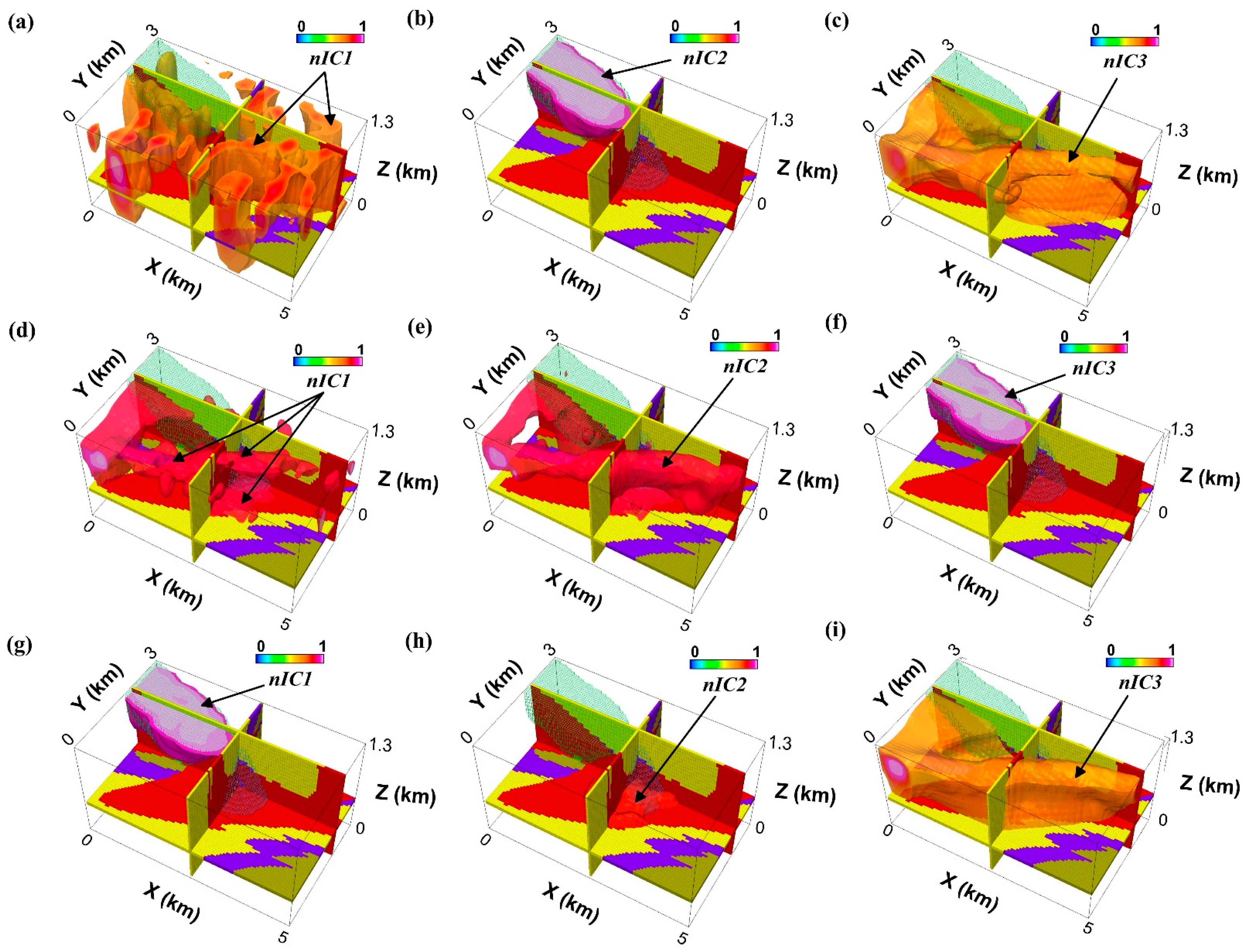
3.5. Post-Inversion Feature Extraction

We evaluated the effect of imaging systems (inverse modeling) on the performance of feature extraction. We explored different inversion procedures to investigate how artifacts from the imaging system leak into the estimated physical properties and then distort the performance of geological feature extraction. We do not show the results of the PCA and ICA by kurtosis maximization because we already showed that they were not as efficient as the negentropy maximization algorithm. The major difference between pre-inversion (petrophysical) and post-inversion feature extraction is that the depth estimation in the post-inversion physical properties leads to distorted physical property images and erroneous reconstructed geological features.
The post-inversion feature extraction results are shown in Figure 10 for the three inversion scenarios. The independent components of the smoothest physical properties (Figure 10a–c) keep some of the latent features mixed, which is understandable due to the smoothness artifacts leaked into the imaging and feature extraction systems. The third alteration event is clearly extracted in the second independent component (nIC2), but the background geology and the first alteration event were mixed in the other independent components (nIC1 and nIC3).
Running a sharper inversion helped to increase the contrast of the models. However, a certain amount of information is still lost during the imaging process. Again, the second alteration event is clearly extracted in the third independent component (nIC3 in Figure 10f), and the background geology is extracted in the second independent component (nIC2 in Figure 10e). However, the first independent component (nIC1 in Figure 10d) could not separate the first alteration event from background geology.
The separation of the sharpest physical property images results in the most accurate geological features (Figure 10g–i). Both alteration events are successfully extracted as distinct independent components (nIC1 and nIC2 in Figure 10g,h). The third independent component also extracts a more accurate image of the latent background geology (nIC3 in Figure 10i).

4. Discussion

Cross plots of the physical properties and extracted independent components were compared to the initial geological features to evaluate the feature extraction performance for both pre-inversion petrophysical and post-inversion feature extractions (Figure 11). As shown in Figure 11a,b, the original petrophysical system produces overlapped expressions of the latent geological features, where the background geological features are overprinted with the two alteration events. The inverted physical properties from the imaging system show a distorted background geological pattern, where the intruded dyke (L1d) is visually separable from a mixture of older strata (L1a, L1b, and L1c).
The overprints of alteration events were also imaged as overlapped patterns occupying the same space. Without any prior petrophysical information, it is very hard to differentiate two alteration events from each other and the background geology. The pre-inversion petrophysical feature extraction extracted three independent components that are representative of three underlying geological features (Figure 11e). The background geological dyke and the two alterations are clearly separated into three separated regions. The post-inversion extracted features are also separated into three distinct groups, though there are still few overlaps in some places (Figure 11f).
Though the negentropy maximization captures the first plug-shaped alteration event (deep feature), the recovered geometrical shape of that is not accurate, which is a side effect of the geophysical inversion artifacts disturbing the feature extraction process. Specifically, the non-uniqueness of magnetic inversion results in erroneous susceptibilities at deeper levels that masked the first alteration event on the susceptibility image.
To reduce the non-uniqueness of the magnetic inversion, we suggest performing a cooperative inversion that utilizes DC/IP inversion to constrain the magnetic inversion. The similarity between two physical property distributions (resistivity and susceptibility in this case) allows us to run a cooperative inversion. In this case, 90 percent of the background geology is detectable in the original resistivity image, in contrast to the 45 percent of it that is detectable in the original susceptibility image, making it possible to use the recovered resistivity model to constrain the magnetic inversion cooperatively. This approach probably increases the accuracy of the recovered susceptibility image; however, the potential field nature of the DC/IP inversion also causes a certain number of geological features to go missing during the imaging process.
One way to increase the accuracy of the physical property estimation is to add other techniques such as seismic and electromagnetic imaging in a multistage and iterative cooperative modeling procedure, where information from each physical property inversion is used to constrain the other inversions as far as all physical property models converge into a satisfactory result on the last iteration. The other way is to use borehole constraints to reduce the non-uniqueness of the physical property models through constrained inversion.

5. Conclusions

This study applied kurtosis and negentropy maximization in an independent component analysis framework for geological feature extraction from multiple 3D geophysical images with latent geological features. We presented a 3D post-inversion method for geological feature extraction from multiple geophysical images, where negentropy of multiple physical properties are maximized as a criterion of Fast-ICA for extraction of latent geological features from 3D geophysical images. The methodology was tested through simulation of a typical exploration procedure that provided a way to transform 3D geological features to overlapped physical property models linearly. The simulation also involved the calculation of geophysical responses of the 3D physical properties on the Earth’s surface. We used the resulting synthetic geophysical signals to recover the 3D physical properties and the hidden geological features.
We explored efficiencies of different source separation methods and showed that the negentropy maximization is superior to the variance and kurtosis maximization in tolerating the added non-Gaussian geological and geophysical noises. We also explored the effect of the inversion artifacts on the performance of Fast-ICA through negentropy maximization. The results showed that the smooth inversions result in spurious physical property artifacts permeated to the ICA, destabilizing the feature extraction system, producing another form of mixed features in the output components. However, increasing the sharpness of the inversions produced sharper physical property images, enhanced the feature extraction performance, and successfully recovered more geological features.
We used a three-feature geological system and a three-component physical property model in this study. However, in practice, we can use any number of geological features and physical properties. The simulation of the petrophysical system allowed us to study the effect of spatially coexisting patterns inside multidimensional physical properties. Interpretation of these types of complicated and mixed geological systems is a challenge to post-inversion qualitative geophysical interpretations.
The proposed feature extraction method is a powerful tool for post-inversion semi-automatic interpretations and needs no prior geological or petrophysical information for geological feature extraction. The methodology is also applicable to many other exploration scenarios where geophysicists are interested to understand the whole process of geophysical interpretation from data gathering to inversion and post-inversion interpretations.

Author Contributions

Conceptualization, B.A. and L.-Z.C.; methodology, B.A.; software, B.A.; validation, B.A. and L.-Z.C.; formal analysis, B.A.; investigation, B.A.; resources, B.A.; data curation, B.A.; writing—original draft preparation, B.A.; writing—review and editing, B.A. and L.-Z.C.; visualization, B.A.; supervision, L.-Z.C.; project administration, L.-Z.C.; funding acquisition, L.-Z.C. All authors have read and agreed to the published version of the manuscript.

Funding

This research was funded by Natural Sciences and Engineering Research Council of Canada (NSERC), Fonds de recherche, Nature et technologies du Québec (FRQNT), and ministère de l’Énergie et des Ressources naturelles du Québec (MERNQ).

Conflicts of Interest

The authors declare no conflict of interest.

References

  1. Lelièvre, P.G.; Farquharson, C.G. Integrated Imaging for Mineral Exploration. In Integrated Imaging of the Earth: Theory and Applications; Geophysical Monograph 218; Moorkamp, M., Ed.; Wiley Online Library: Hoboken, NJ, USA, 2016; pp. 61–95. [Google Scholar] [CrossRef]
  2. Dentith, M.; Mudge, S.T. Geophysics for the Mineral Exploration Geoscientist; Cambridge University Press: Cambridge, UK, 2014. [Google Scholar] [CrossRef] [Green Version]
  3. Fullagar, P.K.; Hughes, N.A.; Pain, J. Drilling constrained 3D gravity inversion. Explor. Geophys. 2000, 31, 17–23. [Google Scholar] [CrossRef]
  4. Wisen, R.; Christiansen, A.V. Laterally and mutually constrained inversion of surface wave seismic data and resistivity data. J. Environ. Eng. Geophys. 2005, 10, 251–262. [Google Scholar] [CrossRef] [Green Version]
  5. Lelièvre, P.G. Integrating Geologic and Geophysical Data through Advanced Constrained Inversions. Ph.D. Thesis, The University of British Columbia, Vancouver, BC, Canada, 2009. Available online: http://hdl.handle.net/2429/6661 (accessed on 29 July 2021).
  6. Lelièvre, P.G.; Oldenburg, D.W.; Williams, N.C. Integrating geological and geophysical data through advanced constrained inversions. Explor. Geophys. 2009, 40, 334–341. [Google Scholar] [CrossRef]
  7. Lines, L.R.; Schultz, A.K.; Treitel, S. Cooperative inversion of geophysical data. Geophysics 1988, 53, 8–20. [Google Scholar] [CrossRef]
  8. Paasche, H.; Tronicke, J. Cooperative inversion of 2D geophysical data sets: A zonal approach based on fuzzy c-means cluster analysis. Geophysics 2007, 72, A35–A39. [Google Scholar] [CrossRef]
  9. Haber, E.; Oldenburg, D. Joint inversion: A structural approach. Inverse Probl. 1997, 13, 63–77. [Google Scholar] [CrossRef]
  10. Doetsch, J.; Linde, N.; Coscia, I.; Greenhalgh, S.; Green, A. Zonation for 3D aquifer characterization based on joint inversion of multimethod crosshole geophysical data. Geophysics 2010, 75, G53–G64. [Google Scholar] [CrossRef]
  11. Chen, J.; Hoversten, G.M. Joint inversion of marine seismic AVA and CSEM data using statistical rock-physics models and Markov random fields. Geophysics 2012, 77, R65. [Google Scholar] [CrossRef]
  12. Gallardo, L.A.; Fontes, S.L.; Meju, M.A.; Buonora, M.P.; de Lugao, P. Robust geophysical integration through structure-coupled joint inversion and multispectral fusion of seismic reflection, magnetotelluric, magnetic and gravity images: Example from Santos Basin, offshore Brazil. Geophysics 2012, 77, B237–B251. [Google Scholar] [CrossRef]
  13. Haber, E.; Gazit, M.H. Model fusion and joint inversion. Surv. Geophys. 2013, 34, 675–695. [Google Scholar] [CrossRef]
  14. Comon, P. Independent component analysis: A new concept. Signal Process. 1994, 36, 287–314. [Google Scholar] [CrossRef]
  15. Hyvärinen, A.; Oja, E. A fast fixed-point algorithm for ICA. Neural Comput. 1997, 9, 1483–1492. [Google Scholar] [CrossRef]
  16. Hyvärinen, A.; Karhunen, J.; Oja, E. Independent component analysis. In Adaptive and Learning Systems for Signal Processing, Communications, and Control; Haykin, S., Ed.; John Wiley & Sons, Inc.: Hoboken, NJ, USA, 2001. [Google Scholar] [CrossRef]
  17. Hyvärinen, A. Independent component analysis: Recent advances. Phil. Trans. R. Soc. A 2013, 371, 1984. [Google Scholar] [CrossRef] [PubMed] [Green Version]
  18. Bayliss, J.D.; Gualtieri, J.A.; Cromp, R.F. Analyzing hyperspectral data with independent component analysis. In Proceedings of the 26th AIPR Workshop: Exploiting New Image Sources and Sensors, Washington, DC, USA, 15–17 October 1998; International Society for Optics and Photonics: Washington, DC, USA, 1998; pp. 133–143. [Google Scholar]
  19. Amato, U.; Antoniadis, A.; Cuomo, V.; Cutillo, L.; Franzese, M.; Murino, L.; Serio, C. Statistical cloud detection from SEVIRI multispectral images. Remote Sens. Environ. 2008, 112, 750–766. Available online: https://spie.org/Publications/Proceedings/Paper/10.1117/12.300050 (accessed on 29 July 2021). [CrossRef]
  20. Barnie, T.; Oppenheimer, C. Extracting high temperature event radiance from satellite images and correcting for saturation using Independent Component Analysis. Remote Sens. Environ. 2015, 158, 56–68. [Google Scholar] [CrossRef] [Green Version]
  21. Liu, B.; Dai, W.; Peng, W.; Meng, X. Spatiotemporal analysis of GPS time series in vertical direction using independent component analysis. Earth Planets Space 2015, 67, 189. [Google Scholar] [CrossRef] [Green Version]
  22. Choudrey, R.; Roberts, S. Variational mixture of Bayesian independent component analysers. Neural Comput. 2002, 15, 213–252. [Google Scholar] [CrossRef]
  23. Beckmann, C.F.; Smith, S.M. Probabilistic independent component analysis for functional magnetic resonance imaging. IEEE Trans. Med. Imaging 2004, 23, 137–152. [Google Scholar] [CrossRef]
  24. Griffanti, L.; Salimi-Khorshidi, G.; Beckmann, C.F.; Auerbach, E.J.; Douaud, G.; Sexton, C.E.; Zsoldos, E.; Ebmeier, K.P.; Filippini, N.; Mackay, C.E. ICA-based artefact removal and accelerated fMRI acquisition for improved resting state network imaging. NeuroImage 2014, 95, 232–247. [Google Scholar] [CrossRef]
  25. Jenssen, R.; Eltoft, T. Independent component analysis for texture segmentation. Pattern Recognit. 2003, 36, 2301–2315. [Google Scholar] [CrossRef]
  26. Zou, W.; Li, Y.; Lo, K.C.; Chi, Z. Improvement of image classification with Wavelet and Independent Component Analysis (ICA) based on Structured Neural Networks. In Proceedings of the IEEE International Conference on Neural Networks 2006, Vancouver, BC, Canada, 24–29 July 2006; pp. 3949–3954. [Google Scholar] [CrossRef]
  27. Van der Baan, M. PP/PS Wavefield separation by independent component analysis. Geophys. J. Int. 2006, 166, 339–348. [Google Scholar] [CrossRef] [Green Version]
  28. Honório, B.C.Z.; Sanchetta, A.C.; Leite, E.P.; Vidal, A.C. Independent component spectral analysis. Interpretation 2014, 2, 1. [Google Scholar] [CrossRef]
  29. Li, Y.; Oldenburg, D.W. 3D inversion of magnetic data. Geophysics 1997, 61, 394–408. [Google Scholar] [CrossRef]
  30. Li, Y.; Oldenburg, D.W. 3D inversion of induced polarization data. Geophysics 2000, 65, 1931–1945. [Google Scholar] [CrossRef] [Green Version]
  31. Tutorial: 2D and 3D Electrical Imaging Surveys: Geotomo Software. Available online: http://www.geotomosoft.com/downloads.php (accessed on 29 July 2021).
  32. Oldenburg, D.W.; Li, Y. Inversion of induced polarization data. Geophysics 1994, 59, 1327–1341. [Google Scholar] [CrossRef]
  33. Claerbout, J.F.; Muir, F. Robust modeling with erratic data. Geophysics 1973, 38, 826–844. [Google Scholar] [CrossRef]
  34. Loke, M.H.; Acworth, I.; Dahlin, T. A comparison of smooth and blocky inversion methods in 2D electrical imaging surveys. Explor. Geophys. 2003, 34, 182–187. [Google Scholar] [CrossRef]
  35. Portniaguine, O.; Zhdanov, M.S. 3-D magnetic inversion with data compression and image focusing. Geophysics 2002, 67, 1532–1541. [Google Scholar] [CrossRef] [Green Version]
  36. Sharpening using Iterative Reweighting Inversion: Oasis Montaj Best Practice Guide. Available online: http://updates.geosoft.com/downloads/files/how-to-guides/Best-Practice-Guide_Sharpening_using_IRI.pdf (accessed on 29 July 2021).
  37. Hyvärinen, A.; Oja, E. Independent component analysis: Algorithms and applications. Neural Netw. 2000, 13, 411–430. [Google Scholar] [CrossRef] [Green Version]
  38. Trauth, M.H. MATLAB Recipes for Earth Sciences, 4th ed.; Springer: Berlin/Heidelberg, Germany, 2015. [Google Scholar] [CrossRef]
  39. Hyvärinen, A.; Karhunen, J.; Oja, E. Independent Component Analysis; Wiley Interscience Publication: New York, NY, USA, 2002. [Google Scholar] [CrossRef]
  40. Cherry, E.C. Some experiments on the recognition of speech, with one and with two ears. J. Acoust. Soc. Am. 1953, 25, 975–979. [Google Scholar] [CrossRef]
  41. Von der Malsburg, C.; Schneider, W. A neural cocktail-party processor. Biol. Cybern. 1986, 54, 29–40. [Google Scholar] [CrossRef]
  42. Brown, G.D.; Yamada, S.; Sejnowski, T.J. Independent component analysis at the neural cocktail party. Trends Neurosci. 2001, 24, 54–63. [Google Scholar] [CrossRef]
  43. Noddy Structural and Geological Modeling: Reference Manual, TecTask, Encom Technology Pty Ltd. Available online: https://tectonique.net/noddy (accessed on 29 July 2021).
Figure 1. Workflow of geological feature extraction: (a) An exploration system: The synergy of the hidden mixing petrophysical system with the geophysical system creates observed geophysical signals (S) that produce measured physical properties (P). The approximated physical properties (P*) are used in a feature extraction system to recover the hidden geological factors (L). (b) A simulation of the exploration system: Synthetic geophysical signals (Sd) are calculated from the forward responses of the simulated physical properties (Pj) that are linear mixtures of hidden geological features (Li). Multiple inversions calculate the estimated physical properties (Pj*) that are used in the subsequent feature extractions to retrieve an approximation of the latent lithotypes (Li*).
Minerals 11 00959 g001
Figure 2. Workflow of geological model construction. The background geology consisted of a three-layer stratum (L1a, L1b, L1c) intruded by a dyke (L1d). After several faulting and shear deformation, two alteration events (L2 and L3) and further deformations overprinted the host geology. Noddy 3D geological and geophysical modeling package was used to build the geological model [43].
Minerals 11 00959 g002
Figure 3. Construction of geological features. Reference geological model was selected at the end of stage 12 with three major geological features: a background geology (L1a, L1b, L1c, L1d) and two separate alteration overprints overlapped over the background geological features (L2, L3).
Minerals 11 00959 g003
Figure 4. Three independent geological features contribute to the bulk physical properties (a). The background lithology has three components (bd), which is intruded by a dyke (e) and overprinted by two successive alteration events (f).
Minerals 11 00959 g004
Figure 5. The mixing system produces three overlapped physical properties (ρ, m and χ in bd) from simulated geological features (a). Each physical property distribution shows a portion of the whole geological features (bd). The source separation aims to recover the hidden independent features to reconstruct the whole geological model.
Minerals 11 00959 g005
Figure 6. Histograms of simulated physical properties: (ac) Histograms of the original litho-codes used for geological modeling; (df) Histograms of the mixed physical properties (noise-free); (gi) Histograms of the mixed physical properties with added non-Gaussian noise. Multimodal nature of the physical properties is a result of the mixing process. The solid curve indicates the cumulative distribution function.
Minerals 11 00959 g006
Figure 7. Assessment of different source separation methods: (ac) principal components (PC1, PC2, and PC3) from the PCA method; (df) independent components (kIC1, kIC2, and kIC3) from Fast-ICA by kurtosis maximization; (gi) independent components (nIC1, nIC2 and nIC3) from Fast-ICA by negentropy maximization. PCA recreates another set of overlapped images on PC2 and is ineffective in source separation (ac). Fast-ICA by kurtosis maximization produces a set of images (kICs) separated to some extent, but still, some of the features remain mixed in the first and second independent components in the form of outliers, background geology mixed with the second alteration event. Fast-ICA by negentropy maximization produces a set of images (nICs) that are efficiently separated (gi). All principal and independent components were normalized from zero to one for consistency of visualization.
Minerals 11 00959 g007
Figure 8. The geophysical responses (Sd) of the mixed physical properties (Pj): (a) total magnetic field intensities after reduction to magnetic pole; (b) apparent resistivities; (c) apparent chargeabilities. DC/IP responses are presented on two NS and EW pseudo-sections as well as a horizontal slice corresponding to the dipolar separation of n = 9. The arrows (black) indicate the location of simulated DC/IP electrodes.
Minerals 11 00959 g008
Figure 9. Geophysical inversion results: (ac) smooth inversion results; (df) sharper inversion results; (gi) sharpest inversion results.
Minerals 11 00959 g009
Figure 10. Post-inversion feature extraction through negentropy maximization on different inversion scenarios: (ac) independent components of smoothest physical properties; (df) independent components of sharper physical properties; (gi) independent components of sharpest physical properties.
Minerals 11 00959 g010
Figure 11. The 3D cross plots of pre-inversion and post-inversion physical properties compared to the extracted independent components: (a) pre-inversion physical properties of background geological features; (b) pre-inversion physical properties of alteration events overlapped on the background geology (transparent); (c) post-inversion physical properties of background geological features; (d) post-inversion physical properties of alteration events overlapped on the background geology (transparent); (e) independent components of pre-inversion petrophysical feature extraction; (f) independent components of post-inversion feature extraction.
Minerals 11 00959 g011
Publisher’s Note: MDPI stays neutral with regard to jurisdictional claims in published maps and institutional affiliations.

