Article

Modeling Mine Workforce Fatigue: Finding Leading Indicators of Fatigue in Operational Data Sets

1
Department of Mining Engineering, University of Utah, Salt Lake City, UT 84112, USA
2
Numerite LLC, Seattle, WA 98011, USA
3
Department of Psychology, University of Utah, Salt Lake City, UT 84112, USA
*
Author to whom correspondence should be addressed.
Minerals 2021, 11(6), 621; https://doi.org/10.3390/min11060621
Submission received: 15 April 2021 / Revised: 21 May 2021 / Accepted: 2 June 2021 / Published: 10 June 2021

Abstract

:
Mine workers operate heavy equipment while experiencing varying psychological and physiological impacts caused by fatigue. These impacts vary in scope and severity across operators and unique mine operations. Previous studies show the impact of fatigue on individuals, raising substantial concerns about the safety of operation. Unfortunately, while data exist to illustrate the risks, the mechanisms and complex pattern of contributors to fatigue are not understood sufficiently, illustrating the need for new methods to model and manage the severity of fatigue’s impact on performance and safety. Modern technology and computational intelligence can provide tools to improve practitioners’ understanding of workforce fatigue. Many mines have invested in fatigue monitoring technology (PERCLOS, EEG caps, etc.) as a part of their health and safety control system. Unfortunately, these systems provide “lagging indicators” of fatigue and, in many instances, only provide fatigue alerts too late in the worker fatigue cycle. Thus, the following question arises: can other operational technology systems provide leading indicators that managers and front-line supervisors can use to help their operators to cope with fatigue levels? This paper explores common data sets available at most modern mines and how these operational data sets can be used to model fatigue. The available data sets include operational, health and safety, equipment health, fatigue monitoring and weather data. A machine learning (ML) algorithm is presented as a tool to process and model complex issues such as fatigue. Thus, ML is used in this study to identify potential leading indicators that can help management to make better decisions. Initial findings confirm existing knowledge tying fatigue to time of day and hours worked. These are the first generation of models and future models will be forthcoming.

1. Introduction

Heavy industries such as mining, which require rotational shift schedules of their personnel, are exposed to fatigue risk. This risk manifests itself in health and safety dangers presented by fatigued individuals operating heavy equipment. Fatigue is often a contributing factor to many health and safety incidents in mines, but, in addition, fatigue can also affect cognition adversely, with a negative impact on the operational performance of mine sites. These risks need improved modeling, which can enable a better understanding and better management. Improved models can eventually lead to more progressive and dynamic fatigue management with a positive impact on operational safety and efficiency.
Bauerle et al. (2018) recently discussed the limitations and lack of studies on fatigue in the mining industry [1,2]. However, several devices and technologies have been developed to identify and reduce fatigue-related risk. These tools are appealing as a risk control approach that monitors behavioral and task performance indicators that potentially indicate increases in fatigue risk [3]. Moreover, in mine operations, many real-time operational data sets exist and have great potential to provide far more analytical insight to model future undesirable events such as fatigue.
This paper presents a method that uses operational data sets to model workers’ fatigue. The goal is to better understand the factors, tracked in operational technology systems, which could be used as predictors for fatigue events. The primary questions of this paper are: (1) Are there indicators within operational and other common data sets at mines that can be used to model fatigue events? (2) When these data sets are integrated and analyzed on common dimensions, is there potential value in analyzing the data with advanced computational tools such as machine learning algorithms? The approach presented in this paper is different from previous studies of mining fatigue because we use a machine learning model to identify predictor elements of workers’ fatigue. The proposed model and future iterations may be useful in identifying environmental, operational and managerial events that lead to fatigue events in mine workers. This approach, when fully developed, has the potential to enhance safety and health management systems by quantifying areas of managerial focus.
The first step of the data analysis is assessing the preliminary relationships of the data. Based on the literature, there are some hypotheses around potential variables affecting fatigue in operators, which are tested in the initial data analysis section. First, does the average production or operational patterns of the mine influence the number of fatigue events? Is there any relation between time, week, month or year and the number of fatigue events? What are the differences between night and day shifts in terms of fatigue? Can the distribution of the fatigue events by shift and hour give us insights into the fatigue events? Lastly, are there any variables from weather data that cause a higher number of fatigue events?

2. Literature Review

Fitness for duty in mining is influenced by an individual’s physical and psychological fitness, such as drug- and alcohol-induced impairment, fatigue, physical fitness, health and emotional wellbeing, including stress. Among these factors, fatigue is a strong driver of fitness for duty in mining, which significantly is caused by excessive work hours or insufficient rest periods associated with shiftwork [4,5]. Hence, while fatigue is identified as an issue that mine sites must address, studying factors that are contributing to or ameliorating fatigue issues is important. Fatigue in the workplace often results in a reduction in worker performance. Fatigue must be controlled and managed since it causes significant short-term and long-term risks. In the short term, fatigue can result in reduced performance, diminished productivity, human error and deficits in work quality. These effects might result in lower levels of alertness, coordination, judgment, motivation and job satisfaction, which cause increased severe health and safety issues including accidents and injuries [6,7,8,9]. Fatigue can also cause long-term negative health implications. These outcomes will result in future mental and physical morbidity, mortality, occupational accidents, work disability, excess absenteeism, unemployment, reduced quality of life and disruptive effects on social relationships and activities [10,11].
Based on a study by Drews et al. (2020), fatigue in the mining industry is different from other industries due to mining-specific environmental factors. Some of these factors are repetitive and monotonous tasks, involving long work hours, shiftwork, sleep deprivation, dim lighting, limited visual acuity, hot temperatures and loud noise [2]. However, Drews et al. (2020) also mention the high monotony of equipment operation in mining haulage as a key contributor to fatigue. Various psychological and physiological issues have effects on the fatigue of workers, which makes fatigue measurement and management difficult. Drews et al. (2020) extended a conceptual model of fatigue, which added sleep efficiency to a previously proposed model of fatigue [2]. This model shows that distal and proximal factors have effects on fatigue including clinical factors such as, life events and stressors, personality factors, previous shift conditions and sleep efficiency. Their study was based on data collected with haulage operator focus groups. Participants discussed factors that contributed to their fatigue, such as diet, shift schedule, travel time to work, sleep amount and quality, domestic factors, physical fitness and the presence of sickness. Another finding from the study is that operators have a clear awareness of fatigue’s impacts on their performance and how to reduce the impact through nutrition, physical fitness, etc. [2]. Even considering this, other studies show that there is no clear approach to control, monitor and mitigate the fatigue of workers by health and safety management during mine operations [2]. Some technologies can monitor drivers of fatigue, such as tracking eye movement and head orientation (PERCLOS monitoring system) or hard hats with electroencephalogram (EEG) activity tracking. Each of these technologies has its advantages and disadvantages [2]. Each can detect fatigue when worker fatigue occurs; however, these systems do not necessarily prevent or mitigate fatigue [2]. Moreover, users of these technologies, such as the PERCLOS system, expressed privacy concerns regarding the system’s constant monitoring and mentioned a high number of false alarms from the equipment, thus being a nuisance [2]. Bauerle et al. (2018) mentioned that, despite the complexity and uncertainty regarding the fatigue of miners, some real solutions could be developed for improving fatigue-related issues with fatigue assessment interventions, looking beyond sleep and physical work, and shift work effects [1]. In the same vein, Drews et al. emphasized that health and safety management should take a socio-technical systems perspective, since a sole focus on technological solutions may create an illusion of safety, while not necessarily improving safety performance. Moreover, these approaches require user acceptance and high levels of trust in order not to have an adverse impact on their functionality [2]. Successfully modeling fatigue will require a multi-faceted approach and a variety of data inputs from the mining system.
In addition to the health and safety implications on workers, fatigue can result in damage or loss of expensive mine equipment such as haul trucks. Therefore, the mining industry has long focused on measuring operational risk losses for the purpose of capital allocation and the process of managing operational risks. Operational risk results from insufficient or failed internal processes, people, control, systems or external events, including equipment health, individual health and safety and worker fatigue [12]. To manage the health of equipment, organizations have deployed early warning systems through equipment monitoring and modeling technology. These technologies depend on understanding either machine design or empirical modeling methods to determine normal equipment behavior and detect any signs of abnormal behavior [13]. These technologies learn the dynamic operational behavior of equipment using equipment sensor data and create a predictive model. The predictive model output, which is the equipment’s performance, will be compared with actual measurements from sensor signals to detect any abnormalities or failures [13].
The entire mine workplace could benefit from new technologies to collect and analyze real-time safety data such as fatigue monitoring data. A critical issue is the ability to use this information to react prior to an incident. The development of new technologies can assist safety managers in providing timely measures to predict an increase in risk, resulting in the prevention of serious incidents [14]. To manage the operational safety and health in mines, it is necessary to have safety indicators. There are two different types of safety indicators: lagging and leading indicators [15]. Lagging indicators evaluate safety and health using incident and illness rates, while leading indicators measure workplace activities, conditions and safety and health-related events [16]. In the case of fatigue, lagging indicators are evident after fatigue has occurred, while leading indicators are measurements that could prevent fatigue, such as sleep patterns or caffeine intake, and steps that help to lower fatigue when it is not so high. Since lagging indicators have a reactive and delayed nature, managers need to develop appropriate leading indicators to measure workplace safety and health risk [16]. Leading indicators have a predictive value regarding unsafe workplace conditions or behavior that is followed by an incident [17,18,19,20]. There are three main uses of leading indicators: monitoring the level of safety, deciding where and how to take action and motivating managers to take action [21,22]. Passive leading indicators (PLIs) are measurements that can provide an indication of the probable safety performance [14]. On the other hand, active leading indicators (ALIs) are dynamic and more subject to active change in a short period of time [14,23]. To have predictive values, ALIs must be recorded in a timely manner in order to obtain accurate measurements and observations.
ALIs are continually being advanced as new technology is introduced into production systems. Internet of things (IoT), big data, artificial intelligence (AI) and machine learning (ML) are being used to enhance the safety, efficiency and quality of the operations [24,25,26]. In high-risk environments such as mines, internet of things can be used to raise safety and decrease the probability of human error and disasters [24,25,26]. In addition, IoT can be a relatively inexpensive and effective approach for hazard recognition and sending safety notifications [14].
Machine learning (ML) has been demonstrated to be a predictive tool to support management to make better decisions [16,27]. In spite of the abundant leading indicators, the use of ML to predict leading indicators is rare [16,27]. ML is flexible to operate, without any statistical assumptions, and has the ability to identify both linear and non-linear relationships within the phenomenon investigated [16,24,28]. Poh et al. (2018) used ML to predict safety leading indicators on construction sites [16]. They used a data set that was collected from a construction contractor to identify the input variables and develop a random forest (RF) model to forecast the safety performance of the project [16]. They mentioned that the occurrence and severity of incidents is not random, which means that there is a pattern describing the incidents, and they can be predictable [16]. This pattern can be used to explain the complexity of the leading indicators and long-term data collection helps to elucidate the interactions of safety indicators over time [16,29].
The literature suggests that finding leading indicators to predict fatigue in the mining industry is necessary [2]. Due to the complexity of fatigue, applying computational intelligence methods such as machine learning (ML) algorithms on the real-time data captured from current and future IoT technologies can benefit mine operations in modeling fatigue. Such a model could identify ALIs and predictive elements of workers’ fatigue. Poh et al. collected data sets for the purpose of modeling safety. However, their study was limited to only safety data, likely neglecting other possible predictive factors. A comprehensive study incorporating a wider range of data sets will extend possible independent features in the model to identify the best predictive factors. If these factors can be developed as leading indicators of fatigue, enhanced safety and health decisions can be made earlier in the fatigue cycle.

3. Methodology

3.1. Data Set Characterization

The presented study uses 3.5 years of data at a single, large, operating surface mine. Table 1 provides an overview of the data sets, the types of information encoded in the data and the range of dates covered by each data set.
The site utilizes a PERCLOS monitoring system, which has been in place since 2014. This system uses cameras to track, monitor and model the eye movements of haul truck operators [2]. The system detects certain eye movements and can determine if the eyes are closed, blinking rapidly and other factors that indicate fatigue. If the system cannot detect that the operator’s eyes are open for more than 3 s, it alerts the operator using seat buzzes and vibration. In addition to a local alarm, the system also sends a message or alarm to the dispatcher, supervisor and the company supporting the system.
Data captured from the system are categorized based on type of the events: micro-sleep with a stable head posture, other eye closure (drowsiness), eyewear interference (clear lenses), eyewear interference (sun glasses), normal driving, bad tracking, glance down, glance away, driver leaning forward, camera covered, testing, IR pods covered, no driving, video error, seat position change, partial distraction, other. Based on the study by Drews et al. (2020), micro-sleep and drowsiness are signs of operator fatigue [2]. The study assumes that the PERCLOS system is functioning and properly collaborated. Much work has been done establishing the PERCOLS technology. Testing the viability of this technology is beyond the scope of this paper. The literature shows that the fatigue events captured by these systems are important indicators of fatigue [1,2]. Therefore, for the purpose of our study, micro-sleeps and drowsiness have been used to demonstrate a fatigue event, and other types of alarms are assumed to be system errors or because of negative behaviors such as distracted driving. These are labeled in the PERCLOS systems as “other eye-closure (drowsiness)” and “micro-sleep with stable head”. The operational difference between these two categories is having a stable head posture at the time of fatigue or not. In the case that the operator’s head is moving downwards, the fatigue event is labeled as “other eye closure (drowsiness)”. On the other hand, when the operator has a stable head posture at the time of fatigue, it is labeled “micro-sleep with stable head”.
More details of fatigue events are shown in Table 2. The average number of events per day and the number of days with these fatigue events are provided for comparison. The data show more drowsiness compared to micro-sleep, representing 60% of the fatigue events that were captured by the system. The % of days with fatigue shows that on 98% and 99% of the days, there was at least one micro-sleep and drowsiness fatigue event, respectively. Therefore, fatigue is a critical daily hazard for those working in mines.
The surface mine maintains a fleet management system (FMS), which tracks the production and status of equipment. The FMS data are made available in a business intelligence (BI) database. Status event data provide details on the state of an asset. Status event coding can be used to determine if a piece of equipment is down for maintenance, in a production activity or in standby mode. This information is valuable to compare against event rates, as well as show breaks and delays. Other information in the BI database includes the load cycle data. A production cycle shows the load of a shovel or truck. Detailed steps within a load, such as loading, dumping, running empty, running loaded, etc., are shown. The most important data for this study are the production rate by shift/hour, which can be used to normalize the data as well as understand the activity levels of haul truck drivers.
Time and attendance data are provided via the hours worked by hourly employees. The mine uses a swipe-in/swipe-out time keeping system, the data from which are processed and loaded into a time and attendance database. The data set was used to measure shifts and hours consecutively worked by haul truck operators.
Mobile machinery such as haul trucks generates large amounts of equipment health data. The data are produced by hundreds of sensors and are used to track the location, production cycles, equipment status and equipment health alarms. The sensors can be valuable predictors of production achievements and operator behavior. The surface mine utilizes an equipment health database to capture and model the health and use of their large capital assets. These databases track in detail how a given piece of equipment is being operated at any given time. The sensors can detect if an operator is operating outside of the safe boundaries of the machine and create an alarm. These alarms vary by severity and location and generate massive amounts of data.
Lastly, weather data are gathered from a local weather station in the mine. This data set includes information for the weather at the mine site. Over 10 variables are captured at 10 min intervals. Each interval contains information regarding temperature, temperature change, wind speed, precipitation and air pressure.

Data Pre-Processing

In this step, data need to be pre-processed to make them appropriate for the application of the chosen modeling approach. Initial data analyses are performed to identify possible patterns of data with the identified fatigue events. This analysis informs the next modeling step by identifying an appropriate approach to predict fatigue events with the data sets.
Fatigue data provided from the fatigue monitoring system were reviewed and divided in different categories. Among them, drowsiness and micro-sleeps were identified as the fatigue events occurring among workers, so they are considered to be the dependent variables of the model. All other data, including weather, production cycles, equipment health alarms and time and attendance data, are modeled as predictors and criterion variables.
Each data set had to be cleaned and missing data removed prior to input to the model. The process of cleaning data entails removing incorrect, duplicate, incomplete and corrupted data. Updating data types is also a common cleaning activity. A list of all variables used in the model is given in Table 3. After all data engineering, data are prepared for two distinct models: shift-based and hourly-based models. Data sets were thus grouped by shift ID and hour of data time.

3.2. Initial Data Analysis

As stated above, the primary questions posed by this study are: Are there new indicators within existing mining data sets that can be used to model fatigue events? In addition, what are potential patterns when these data sets are analyzed? In this section, the available data sets are presented to explore how they can be used to test the hypothesis of the research. Modern machine learning approaches require various levels of data engineering to facilitate statistical analysis. This section presents the process and logic used to identify key variables and the direction for further data engineering used in the development of the ML model. More specifically, the analyses presented here cover the distribution of the fatigue events, average production compared to fatigue events, number of fatigue events during night and day shifts and temperature versus fatigue events.
Fatigue is first examined by analyzing its frequency distribution by shift, which suggests non-normal distribution, as illustrated in Figure 1. This figure visualizes the distribution of the fatigue events per shift, which is seemingly close to Poisson distribution, with a mean of approximately 17 events per shift. Calculation of the probability of having 0 and >52 events per shift shows, respectively, very low probabilities p = 0.013 and p = 0.0097. However, the probability of having 7–8 events per shift, which is the mode of the distribution, is estimated to be p = 0.052. The next question is why some shifts have a higher number of fatigue events compared to other shifts. Therefore, to find the potential variables that drive this difference, aggregated data by shift are included in the model.
In order to analyze the effect of shift time on fatigue, Figure 2 shows the average hourly production and hourly number of fatigue events per person (including drowsiness and micro-sleep). Shift change times (7 am/pm) are indicated by substantial reductions in fatigue events due to the relatively high levels of activities associated with shift changes. In addition, the results illustrate that fatigue counts increase from the beginning of a night shift until the shift end; however, during day shifts, the fatigue levels of the operators peak at around 1 pm. Regarding the relationship between the numbers of fatigue events and hourly production, the findings suggest no clear relationship. Figure 2 suggests that the time of day and shift type could be included as additional variables in the model. This figure also suggests a negative relationship between production and fatigue. Production rates, disruptions and aggregate levels, to a certain extent, affect the operational behavior of the site. A higher number of cycles or longer cycles have the potential to influence how engaged operators are, which could provide an interesting additional measure to predict fatigue. Information about production cycles and delays will be modeled against fatigue to further explore this potential relationship.
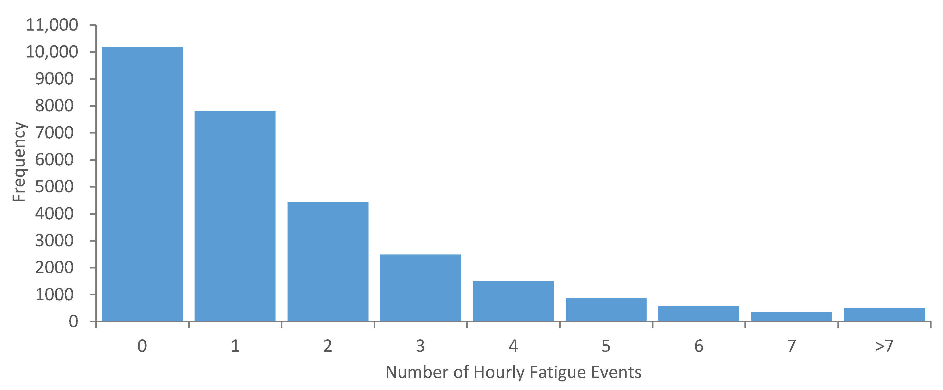
To illustrate the relationship between hourly data and the frequency of fatigue events, their distribution is provided in Figure 3. This right-skewed distribution shows that more than 50% of the hours contain at least one fatigue event. This suggests that further exploration is needed to identify the variables contributing to the range of hourly fatigue events. Therefore, a second model with hourly aggregated data is developed, which will be introduced in the model section. In addition, Figure 4a shows that night shifts contain significantly more events compared to day shifts. Moreover, the average event counts by month indicate a seasonality effect, with lower rates of fatigue in spring and higher rates in summer and winter (Figure 4b). To summarize, the above explorations demonstrate that some variables, such as shift type, time of day and worked hours, have effects on fatigue. At the same time, the findings suggest that advanced approaches will be required to model fatigue events.
Next, we conduct an exploration of the influence of environmental variables on operator fatigue. Figure 5 illustrates the monthly average ambient temperature and monthly fatigue events per person, without any clear pattern. Thus, there appears to be no obvious correlation between temperature and fatigue events in this plot. Therefore, for further exploration, weather data are added as independent variables to the model.
The main purpose of the above analyses was to explore relationships between fatigue events and variables contained in the existing data sets. From our initial data analyses, fatigue appears to have some relationship with variables such as weather, shift type, time of day, etc. These analyses introduce more variables for the purpose of the modeling and data aggregating methods. The full list of variables is shown in Table 3. However, these preliminary analyses are not able to identify a pattern of fatigue based on these variables, although they are able to provide a critical insight into the data. The literature shows that fatigue is a complex issue and different psychological and physiological variables influence fatigue in workers [2]. Considering the limitations of the above analytical approaches, we use machine learning (ML) approaches as an alternative to explore the data set to elucidate relationships that are not easily identifiable. Because the above analyses show that shift type and hour of day appear to have significant effects on the fatigue of haul truck drivers, data were aggregated by shift and hour to create two different models. One approach involves fatigue prediction using the shift-based data, and the other uses hourly data to predict fatigue. The next section presents the modeling approach.

3.3. Machine Learning Model

Figure 6 presents the procedure and methods of the modeling steps involved in the development of the machine learning model. The process involved the following steps:
  • Data collection;
  • Data pre-processing;
  • Data engineering;
  • Training model;
  • Testing model;
  • Model evaluation;
  • Making predictions.

3.3.1. Random Forest Regression Algorithm

The machine learning model selected for this analysis is a random forest (RF) regression algorithm. Random forest algorithms were chosen for their tendency to generalize well to a wide variety of problems, their rapid speed of training and because they are a key feature of many well-known machine learning solutions. Another key benefit of using random forests is the tooling that has been built in recent years to help researchers to gain insights into what has long been thought of as the black box of machine learning. These new analytical tools allow researchers to see the features that the model relies upon the most in order to make predications and determine how marginal changes in these features impact the predicted outcomes [30,31].
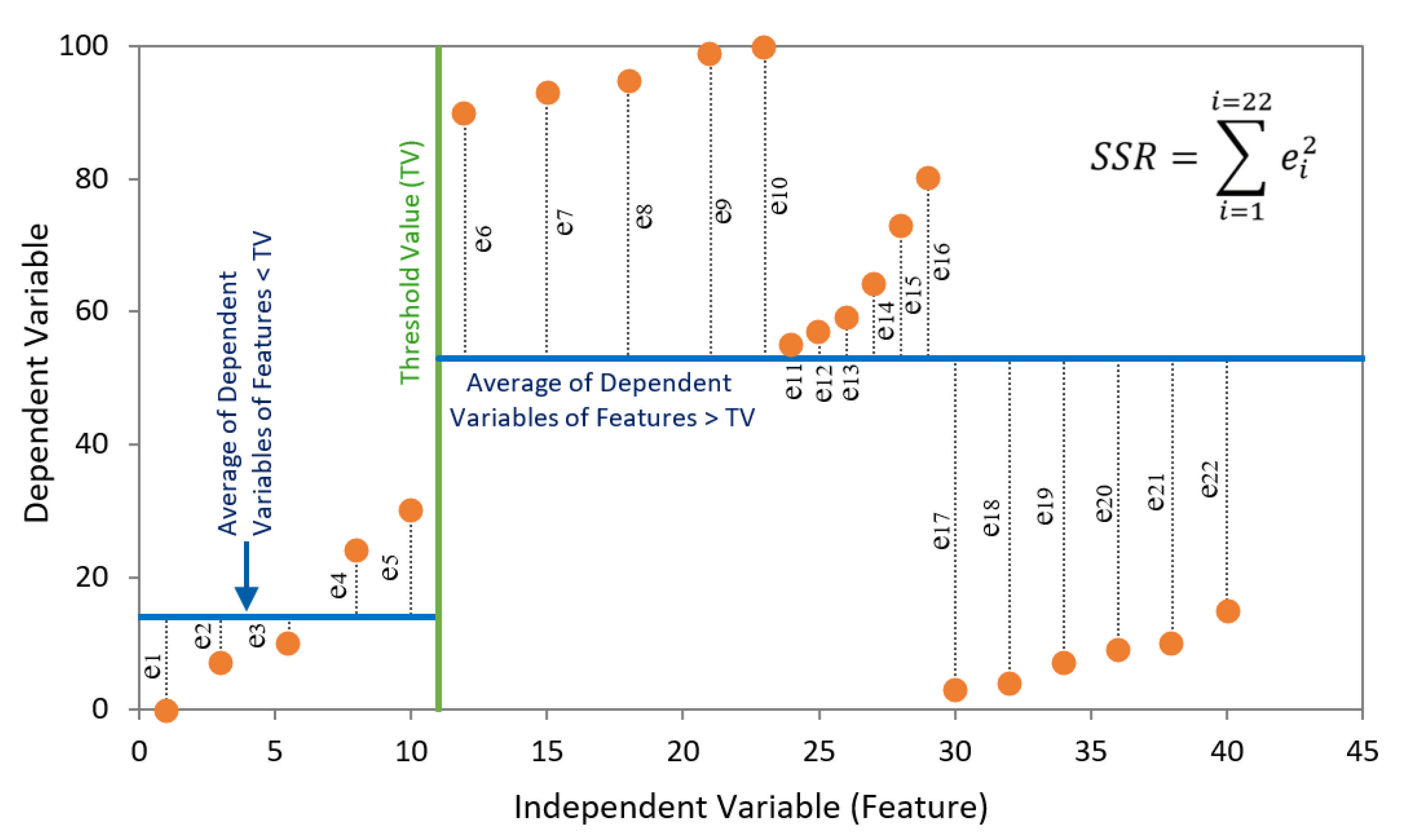
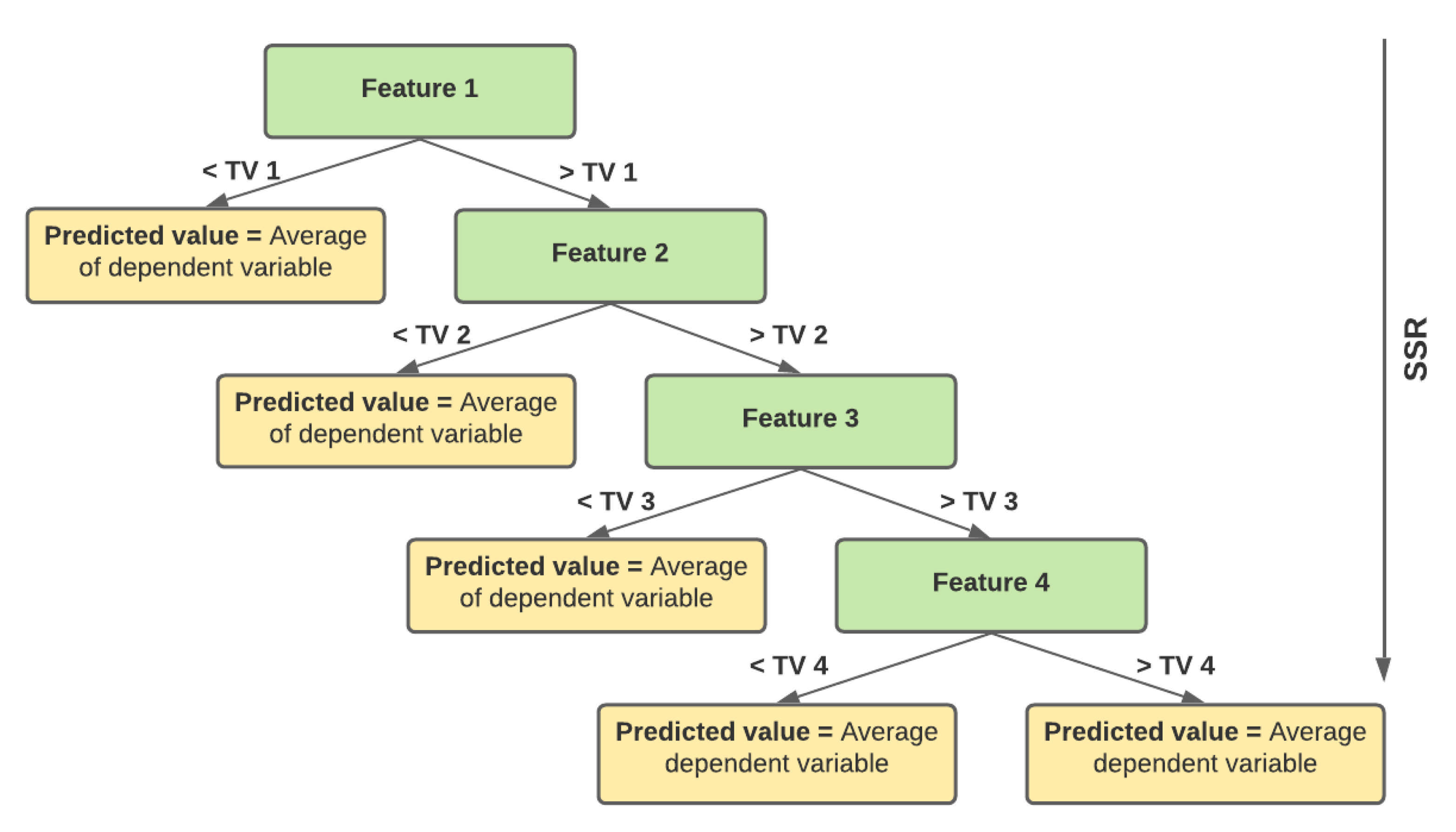
When data are not linearly scattered, a regression tree, which is a type of decision tree, can be used. In this type of decision tree, each leaf presents a threshold value (TV) for each feature of the model. For the purpose of finding the best decision tree, the model tries to find the best threshold value for each feature (independent variable) by finding the minimum sum of square residuals (SSR). SSR is the sum of the squared difference of each prediction value and actual value (Figure 7). For models with more than one feature, the decision tree root is the feature with the lowest SSR. Figure 8 represents an example of a random forest regression decision tree with five features.
A random forest regression algorithm is an ensemble of randomized regression trees. The random forest algorithm creates bootstrap samples from the original data. Bootstrapping is a procedure that resamples a single data set to create many simulated samples. For each of the bootstrap samples, the algorithm increases a classification or regression tree. This algorithm chooses a random sample of the predictors and selects the best split among variables. Then it predicts new data by aggregating the predictions of the trees. Models can estimate the error rate based on the training data by each bootstrap iteration [30,31].

3.3.2. Model

Two models were created using available data subsets as dependent variables. For the shift-based model, the dependent variable was the number of fatigue events in a 12 h shift, which was normalized to scheduled haulage hours in the shift (labor hours). For the hourly-based model, the dependent variable was the number of fatigue events in an hour, which was normalized to scheduled haulage hours (labor hours). All independent variables in these models, also known as features, are representations of the mine’s operation as represented in the data sets. These features contain values such as the average production, average temperature and equipment alarm (see Table 3).
For this model, data were divided into two sets: 80% constituted the training data set and 20% constituted the validation data set. The goal of these models was to determine the features that can predict fatigue in such a way that minimizes RMSE. In these models, only data subsets with micro-sleeps and drowsiness containing fatigue were modeled. From 151,432 possible events, only 44,953 contained micro-sleep and drowsiness in the data sets to train and validate the random forest algorithm. After exploratory data analysis, this study focused on refining models to predict the fatigue of the operator.
The independent variables (features) in these models were minimally engineered. Then, possible sample counts, means, sums, mins and maxes were used without combining multiple fields from the underlying tables. The goal of these models was to predict fatigue as well as the possibility of including all available feature sets, such as the hour of the day, shift, month of the year, ambient temperature, wind speed, precipitation, etc. Data for these models were constrained to the number of days contained in the fatigue data, which was a dependent variable. Thus, the models were created using data from 1 January 2014 to 9 August 2017.

3.3.3. Evaluating Model Performance

One way to evaluate the model performance is out-of-bag error or OOB. The out-of-bag set includes data not chosen in the sampling process when initially building a random forest. The out-of-bag (OOB) error is the average error for each calculated prediction from the trees not contained in the respective sample. Here, we used the Random Forest python package, which can generate two optional information values, a value of the importance of the predictor variables (feature importance) and a value of the internal structure of the data (the proximity of different data points to one another) [30].
Next, the performance of the model was evaluated using the root mean squared errors (RMSE) and coefficients of determination (R2). The coefficient of determination is the best method to compare models that are trained using different dependent variables. Both RMSE and coefficients of determination are important means of measuring performance between models trained to predict the same dependent variable. The reason that R2 should be used when comparing models trained on different dependent variables is that the coefficient of determination is normalized to the mean of the dependent variable for each model.

3.3.4. Model Generalization

When creating machine learning models, it is important to ensure that the predictions are generalizable to data that the model was not trained on. A model that has a very low training error but a very high validation error is considered not to generalize well. This scenario is known as overfitting [32]. The most common method to ensure that a model has not been overfit is splitting data into training and validation sets. The model learns its parameters from the training data set. The performance of the trained model is then determined by how well it predicts the outcomes of the validation data set. The hyperparameters of the model can then be tuned by the developer, and the model is retrained to improve its performance against the validation data set. Hyperparameters are the values that define the model and cannot be learned from data; they are set by the developer of the machine learning algorithm (number of estimators, max number of features, etc.). The number of estimators and the max number of features for the best model here are 1000 and sqrt (number of features), respectively. For each model here, the data sets were split into training and validation sets. In this study, due to a lack of sufficient data for a double hold-out (test set), there is only a validation set.

3.3.5. Feature Importance

Feature importance is the process of ranking the individual elements of a machine learning model according to their relative importance to the accuracy of that model [33,34]. Feature importance is a means of determining the features that have the greatest magnitude of effect in a model. Features that have a high feature importance value have a greater impact on the model. Feature importance refers to a technique to assess the scores of independent variables to a predictive model. It indicates the relative importance of each independent variable (feature) when making a model prediction. These scores can be used to better understand the data and model and reduce the number of input features. The relative scores of feature importance can highlight which features are more useful to predict fatigue and, conversely, which features are the least helpful to predict fatigue. This may be used as the basis for gathering more or different data. Moreover, it shows that the model has been fit to the most important features. In addition, feature importance can be used to improve a predictive model. It can be used to eliminate the features with the lowest scores or retain those with the highest scores. Therefore, it can help to select features and speed up the modeling process.

4. Results

Differences between the two models were found after the analyses. The hourly-based model does not perform as well as the shift-based model according to their R2 and RMSE. The best model used the shift-based data to predict fatigue. Below, we discuss feature importance and drop column tools to examine the feature set of the shift-based model.
In Table 4, the results of the best performed model are displayed. The best-performing model predicted fatigue events across the site, with an R2 value of 0.36 and RMSE value of 0.006. All other models were deemed to have values too low to warrant further exploration using this feature set. The best model used the shift-based data to predict fatigue. Below, we discuss feature importance and drop column tools to examine the feature set of the shift-based model.

4.1. Feature Importance of Best-Performing Model

Generally, feature importance provides a score that identifies the value of each feature in creating the random forest model. Features that have a greater effect on key decisions have higher relative importance. Table 5 shows the most important features and their values for the fatigue event prediction model (shift-based model) with the best performance.
The shift type (day/night shift) variable has the strongest effect on the model. Next, the amount of unscheduled downtime of the equipment of the whole mine for a shift affected the model. “Unscheduled downtime” is when a piece of equipment goes down for maintenance reasons in an unplanned situation. Other factors that have effects on fatigue are production variables. These outcomes corroborate with the initial data analyses regarding the effects of day shifts and night shifts on the fatigue of workers. It also demonstrates that production and equipment alarm variables such as equipment downtime can aid in predicting the occurrence of fatigue events. Moreover, weather variables such as maximum and average temperature can increase the rate of fatigue events among workers.

4.2. Drop-Column Feature Importance

With large data sets, there is always a risk of having variables that are covariates or have co-dependences. Random forest tools recognize that this risk exists and include mechanisms to address it, which can assess the individual effects of each feature on the model. Co-dependencies stem from the fact that the trees are not independent since they are sampled from the same data in the process of making the RF model. It is important to see how the model works without individual features and how each feature impacts the model, whether positively or negatively. Instead of carrying out different iterations, random forest algorithms have a built-in tool which runs models with fewer features and tracks the models’ performance. This is achieved by dropping out each column (or feature) from the model, retraining the entire model and then comparing the score with the base score. Negative values show features that improve the model when removed. Positive values show features that weaken the model when removed. Values that are close to zero tend to indicate features that are correlated with other features; thus, removing them makes little difference in the model’s ability to find relationships using the correlated variables. In Table 6, the ten most and ten least important features are displayed.
As shown in Table 6, shift type has the strongest effect on the model, followed by some production and alarm variables, as indicated by their feature importance score. This score shows that dropping, for example, shift type, from the features, causes the performance of the model (R2) to drastically decrease by 0.2922. On the other hand, eliminating the mine load capacity percentage increases the performance of the model by 0.0325.

4.3. ICE Plot

Another tool to visualize how marginal changes in features affect the predictions of the model is an individual conditional expectation (ICE) plot. An ICE plot identifies the dependence of the prediction on a feature for each instance independently. It generates one line per instance, which can be compared to one line overall in partial dependence plots. A partial dependence plot (PDP) is the average of the lines of an ICE plot. The value of a line or model score is compared when all other features are kept the same. The result is a set of points for an instance with a feature value from the grid and the respective predictions [35]. ICE plots for the four top features are displayed in Figure 9 and ICE plots of ten top features are provided in Appendix A. They show how the models’ predictions change depending on marginal changes to the top features. For instance, they illustrate that the prediction difference in the model for shift of day decrease from the day shift to the night shift. The ICE plot of unscheduled downtime count shows that the prediction difference of the model for a small amount of unscheduled downtime of the equipment is not high, but it starts to increase after 40 counts of unscheduled downtime of the equipment. Moreover, the prediction difference of the model for mine measured production is small, but it increases after 300,000 tons of production. Therefore, looking at the marginal changes in the top features offers insights into how marginal changes affect the model prediction.

4.4. Comparison

Table 7 shows the top features from two different generated models. Of the models that were run, the best performance was demonstrated by the shift-based fatigue model that is used to predict fatigue events based on shift data. This model achieved an R2 value of 0.36, which is reasonably high for the prediction of outcomes that are the result of very complex interactions. Fatigue is a complex issue and can occur for different psychological and physiological reasons; therefore, it is difficult to predict it with high accuracy.
Another model, which is based on the hourly aggregated fatigue occurrence, identifies that the time of day helps to predict the fatigue as expected, since this is one of the top features in the hourly-based model. Moreover, ambient temperature has a notable effect on fatigue, which is evidenced by the hourly-based model; however, it is obvious that temperature is linked to the time of day. More work is needed to assess the potential role of air conditioning in this. In addition to time and weather factors, some production and equipment health alarm variables have effects on the fatigue of haul truck drivers, as the hourly-based model shows (see Table 7).

5. Discussion

The model output identifies the variables that have the greatest impact on all fatigue events. Table 8 illustrates the most important features and their data sources. The results confirm our existing understanding of fatigue and offer some interesting insights into additional factors that potentially cause fatigue. While it is not surprising that shift type causes fatigue, it is interesting that maintenance processes such as unscheduled downtime and production rates, as well as other operational variables, can affect fatigue among haul truck drivers. Having identified these additional predictors for fatigue, these indicators can be used by managers to prioritize safety management efforts. The ICE plots show how marginal changes to specific variables affect the model. Therefore, they can be potentially used as thresholds for KPIs. For example, if the mine is approaching a value of 40 for unscheduled downtime, a higher risk of fatigue is indicated.
In many fields of science, it is difficult to consider models that achieve R2 values of high magnitude. Since fatigue is a complex issue, finding a comprehensive model with a high R2 is challenging. However, the methodology and future iterations could provide beneficial insights. The finding that 36% of fatigue events can be explained by shift type, weather and operational data indicates that 64% of the variance can be attributed to factors that we currently are not modeling. Therefore, the next step in fatigue modeling would be exploring additional contributors to operator fatigue. In this study, the mine’s data have been aggregated according to shift or hour, but future models could examine fatigue in a more individualistic way. Deeper integration of the data sets upon individual operators could be one way of accomplishing this. Additional factors such as an individual’s habits and sleep patterns could also provide another level to the model and would give a more detailed view of the fatigue of the workers.
From the perspective of health and safety management, the most important features found in this study can be considered potential leading indicators (ALIs) to reduce fatigue. The surprising finding of unscheduled equipment downtime events is an aspect that needs to be explored further. Process disruption’s impact on fatigue was one finding that was consistent with the study by Drews et al. (2020) [2]. More research from a health and safety perspective is needed to understand why some of the alarm and production variables of different fleets have a greater effect on fatigue. However, fitness for duty could be one reason behind the different fatigue events for different fleets. Mining companies can use these indicators to anticipate increases in fatigue and to potentially mitigate fatigue. These model outcomes can be utilized to implement health and safety policies, training programs and mitigation practices. If mine operations can identify the times and shift types that are more susceptible to fatigue, specific strategies could be implemented, such as mandatory break times for the operators and supervisory support during this time. Management can also train the operators to be more alert at specific times of the day and during specific shifts. They also can train them to be more aware of how fitness can decrease fatigue. The models’ output shows that ambient temperature has also significant effects on the fatigue of haul truck drivers. This also must be studied further to understand the degree to which this factor influences specific individuals’ fatigue states.
Moreover, the hourly-based model results provide an understanding of the effects of the variables that impact fatigue for health and safety management. It demonstrates that a leading indicator to predict fatigue is the time of day. Therefore, special attention and planning is required for those times with a higher risk of fatigue. All of these outcomes can be considered when prioritizing tasks by health and safety management.

6. Limitations and Future Work

This study shows the application of machine learning in health and safety management using operational data sets of mining operations. The findings of this study confirm that fatigue is caused by a wide variety of factors and many are likely very difficult to quantify, but there may be a small but impactful percentage of factors that can be quantified. Fatigue prediction is a matter of predicting the complex interactions between human behavior and the ever-changing work environments at mines. In the social sciences, it is very common to see situations where a low R2 value captures relationships that quantify a relatively high amount of variance in a complex relationship [36]. Individual worker data can be added to the model to increase the accuracy of the prediction model, since only operational data and weather data are utilized in these models.
In all of the models developed, the training scores are substantially better than the validation scores. This is most often attributable to overfitting of the model, but in this case, it is likely largely due to the difficultly in generalizing a model that can predict fatigue due to the complex psychological and physiological factors associated with fatigue. This line of research will become more important as the fitness for duty of equipment operators takes on greater significance in scheduling operator work shifts.
Even when using a fairly simple model with a small data set, the best-performing model in this study is able to achieve excellent results. Many refinements were made to the models during this study, but there are many avenues of exploration that could yield even stronger predictive models. Some key areas to explore in future models could include:
  • Looking at individual fatigue events instead of the aggregated fatigue events;
  • Using a machine learning method that can model more complex relationships, such as a neural network;
  • Increasing the size of the training data set—this could be accomplished by adding more data either from the same mine or from another mine;
  • Creating common naming conventions between data sets so that they can be linked by location, operator and equipment;
  • Adding more complex features such as the sleep pattern, health condition, fitness or diet of the operator;
  • Adding features that represent information collected during time periods prior to when the fatigue occurred, such as downtime or production on the previous day;
  • Adding some features related to the working schedule of the operator in terms of fatigue at the time and the day or week before;
  • Exploring more details of each feature to reduce the number of features that have a lower impact on fatigue.

Author Contributions

Conceptualization, E.T. and W.P.R.; methodology, E.T., W.P.R. and T.M.; software, E.T. and T.M.; validation, W.P.R., E.T. and F.A.D.; formal analysis, E.T.; investigation, E.T.; resources, W.P.R.; data curation, E.T. and T.M.; writing—original draft preparation, E.T.; writing—review and editing, E.T., W.P.R. and F.A.D.; visualization, E.T.; supervision, W.P.R.; project administration, W.P.R.; funding acquisition, W.P.R. All authors have read and agreed to the published version of the manuscript.

Funding

Funding for the project was provided by the National Institute for Occupational Safety and Health (NIOSH) with grant number 75D30119C05500.

Data Availability Statement

The data presented in this study are not publicly available due to confidentiality.

Acknowledgments

We would like to express our gratitude to the National Institute for Occupational Safety and Health (NIOSH) for the funding, as well as the mining company, its management and all of the people supporting this research.

Conflicts of Interest

On behalf of all authors, the corresponding author states that there is no conflict of interest.

Appendix A

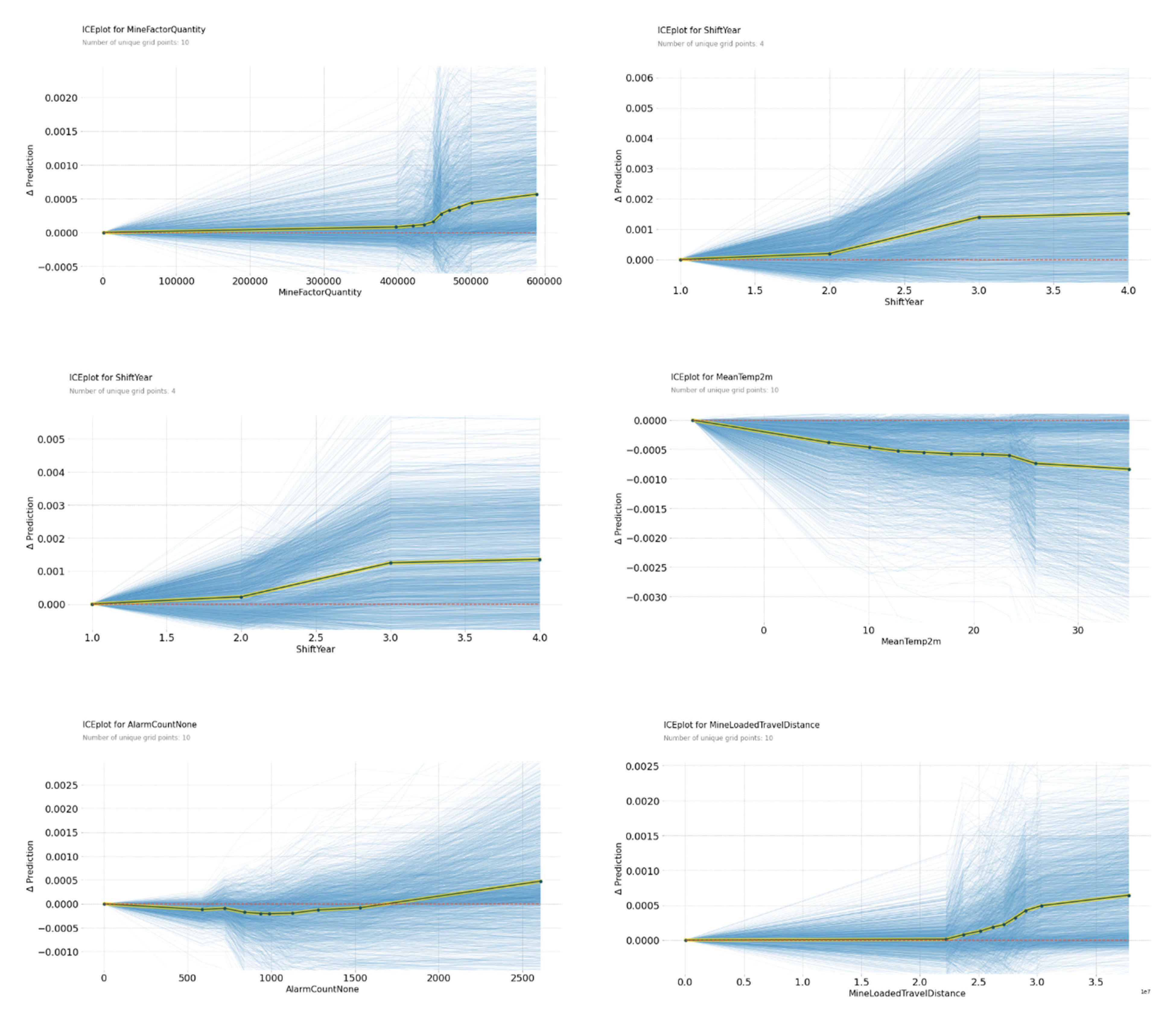
The ICE plots of the top ten features from the shift-based model are presented in Figure A1.
Figure A1. ICE plots of the top ten features (Blue lines identify the dependence of the prediction on a feature for each instance independently, and yellow line is PDP which shows the average of the blue lines).
Minerals 11 00621 g0a1aMinerals 11 00621 g0a1b

References

  1. Bauerle, T.; Dugdale, Z.; Poplin, G. Mineworker fatigue: A review of what we know and future directions. Min. Eng. 2018, 70, 1–19. [Google Scholar]
  2. Drews, F.A.; Rogers, W.P.; Talebi, E.; Lee, S. The Experience and Management of Fatigue: A Study of Mine Haulage Operators. Min. Metall. Explor. 2020, 37, 1837–1846. [Google Scholar] [CrossRef]
  3. Dawson, D.; Searle, A.K.; Paterson, J.L. Look before you (s)leep: Evaluating the use of fatigue detection technologies within a fatigue risk management system for the road transport industry. Sleep Med. Rev. 2014, 18, 141–152. [Google Scholar] [CrossRef] [PubMed]
  4. Briggs, C.; Nolan, J.; Heiler, K. Fitness for Duty in the Australian Mining Industry: Emerging Legal and Industrial Issues; 186487421X; Australian Centre for Industrial Relations Research and Teaching: Sydney, NSW, Australia, 2001; pp. 1–52. [Google Scholar]
  5. Parker, T.W.; Warringham, C. Fitness for work in mining: Not a ‘one size fits all’ approach. In Proceedings of the Queensland Mining Industry Health & Safety Conference, Brookfield, QLD, Australia, 4–7 August 2004. [Google Scholar]
  6. Hutchinson, B. “Fatigue Management in Mining—Time to Wake up and Act”, Optimize Consulting. 2014. Available online: http://www.tmsconsulting.com.au/basic-fatigue-management-in-mining/ (accessed on 25 January 2020).
  7. Pelders, J.; Nelson, G. Contributors to Fatigue of Mine Workers in the South African Gold and Platinum Sector. Saf. Health Work 2019, 10, 188–195. [Google Scholar] [CrossRef]
  8. Cavuoto, L.; Megahed, F. Understanding fatigue and the implications for worker safety. In Proceedings of the ASSE Professional Development Conference and Exposition, Atlanta, GA, USA, 26 June 2016. [Google Scholar]
  9. Talebi, E.; Roghanchi, P.; Abbasi, B. Heat management in mining industry: Personal risk factors, mitigation practices, and industry actions. In Proceedings of the 17th North American Mine Ventilation Symposium, Montreal, QC, Canada, 28 April–1 May 2019. [Google Scholar]
  10. Talebi, E.; Sunkpal, M.; Sharizadeh, T.; Roghanchi, P. The Effects of Clothing Insulation and Acclimation on the Thermal Comfort of Underground Mine Workers. Min. Metall. Explor. 2020, 37, 1827–1836. [Google Scholar] [CrossRef]
  11. Yung, M. Fatigue at the Workplace: Measurement and Temporal Development. Ph.D. Thesis, University of Waterloo, Waterloo, ON, Canada, 2016. [Google Scholar]
  12. Tufano, P. Who manages risk? An empirical examination of risk management practices in the gold mining company. J. Financ. 1996, 51, 1097–1137. [Google Scholar] [CrossRef]
  13. Wegerich, S.W.; Wolosewicz, A.; Xu, X.; Herzog, J.P.; Pipke, R.M. Automated Model Configuration and Deployment System for Equipment Health Monitoring. U.S. Patent No. 7,640,145 B2, 29 December 2009. [Google Scholar]
  14. Hinze, J.; Thurman, S.; Wehle, A. Leading indicators of construction safety performance. Saf. Sci. 2013, 51, 23–28. [Google Scholar] [CrossRef]
  15. Poh, C.Q.X.; Ubeynarayana, C.U.; Goh, Y.M. Safety leading indicators for construction sites: A machine learning approach. Autom. Constr. 2018, 93, 375–386. [Google Scholar] [CrossRef]
  16. Hallowell, M.R.; Hinze, J.W.; Baud, K.C.; Wehle, A. Proactive construction safety control: Measuring, monitoring, and responding to safety leading indicators. J. Constr. Eng. Manag. 2013, 139, 1–8. [Google Scholar] [CrossRef]
  17. Guo, B.H.W.; Yiu, T.W. Developing Leading Indicators to Monitor the Safety Conditions of Construction Projects. J. Manag. Eng. 2016, 32, 1–14. [Google Scholar] [CrossRef]
  18. Toellner, J. Improving Safety & Health Performance: Identifying & Measuring Leading Indicators. Prof. Saf. J. 2011, 46, 42–47. [Google Scholar]
  19. Grabowski, M.; Ayyalasomayajula, P.; Merrick, J.; McCafferty, D. Accident precursors and safety nets: Leading indicators of tanker operations safety. Marit. Policy Manag. 2007, 34, 405–425. [Google Scholar] [CrossRef]
  20. Hopkins, A. Thinking About Process Safety Indicators. In Proceedings of the Oil and Gas Industry Conference, Manchester, UK, 4–6 November 2007. [Google Scholar]
  21. Hale, A. Why safety performance indicators? Saf. Sci. 2009, 47, 479–480. [Google Scholar] [CrossRef]
  22. Costin, A.; Wehle, A.; Adibfar, A. Leading indicators—a conceptual IoT-based framework to produce active leading indicators for construction safety. Safety 2019, 5, 86. [Google Scholar] [CrossRef] [Green Version]
  23. Kononenko, I.; Kukar, M. Machine Learning and Data Mining; Woodhead Publishing: Cambridge, UK, 2007; pp. 1–36. [Google Scholar]
  24. Thibaud, M.; Chi, H.; Zhou, W.; Piramuthu, S. Internet of Things (IoT) in high-risk Environment, Health and Safety (EHS) industries: A comprehensive review. Decis. Support Syst. 2018, 108, 79–95. [Google Scholar] [CrossRef]
  25. Molaei, F.; Rahimi, E.; Siavoshi, H.; Afrouz, S.G.; Tenorio, V. A Comprehensive Review on Internet of Things (IoT) and its Implications in the Mining Industry. Am. J. Eng. Appl. Sci. 2020, 13, 499–515. [Google Scholar] [CrossRef]
  26. Shahmoradi, J.; Talebi, E.; Roghanchi, P.; Hassanalian, M. A comprehensive review of applications of drone technology in the mining industry. Drones 2020, 4, 34. [Google Scholar] [CrossRef]
  27. Tixier, A.J.P.; Hallowell, M.R.; Rajagopalan, B.; Bowman, D. Application of machine learning to construction injury prediction. Autom. Constr. 2016, 69, 102–114. [Google Scholar] [CrossRef] [Green Version]
  28. Lingard, H.; Hallowell, M.; Salas, R.; Pirzadeh, P. Leading or lagging? Temporal analysis of safety indicators on a large infrastructure construction project. Saf. Sci. 2017, 91, 206–220. [Google Scholar] [CrossRef]
  29. Cheng, T. When Artificial Intelligence Meets the Construction Industry. Available online: https://www.gxcontractor.com/equipment/article/13031944/when-artificial-intelligence-meets-the-construction-industry (accessed on 25 May 2018).
  30. Liaw, A.; Wiener, M. Classification and regression by random Forest. R News 2002, 2, 18–22. [Google Scholar]
  31. Breiman, L. Random Forests. Mach. Learn. 2001, 45, 5–32. [Google Scholar] [CrossRef] [Green Version]
  32. Segal, M.R. Machine Learning Benchmarks and Random Forest Regression; Technical Report for Center for Bioinformatics and Molecular Biostatistics; University of California: San Francisco, CA, USA, April 2003. [Google Scholar]
  33. Heaton, J.; McElwee, S.; Fraley, J.; Cannady, J. Early stabilizing feature importance for TensorFlow deep neural networks. In Proceedings of the 2017 International Joint Conference on Neural Networks (IJCNN), Anchorage, AK, USA, 14–19 May 2017; pp. 4618–4624. [Google Scholar]
  34. Menze, B.H.; Kelm, B.M.; Masuch, R.; Himmelreich, U.; Bachert, P.; Petrich, W.; Hamprecht, F.A. A comparison of random forest and its Gini importance with standard chemometric methods for the feature selection and classification of spectral data. BMC Bioinform. 2009, 10, 213. [Google Scholar] [CrossRef] [Green Version]
  35. Molnar, C. Interpretable Machine Learning, A Guide for Making Black Box Models Explainable. Available online: https://christophm.github.io/interpretable-ml-book/ (accessed on 25 March 2021).
  36. Minitab Blog Editor. Regression Analysis: How Do I Interpret R-Squared and Assess the Goodness-of-Fit? Available online: https://blog.minitab.com/en/adventures-in-statistics-2/regression-analysis-how-do-i-interpret-r-squared-and-assess-the-goodness-of-fit (accessed on 20 February 2021).
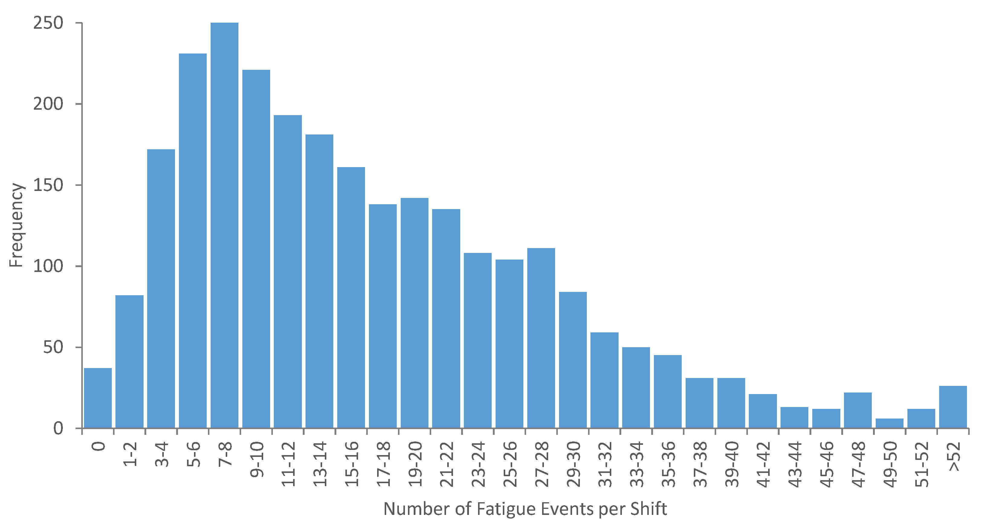
Figure 1. Fatigue events per shift frequency.
Minerals 11 00621 g001
Figure 2. Hourly fatigue events and average hourly production.
Minerals 11 00621 g002
Figure 3. Hourly fatigue events frequency.
Minerals 11 00621 g003
Figure 4. (a) Fatigue events per shift; (b) Average monthly fatigue events.
Minerals 11 00621 g004
Figure 5. Monthly fatigue events per person vs. average temperature.
Minerals 11 00621 g005
Figure 6. Procedure diagram for the prediction of fatigue using random forest regression algorithm.
Minerals 11 00621 g006
Figure 7. Finding TV and SSR for random data (e or error is difference of each predicted value (average value) and actual value, and i is the feature number).
Minerals 11 00621 g007
Figure 8. Schematic random forest regression decision tree.
Minerals 11 00621 g008
Figure 9. ICE plots of the top three features (Blue lines identify the dependence of the prediction on a feature for each instance independently, and yellow line is PDP which shows the average of the blue lines).
Minerals 11 00621 g009
Table 1. Data sets’ details.
Data SourceKey FactorsDate Range
Fatigue monitoringOperator drowsiness, micro-sleeps, etc.2014–2017
Time and AttendanceHours worked, shift worked, etc.2014–2017
Fleet management system
(production and status)
Production cycles, faulty equipment, delayed equipment, etc.2014–2017
Equipment health alarms and eventsNotification of equipment abuse, use of equipment, etc.2014–2017
Weather conditionsTemperature, wind speed, wind direction, change,
precipitation, relative humidity, etc.
2014–2017
Table 2. Count of days and percentage of total days by fatigue type.
Fatigue Event TypeAverage Number of
Events per Day
Days with Fatigue EventsPercentage of Days with
Fatigue
Percentage of Fatigue Events
Micro-Sleep with Stable Head13131398%40%
Other Eye Closure (Drowsiness)20132799%60%
Table 3. List of the variables based on the data source.
Data SourceVariablesData Type and Example Data
Time and AttendanceShift IDInteger (1 to 4140)
Shift of Day (shift type)Categorical Integer (0 and 1)
Crew NameCategorical Integer (1 to 4)
Days OnInteger (0 to 4)
YearInteger (2014 to 2017)
MonthInteger (1 to 12)
WeekInteger (1 to 54)
DayInteger (1 to 31)
Day of weekInteger (1 to 7)
Day of yearInteger (1 to 365)
Hour of dayFloat (0 to 24)
Shift is end of monthCategorical Integer (0 and 1)
Shift is start of monthCategorical Integer (0 and 1)
Shift is end of quarterCategorical Integer (0 and 1)
Shift is start of quarterCategorical Integer (0 and 1)
Shift is end of yearCategorical Integer (0 and 1)
Shift is start of yearCategorical Integer (0 and 1)
Fleet management system
(production and status)
Mine Production FactorInteger (1335 to 589,201)
Mine Loaded Travel DistanceInteger (37,884 to 37,797,788)
Mine Measured ProductionInteger (0 to 430,812)
Mean Measured Production (broken down by fleet, creating 8 variables)Float (0 to 413.83)
Mine Load Capacity PercentageFloat (0 to 1)
Mean Load Capacity Percentage (broken down by fleet, creating 8 variables)Float (0 to 1)
Mean Loaded Travel DistanceFloat (3735.2 to 13,711.66)
Mean Loaded Travel LiftFloat (272.25 to 1083.29)
Mean Loaded Travel Lift DistanceFloat (3735.2 to 13,711.66)
St Dev Loaded Travel DistanceFloat (604.55 to 16,118.27)
WeatherMean Barometric PressureFloat (0 to 25.1)
Mean PrecipitationFloat (0 to 439.1)
Mean Temperature (2 m)Float (−6.8 to 34.8)
Min Barometric PressureFloat (0 to 25.01)
Min PrecipitationFloat (0 to 29.71)
Min Temperature (2 m)Float (−8.4 to 30.44)
Max Barometric PressureFloat (0 to 25.1)
Max PrecipitationFloat (0 to 756.9)
Max Temperature (2 m)Float (−4.435 to 36.82)
Sum PrecipitationFloat (0 to 5269.17)
Equipment health alarms and eventsBoth Alarm CountInteger (0 to 632)
Electrical Alarm CountInteger (0 to 892)
Lockout Alarm CountInteger (0 to 35)
Maintenance Alarm CountInteger (0 to 1094)
Mechanical Alarm CountInteger (0 to 1753)
None Alarm CountInteger (0 to 2608)
Normal Alarm CountInteger (0 to 121)
Operational Alarm CountInteger (0 to 819)
Undetermined Alarm CountInteger (0 to 1282)
Scheduled Down CountInteger (0 to 85)
Unscheduled Down CountInteger (0 to 141)
Operational Delay CountInteger (0 to 1126)
Operational Down CountInteger (0 to 80)
Ready Non-Production CountInteger (0 to 977)
Ready Production CountInteger (0 to 1322)
Fatigue
monitoring system
Drowsiness and Micro-Sleep Fatigue Events Count (Normalized)Float (0 to 1)
Table 4. Refined model performance results.
ModelRoot Mean Squared Error (RMSE)Coefficient of Determination R2
TrainingValidationTrainingValidationOOB
Shift-based model0.0020.0060.930.360.47
Table 5. Permutation importance of features for shift-based model (most important features).
Data CategoryDependent VariablesFeature Importance Score
Time and AttendanceShift type (day or night shift)0.1650
Equipment health alarms and eventsUnscheduled downtime count0.0588
Fleet management system
(production and status)
Mine load capacity percentage0.0297
Mine measured production0.0293
Mine production factor0.0248
Time and AttendanceYear0.0245
WeatherMean temperature (2 m)0.0235
Equipment health alarms and eventsNone alarm count0.0230
Fleet management system
(production and status)
Mine loaded travel distance0.0226
Mean measured production of haul truck (CAT 793D)0.0226
WeatherMaximum temperature (2 m)0.0223
Equipment health alarms and eventsReady production count0.0222
Mechanical alarm count0.0215
Fleet management system
(production and status)
Mean load capacity percentage of haul truck (CAT 793D)0.0213
Mean measured production of haul truck (CAT 793C)0.0211
Mean loaded travel distance0.0209
Mean measured production of haul truck (CAT 793B)0.0209
Mean load capacity percentage of haul truck (CAT 793C)0.0208
Mean load capacity percentage of haul truck (CAT 793B)0.0207
Equipment health alarms and eventsScheduled down count0.0206
Table 6. Drop-column importance for the best model.
Dependent VariablesFeature Importance Score
Shift type (day or night) 0.2922
Unscheduled downtime count 0.0317
Mechanical alarm count0.0235
Day on0.0225
Day of week 0.0205
Mean measured production of haul truck (CAT 797F)0.0139
Shift is end of year0.0129
Electrical alarm count0.0129
Mine measured production0.0127
Undetermined alarm count0.0125
None alarm count−0.0022
Mean loaded travel distance−0.0025
Mean load capacity percentage of haul truck (CAT 793D)−0.0031
Year−0.0034
Mean Temperature (2 m)−0.0073
Mean load capacity percentage of haul truck (CAT 793B)−0.0073
Mean loaded travel lift distance −0.0074
Maintenance alarm count −0.0083
Mean loaded travel lift −0.0119
Mine load capacity percentage−0.0325
Table 7. Comparison of the top features for hourly-based and shift-based models.
RankingsShift-Based ModelHourly-Based Model
1Shift type (day or night shift)Mean temperature (2 m)
2Unscheduled downtime countHour of day
3Mine load capacity percentageMean measured production of haul truck (CAT 793B)
4Mine measured productionMean measured production of haul truck (CAT 793D)
5Mine production factorNone alarm count
6YearSt Dev loaded travel distance
7Mean temperature (2 m)Mean barometric pressure
8None alarm countMaintenance alarm count
9Mine loaded travel distanceUndetermined alarm count
10Mean measured production of haul truck (CAT 793D)Mine production factor
Table 8. Top features by data classification.
Data CategoryFeature RankFeature
Time and attendance1Shift of day (day or night)
6Year
Fleet management system
(production and status)
3Mine load capacity percentage
4Mine measured production
5Mine production factor
9Mine loaded travel distance
10Mean measured production of haul truck (CAT 793D)
14Mean load capacity percentage of haul truck (CAT 793D)
15Mean measured production of haul truck (CAT 793C)
16Mean loaded travel distance
17Mean measured production of haul truck (CAT 793B)
18Mean load capacity percentage of haul truck (CAT 793C)
19Mean load capacity percentage of haul truck (CAT 793B)
Equipment health alarms and events2Unscheduled down count
8None alarm count
12Ready production count
13Mechanical alarm count
20Scheduled downtime count
Weather7Mean temperature (2 m)
11Maximum temperature (2 m)
Publisher’s Note: MDPI stays neutral with regard to jurisdictional claims in published maps and institutional affiliations.