Abstract
Online measurement of particle size distribution in the crushing process is critical to reduce particle obstruction and to reduce energy consumption. Nevertheless, commercial systems to determine size distribution do not accurately identify large particles (20–250 mm), leading to particle obstruction, increasing energy consumption, and reducing equipment availability. To solve this problem, an online sensor prototype was designed, implemented, and validated in a copper ore plant. The sensor is based on 2D images and specific detection algorithms. The system consists of a camera (1024 p) mounted on the conveyor belt and image processing software, which improves the detection of large particle edges. The algorithms determine the geometry of each particle, from a sequence of digital photographs. For the development of the software, noise reduction algorithms were evaluated and selected, and a routine was designed to incorporate morphological mathematics (erosion, dilation, opening, lock) and segmentation algorithms (Roberts, Prewitt, Sobel, Laplacian–Gaussian, Canny, watershed, geodesic transform). The software was implemented (in MatLab Image Processing Toolbox) based on the 3D equivalent diameter (using major and minor axes, assuming an oblate spheroid). The size distribution adjusted to the Rosin Rammler function in the major axis. To test the sensor capabilities, laboratory images were used, where the results show a precision of 5% in Rosin Rambler model fitting. To validate the large particle detection algorithms, a pilot test was implemented in a large mining company in Chile. The accuracy of large particle detection was 60% to 67% depending on the crushing stage. In conclusion, it is shown that the prototype and software allow online measurement of large particle sizes, which provides useful information for screening equipment maintenance and control of crushers’ open size setting, reducing the obstruction risk and increasing operational availability.
1. Introduction
The field of image analysis is a key area for the implementation of solutions that improve quality within industrial automation processes, where different digital image processing techniques are used [1]. The use of this technology carries with it a competitive advantage within the companies that use it, being able to have an increase in production, improvement in the quality of the products, and a reduction in production and manufacturing costs [2].
One of the main lines of image analysis research is the automatic particle recognition process. Automation allows establishing precise and objective forms of control, whereas manual systems are subject to exhaustion and routine on the part of the operator, causing poor or inconsistent control [3,4,5]. Image analysis applications can be found in areas such as PCB (printed circuit boards) fault detection, food, silicon foil, and granulometry, to name a few. However, it should be noted that each analysis is directly associated with the type of application in which it is desired to occupy.
A method designed for face pattern recognition, for example, can hardly be applied to that of printed circuits [6,7,8].
There are two basic conditions that a system must meet to improve the quality of processes: the first case is efficiency, which is related to the least number of false positives and negatives; the second is speed: the idea is that the production process is not affected by the time it takes for the inspection and therefore increases or maintains, at least, the speed of production.
Segmentation is one of the initial stages in the image analysis process; however, its application allows separating and detecting, in a first phase, the regions of interest, which are later classified. Segmentation is commonly considered one of the most complex tasks in image processing [2,9]. Research in this area is extensive, but it is specific in relation to the material being analyzed. To have a better control in the crushing process, taking images of the conveyor belts, it is sought to design and implement an algorithm that allows determining all the regions with particles, particularly large particles (20–250 mm), from which their geometric properties can be extracted, through analysis of digital images, and the size distribution of these particles can be determined. The quality in the detection of particles is a fundamental point in the construction of a solution, for which it must be quantifiable. To do this, a comparison algorithm must be used that effectively specifies the number of false positives and false negatives found in the detection of particles.
In the development of this research, segmentation strategies such as the use of the Canny method [10,11] for edge detection (a comparison study [12] showed that, among the different types of edge detection algorithms, the Canny filter is the algorithm with the best performance) and the use of the distance transform [13] to complement watershed segmentation [14,15], which has been studied and improved throughout various studies [16,17,18,19,20,21,22,23], will be analyzed, in addition to other digital processing techniques for noise reduction such as the median filter, the Gaussian filter, and the average filter, in order to evaluate the developed solution. To develop the watershed, the algorithm proposed in Vincent’s research [24] is the one with the best quality and performance, and it is also integrated with the MATLAB software. This type of system also presents an opportunity for the implementation of deep learning, as shown in other investigation works [25].
In Chile, there are many mining deposits in which sensors and analyzers are required to help their production processes. In particular, the crushing and grinding process is where energy consumption requires the greatest attention. An alternative for controlling the process is measuring and analyzing the particle size distribution in the feed, in the same way as for the milling stage, where particle size distribution sensors do not demonstrate sufficient robustness in operation, particularly for large particle sizes (above 20 mm). A large particle size is a consequence of operational problems in the classification stage (screening), i.e., screen rupture, which requires prompt maintenance in order to reduce major problems in downstream stages. The presence of oversized particles may produce equipment plugging or obstruction. This condition limits the operational time availability. This situation motivates the development of particle size analyzers. To carry out this control, it is necessary to stop a part of the production to obtain samples and send them to a laboratory for a granulometric analysis. This, in addition to causing production losses due to stopped time, is not a representative measure due to the volume of transport that the conveyor belts have.
The solution consists of a device together with online image processing software that allows the determination of particle sizes with statistical significance for 2D images from a 3D sample. Alternative technologies based on images, X-ray diffraction, and laser diffraction have been developed for particle size measurement at a range below 50 mm, which is not the required range for primary to tertiary crushing. In addition, commercial devices such as CAMSIZER or QCPIC are for bench-scale applications. A complete review of particle size technologies is described in [26].
This solution contemplates a set of image analysis processing techniques, separated into independent phases. This makes it possible to analyze and quantify the quality in each phase in such a way that, if an adjustment is required at any point in the process, it is not necessary to modify the entire algorithm; only the variable which controls that phase is altered, allowing a change in the overall result.
2. Materials and Methodology
2.1. Software and Hardware Tools Used
The main software tool used was MATLAB R2008a (The MathWorks, Portola Valley, CA, USA), version 7.6.0.12063a, “Toolbox” (The MathWorks, Portola Valley, CA, USA) for image processing version 6.1, and “Toolbox” for image acquisition 3.1. The operating system used was Microsoft Windows XP (Microsoft, Redmond, Washington, DC, USA) Professional version 5.1.804013 SP3.
Within the laboratory hardware, an Intel Pentium core 2 processor with a 2.2 GHZ clock frequency was included, with 2 GB of DDR3 RAM memory with a 600 MHZ bus. The hard drive was 160 GB with a speed of 7200 RPM SATA.
For taking and testing, an Intel Pentium III processor with a clock frequency of 600 MHz, 128 Mb of RAM, and a 10 GB hard drive was used. The standard USB 1.1 port was used to connect the cameras (IP camera 1024 p, shutter speed 1/2000 s).
The system is composed of a set of stages, where each of them is analyzed independently, allowing quantifying and analyzing the advantages and disadvantages of its use. In Figure 1, a general diagram of the proposed segmentation process is presented, without specifically considering the filters to be used in each stage.
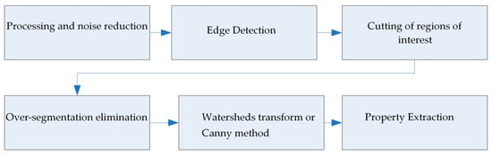
Figure 1.
General segmentation process.
In addition to analyzing the different strategies for each of the stages, two segmentation methods were developed, used for the process of each of them [27]. The first was composed by using the Canny method, and the second method used the watershed transform. The difference between the procedures lies in the edge detection method to be used since, in the case of Canny, it is necessary to perform derivative operations to obtain the regions with particles. On the other hand, in the case of the watershed transform, it is necessary to carry out a procedure that eliminates the noise appended to the binary image product of the selected threshold level [28]. There are different types of noise in an image, such as Gaussian, impulsive, frequency, and multiplicative noise [29], which makes reduction difficult.
2.2. Processing and Noise Reduction
It has been experimentally determined that the median filter [30] has a better performance compared to the Gaussian filter and the average filter, mainly due to the elimination of a large part of the noise, in addition to preserving the edges of the particles, as seen in Figure 2.
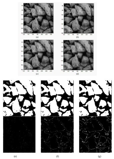
Figure 2.
(a) Original image; (b) application of 3 × 3 median filter; (c) application of 9 × 9 Gaussian filter with σ = 1; (d) application of 9 × 9 average filter; (e–g) binarized images (using Otssu algorithm) and contour by subtraction of original image.
In Figure 2b, the median filter is applied, using the original image, shown in Figure 2a, as the input image, observing that the edges of the structures are not preserved (Figure 2e). The Gaussian filter is used in Figure 2c, where the blurring of the particles is combined with the surrounding regions, determining the possible edges of particles (Figure 2e). Finally, in Figure 2d, the application of the average filter (9 × 9 window) depicts clear borders. The Figure 2e–g are binarized images (using Otssu algorithm) from Figure 2a–c respectively.
2.3. Edge Detection
2.3.1. Sobel Operator
The Sobel operator is a discrete differential that calculates an approximation to the gradient of the intensity function of an image. As it can be seen in Figure 3b, applying the Sobel operator to Figure 3a is not sufficient for edge detection. While it denotes easily visible edges more vividly, it also shows edges that are the result of noise, drift, and the irregular shape of the image. With the help of the minimum elimination operation together with the Sobel function, it is possible to eliminate areas where hypothetical particles will not be found.
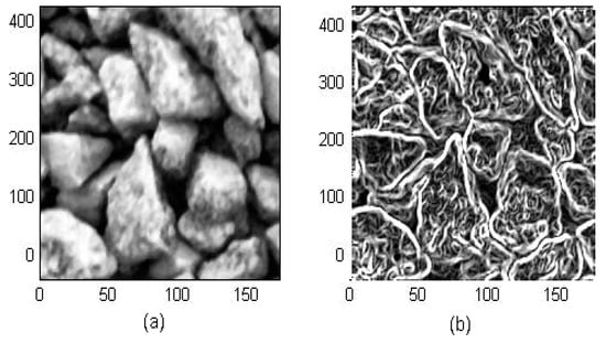
Figure 3.
(a) Original image; (b) application of the Sobel operator in (a).
2.3.2. Canny Operator
The Canny method more accurately detects the edges of structures because it is less sensitive to noise since it uses a Gaussian filter to reduce it. However, it generates many open edges, which is why it is necessary to carry out the dilation, filling, and erosion process. Before applying the Canny operator on the image, unnecessary areas were eliminated by multiplying the binarization of the original image. With the discretized image of Figure 4a and with the 16 discrete values shown in Figure 4b, the result is Figure 4c, which allows the Canny operator to help find the edges of the particles. This results in Figure 4d, where an improvement in the detection of the edges is appreciated, in comparison to the Gaussian filter and Otssu binarization (Figure 2g), as well as a decrease in false edges or those introduced by noise.
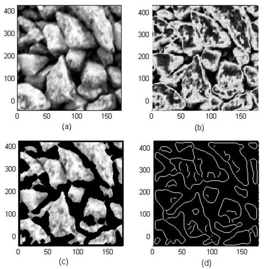
Figure 4.
(a) Original image; (b) discretized image; (c) cropped image; (d) Canny application.
2.4. Cutting of Regions
Once the binarization and the detection of the edges have been obtained, the regions of interest are generated, in which it is possible to find hypothetical particles. To do this, the original binarized image shown in Figure 5a was smoothed, using the opening and closing morphological operators, generating smoother edges, as seen in Figure 5b. This operation tends to increase the internal details of the threshold regions.
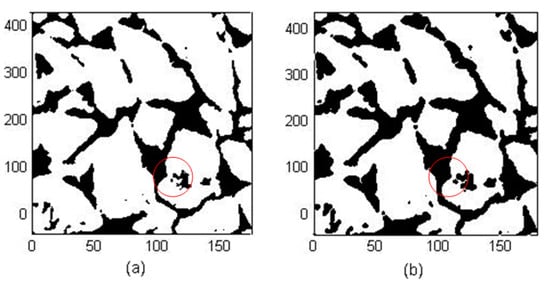
Figure 5.
(a) Binary image; (b) smoothed binary image.
As it can be appreciated in the red circles in Figure 5, the internal details are exalted for a better fit with the edges. Subsequently, this image was eroded, and the gaps were filled (Figure 6a), in order to then expand the edges generated by Canny (Figure 4d) and subtract them from this image, generating regions in which it is possible to find the hypothetical particles, as shown in Figure 6b.
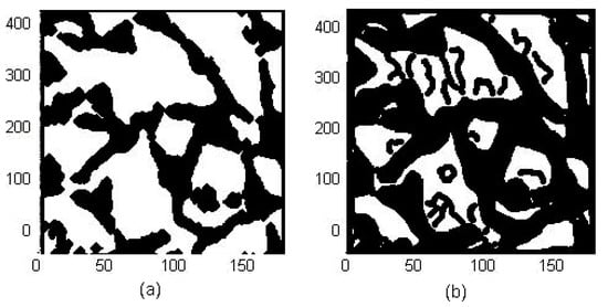
Figure 6.
(a) Filled and eroded image; (b) binary image subtraction and Canny’s dilated edge.
2.5. Elimination of Over-Segmentation
Gray scale images can be transformed into 3D space. In this type of image, each pixel is transformed into a 3D shape using its coordinate (x, y) as the position and its gray level as the elevation. The 3D representation applied to the original image (Figure 4a) with a gray level between 0 and 255 can be seen in Figure 7. The areas that represent peaks are the regions where the hypothetical particles can be found, and the valleys or low areas are regions where there is no interest for the meeting of particles. This interpretation can be used to eliminate over-segmentation, since, as seen in the peaks, there are also valleys, but they are clearly areas where it is possible to find a particle.
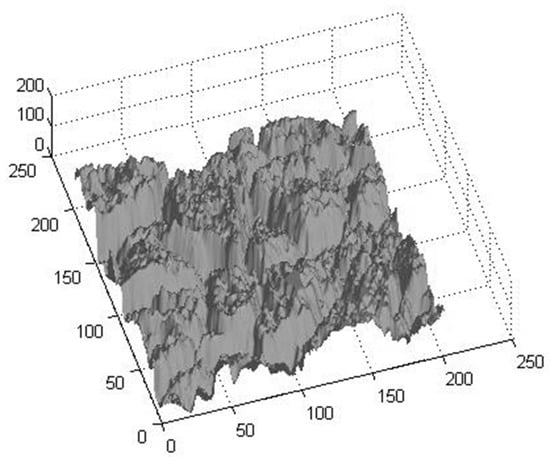
Figure 7.
3D representation of an image.
An image contains multiple local minimum or maximum regions, but only one global minimum and maximum. These maximum and minimum values are used for a morphological reconstruction, segmenting the image through the watershed transform.
To find these minima, the edges found by Sobel (Figure 8a, from Figure 3b) were used, and the image segmented by Canny (Figure 6b) was used as a mask, resulting in Figure 8b.
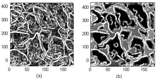
Figure 8.
(a) Sobel image; (b) image generated by “imimposemin”.
2.6. Watershed Transform
After applying the edge detection and over-segmentation elimination methods, with the search for minima, the watershed transform was applied. To improve the performance of the found regions, one of the advantages of this transform is that it only segments the regions based on the images generated by the previous processes.
The watershed transform generates regions which are the limits or edges of the “floods” that it affects. A clear example can be seen in Figure 9b, where the transform is applied to Figure 9a, from Figure 8b.
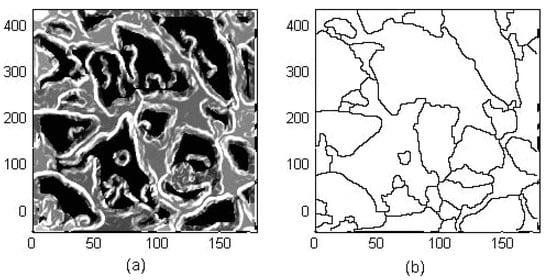
Figure 9.
(a) Gradient image; (b) watershed transform.
As it can be seen in Figure 9b, there is already a first approximation of hypothetical particles. However, it is still necessary to determine, in a better way, the shapes of the regions. For this purpose, the resulting image was complemented (Figure 9b), and the previous segmented image was subtracted (Figure 6a), generating new regions with a closer approximation to the hypothetical particles to be characterized, as shown in Figure 10b.
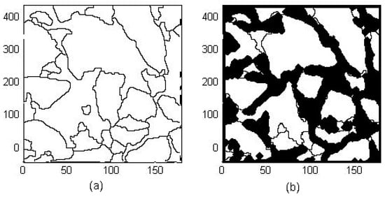
Figure 10.
(a) Watershed result; (b) subtraction result.
In order to further refine the segmentation process, the watershed transform was applied to the maxima found in the image resulting from the subtraction (Figure 10b), in order to know, with a wide margin, the probable regions where a possible hypothetical particle can be found, as seen in Figure 11.
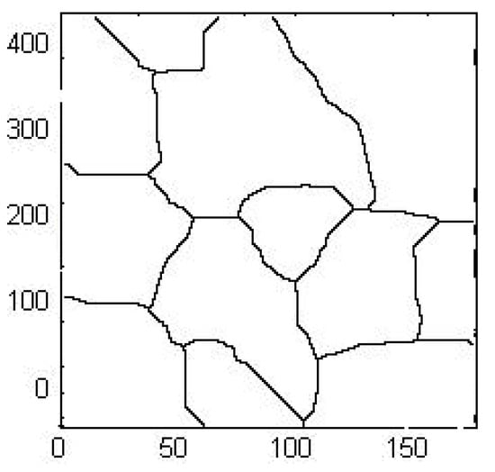
Figure 11.
Watershed segmentation to establish regions of possible particles.
The resulting segmentation was multiplied with the previous resulting image (Figure 10b), and the final segmentation was generated to process and extract the characteristic properties (Figure 12a), coloring them for better identification (Figure 12b).
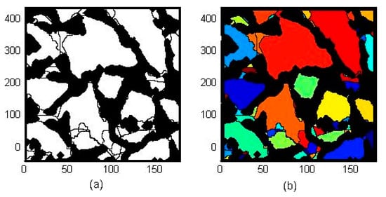
Figure 12.
(a) Final segmentation result; (b) colorized image for better detail.
2.7. Property Extraction
Once each of the hypothetical particle regions was segmented and extracted, we proceeded to extract the characteristic properties of each of these regions. To do this, the “region props” function was used, which was implemented in the Matlab image analysis “Toolbox”. Each of these characteristics returns one or more values that correspond to the measurements carried out, providing the pixels as a reference. In addition, each of these measurements is multiplied by a conversion factor which indicates the measurement to be calculated by the number of pixels.
2.8. Comparison Strategy
A quite complex problem when proposing algorithms that perform image processing is to have a quantitative measurement of their performance, not only in terms of processing time, which can be a relevant factor, but also in terms of the quality of the processing.
In addition, segregation occurs while particles are transported, as a consequence of the conveyor belt vibrations. This phenomenon is well known from plant experience, and it has recently been modeled and studied [31]. This particle segregation settles down small particle sizes, while larger particles emerge to the surface of the bed, as shown in Figure 13. This bias in the sampling procedure (2D imaging) oversamples large particles. This bias allows a better characterization of larger particles, which is the main objective of the technology, in order to detect classification failures (screening) and to reduce subsequent operational problems downstream due to particle plunging in the secondary or tertiary crushing stage.
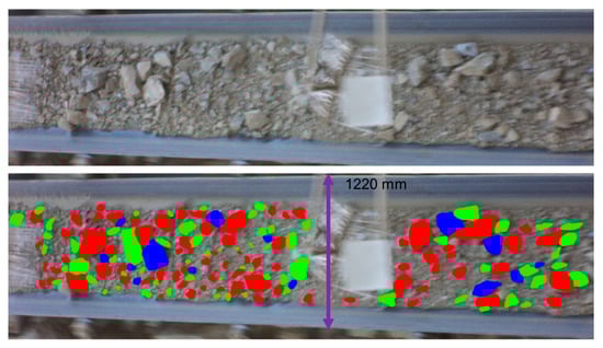
Figure 13.
Manual marking on a conveyor belt (the width of the conveyor belt is represented in blue arrow).
The problem validation is, fundamentally, in having something to compare the performance with, that is, an ideal of the treated image, since, as shown many times, that does not exist unless a person conducts it manually, for example, marking with a specific color in the case of touching objects, as shown in Figure 13.
Figure 13 represents the conveyor belt in operation. To evaluate the performance achieved by the segmentation, it is measured by classifying 2 classes of tests that help measure the performance of the system [30]. These classes are constituted by the set of segmented regions with defects, and those free of defects or that are regular; for this, the “sensitivity” and “1-specificity” tests must be determined.
For each of the comparison cases, it is expected to obtain the following:
- FP: False positives. The number of points where a particle was found but it should not have been.
- FN: False negatives. The number of points where a particle was not found but it should have been.
- VP: True positives. The number of points in successful particles.
- VN: True negatives. The number of points that are not part of a particle but are correctly detected.
These four parameters were used to conduct the sensitivity test, where its equation is:
Additionally, for the “1-specificity” test, the representative equation is:
The first of the Sn indicators takes the value 1 in the case of recognition of all particle points, and 0 in the case of not recognizing any particle points. This indicator shows if the particles that are being searched were found or not, that is, it provides a measure for the sensitivity of the algorithm that is being measured to the test case that is being applied.
The indicator 1 − Sp takes the value 0 in the case of a perfect recognition of the edge points, varying up to 1 in the case of detecting any false positives correctly. Unlike the first indicator, this shows the relative number of points that failed to be detected as edge points, that is, it shows the precision of an algorithm in the test case that it is measuring.
This way of comparing can be questioned since, as shown many times, an algorithm, in general, tends to partially fail, or, sometimes, it is not totally successful but works badly in parts. In any case, this way of comparing is a practical and repeatable technique.
Figure 14 presents an example of the comparison method used to calculate the variables VP, VN, FP, and FN. In this way, the “sensitivity” and “1-specificity” can be calculated when the values of each pixel of the two images are analyzed, and the comparison can be conducted.
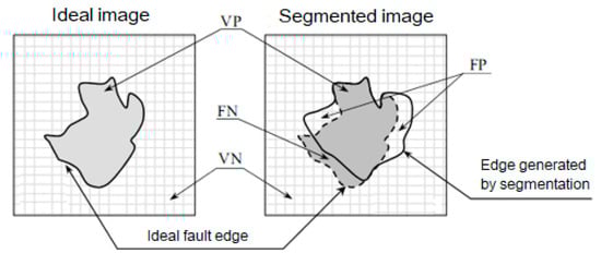
Figure 14.
Representation of the differences between ideal and segmented images.
2.9. Industrial testing
During the commercial validation period, an ANALITA sample prototype was installed to analyze the material carried by the conveyor belt E-135 of the secondary and tertiary crushing plant. This belt is the intermediate point between the 2 crushers; therefore, it is an important point of reference on the size and quality of the transported material.
It is worth mentioning that the tests were conducted with an old USB 1.0 data communication standard, which does not provide all the features that its successors bring. However, for test analysis, it is sufficient to see the behavior of the sensor in industrial sites.
Around 215 samples of photographic images were taken for a period of 30 min, which provided an average material of 300 tons, as seen in Figure 15, which were analyzed and compared with the curves of the percentage passing by weight of such belt.
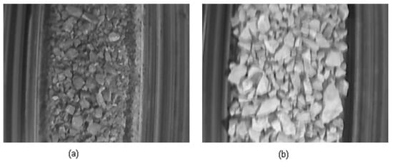
Figure 15.
Sample belt images. (a) and (b) represent different image samples of the total of 215.
The revision of the tests carried out made it possible to formulate the observations detailed in the following points.
2.10. Global Observations of the Test
The tests were compared against the results of historical samples, since, due to the very nature of the mining operation, it was not possible to obtain a real contrast of the same analyzed material (counter-sample).
It should be mentioned that the test methods differ in the way of obtaining the different classes of material, mainly because of the sampling method with Tyler meshes. Although they classify the material according to a diameter established by each type of mesh, its representation of the passing percentage is based on the total weight of the particles, retained by said mesh, contrary to how the classification is conducted by means of image analysis, since this is carried out with respect to the amount that is retained by a certain limit, with the number of total particles. For reasons of the density of the material under study, the results obtained vary according to the margins of this.
To determine the distributions, 2 different classification methods were carried out. First, the characteristic size that defines the ISO standard for granulometric sizes was taken as a reference, and the passing percentages were counted according to the amount under that size with respect to the total amount of particles. For the second method, the percentiles were counted, and the corresponding sizes were derived.
The tests were carried out together with the same conveyor belt, without extracting data from the control room or other PLC (programmable logic controller) control equipment.
3. Results and Discussions
3.1. Rosin Rammler Model Fitting
From a sequence of images collected from the conveyor belt (Figure 15), particles were detected based on the algorithm proposed in this communication. The detection accuracy is 60–67%, as described and analyzed in Section 3.3. Geometrical properties were determined for each detected particle, and size classification for the maximum length was performed based on the geometric progression (Tyler mesh), with a size between 2000 and 100,000 microns. The particle size distribution was obtained by adjusting a mathematical model representing the phenomenology of the crushing process. The Rosin Rammler distribution model is the most accurate model for comminution processes in the case of large particle sizes (crushers). The model was adjusted by applying minimum least squares to the residual (model and maximum particle length frequency). The results for two types of crushing stages (shown in Figure 15) are plotted in Figure 16.
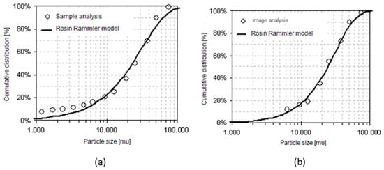
Figure 16.
(a) Granulometric curves of samples. (b) Sensor curve. For images shown in Figure 15.
From this plot, the precision of the adjusted model shows that particle detection and classification correspond to a phenomenon of particle comminution. The mean adjusting error in Figure 16a is 1.6%, while in Figure 16b, it is 4.8%. The deviation in the range of small particles, under 6000 microns, is a consequence of the limited detection capability for 6.35 mm particles. The lower detection capability can be fixed by increasing the camera resolution. However, the main objective of this technology is to detect large particles sizes, not the whole distribution. In this case, for large particles, the error of model fitting is lower and suitable for application in troubleshooting detection.
3.2. Statistical Analysis
As it can be seen in Table 1, the correlation analysis of Analita vs. the sample average reaches a correlation of 99.71% within the 100% and 20% range, which shows a very good precision in size determinations within that range.

Table 1.
Correlation between % passing weight and % passing amount.
To verify the reliability of the correlations, an analysis of variance was performed to determine if there are differential effects between the Tyler mesh method and Analita image analysis. It can be seen in Table 2 that the value obtained for the F statistic is less than its critical error value (0.08 < 4.07), which shows that Analita is a valid method to determine the distribution of granulometric size particles.
Table 2.
Analysis of variance.
3.3. Performance Testing and Comparison
The class classification strategy [32] was used to measure sensor performance. For this, a set of images of particles prepared and taken in the laboratory was used (samples 1 to 6). These were previously segmented and processed through Analita. Then, both were compared, calculating each of the classification values, resulting in Table 3.
Table 3.
Performance analysis in sensitivity and accuracy.
On average, “Analita” has a detection sensitivity (accuracy) to particles of 60% in any image, meaning it will be able to recognize an average of 60% of the particles. Additionally, it has a maximum of almost 67%. Furthermore, the degree of precision of model fitting, on average, is 4.6%, being in a better case 2%, as seen in sample 2.
These results are favorable for the algorithm since they allow the size of the particles to be properly established. It is worth mentioning that sample 6 is an image produced on a computer. When comparing this image, a worse result is appreciated compared to the one taken from the camera, where it only reaches a sensitivity of 38.7%, but instead, it has a perfect recognition of those particles, achieving a precision of 0% (perfect fit) due to no false positive spots emerging.
With these data, it can be demonstrated that the system is capable of segmenting and analyzing 60% of the particles captured by the images.
4. Conclusions and Future Remarks
A hardware and software system for online measurement of particle size distribution based on image analysis was developed and implemented. This analyzer was created by separating the process into stages, such as image acquisition and enhancement, noise reduction and processing, edge detection, region cutting, over-segmentation elimination, watershed transform application, and property characterization, which were finally used to create the size distribution. The prototype and software demonstrated the technical feasibility of using this system in industry. Tests were carried out that showed that the sensor manages to be a suitable tool for particle size analysis.
With the comparison and performance strategy procedure, it was obtained as a result that the sensitivity, that is, the average amount of particles that the analyzer manages to detect in an image, is 60% of the particle area, and the precision (model fitting) is 5%. The analyzer was validated at a mining company of Chile, where an average error of 4.78% was obtained when the Rosin Rambler model was adjusted. Nevertheless, with the Rosin Rammler modeling method, this error was reduced to 1.61% for a coarse material; therefore, this device can be used to determine size distributions on conveyor belts. In addition to this, the most appropriate algorithms could be established to reduce noise, improve the contour of the particles, and optimize the segmentation time through Matlab software.
This system also presents an opportunity for the use of machine learning or deep learning, which would substantially improve its performance and would have the advantage of not needing such repeated adjustments.
Author Contributions
D.C. was responsible for the data collected and the data cleaning. D.C. and C.A. were responsible for the selection and the validation of parameters used on the model’s generation, D.C. and C.L. was responsible for the pre-processing and the validation and interpretation of results. All authors contributed to the design of the experimental design and writing and reviewing the final manuscript All authors have read and agreed to the published version of the manuscript.
Funding
This research received no external funding.
Data Availability Statement
All raw data remain the property of the university that allowed this study. The input data used to support the findings of this study are available from the correspondent author’s email with appropriate justification.
Acknowledgments
The authors thank the Universidad Católica del Norte and 2030 Project for the material support provided and their collaboration with this study.
Conflicts of Interest
The authors declare no conflict of interest.
References
- Newman, T.S.; Jain, A.K. A survey of automated visual inspection. Comput. Vis. Image Underst. 1995, 61, 231–262. [Google Scholar] [CrossRef]
- Gonzalez, R.C.; Woods, R.E. Representation and description. In Digital Image Processing, 2nd ed.; Addison Wesley: Boston, MA, USA, 1992; Volume 2, pp. 643–692. [Google Scholar]
- Li, Y.; Liao, T.W. Weld defect detection based on Gaussian curve. In Proceedings of the 28th Southeastern Symposium on System Theory (SSST ‘96), Baton Rouge, LA, USA, 31 March–2 April 1996; pp. 227–231. [Google Scholar]
- Liao, T.W.; Li, Y. An automated radiographic NDT system for weld inspection: Part II–Flaw detection. NDT E Int. 1998, 31, 183–192. [Google Scholar] [CrossRef]
- Liao, T.W. Classification of welding flaw types with fuzzy expert systems. Expert Syst. Appl. 2003, 25, 101–111. [Google Scholar] [CrossRef]
- Mery, D. Inspección Visual Automática. In Proceedings of the Primer Congreso Internacional de Ingeniería Mecatrónica, Lima, Peru, 8–12 April 2002. [Google Scholar]
- Mery, D.; da Silva, R.R.; Calôba, L.P.; Rebello, J.M. Pattern recognition in the automatic inspection of aluminium castings. Insight-Non-Destr. Test. Cond. Monit. 2003, 45, 475–483. [Google Scholar] [CrossRef]
- Mery, D.; Pedreschi, F. Segmentation of colour food images using a robust algorithm. J. Food Eng. 2005, 66, 358. [Google Scholar] [CrossRef]
- Soille, P.; Vincent, L. Determining Watershed in Digital Pictures via Flooding Simulation. In Proceedings of the Visual Communications and Image Processing (SPIE), Lausavre, Switzerland, 1 September 1990; Volume 1360, pp. 240–250. [Google Scholar]
- Canny, J. Finding Edges and Lines in Images. Master’s Thesis, Massachusetts Institute of Technology (MIT), Cambridge, MA, USA, 1983. Available online: https://dspace.mit.edu/handle/1721.1/6939 (accessed on 25 March 2021).
- Canny, J. A Computational Approach to Edge Detection. IEEE Trans. Pattern Anal. Mach. Intell. 1986, 6, 679–698. [Google Scholar] [CrossRef]
- Heath, M.D. A Robust Visual Method for Assessing the Relative Performance of Edge Detection Algorithms. Master’s Thesis, University of South Florida, Tampa, FL, USA, December 1996. [Google Scholar]
- Breu, H.; Gil, J.; Kirkpatrick, D.; Werman, M. Linear Time Euclidean Distance Transform Algorithms. IEEE Trans. Pattern Anal. Mach. Intell. 1995, 17, 529–533. [Google Scholar] [CrossRef]
- Beucher, S.; Lantuéjoul, C. Use of Watersheds in Contour Detection. In Proceedings of the International Workshop Image Processing, Trieste, Italy, 4–8 June 1979; pp. 17–21. [Google Scholar]
- Beucher, S. The Wathershed Transformation applied to Image Segmentation. In Proceedings of the 10th Pfefferkorn Conference on Signal and Image Processing in Microscopy and Microanalysis, Cambridge, UK, 16–19 September 1991. [Google Scholar]
- Vincent, L. Morphological Grayscale Reconstruction in Image Analysis: Applications and Efficient Algorithms. IEEE Trans. Image Process. 1993, 2, 176–201. [Google Scholar] [CrossRef] [PubMed]
- Meijster, A.; Roerdink, J.B.T.M. The Implementation of a Parallel Watershed Algorithm; University of Groningen: Utrecht, The Netherlands, 1995; pp. 134–142. [Google Scholar]
- Meijster, A.; Roerdink, J.B.T.M. A Disjoint set Algorithm for the Watershed Transform. In Proceedings of the 9th European Signal Processing Conference, Rhodes, Greece, 8–11 September 1998; Volume 3, pp. 1665–1668. [Google Scholar]
- Sang, P.H.; Beom, R.J. Homogeneous Region Merging Approach for Image Segmentation Preserving Semantic Object Contours. In Proceedings of the International Workshop on Very Low Bitrate Video Coding, Urbana, IL, USA, 8–9 October 1998. [Google Scholar]
- Roerdink, J.B.T.M.; Meijster, A. The Watershed Transform: Definitions, Algorithms and Parallelization Strategies. Fundam. Inform. 2001, 41, 187–228. [Google Scholar] [CrossRef]
- Meyer, F.; Vachier, C. Image Segmentation Based on Viscous Floodinf Simulation. In Mathematical Morphology: Proceedings of the VIth International Symposium, Bordeaux, France, 28–30 August 2013; Hugues, T., Richard, B., Eds.; CSIRO Publishing: Clayton South, Australia, 2002; pp. 69–77. [Google Scholar]
- Horowitz, S.L.; Pavlidis, T. Picture Segmentation by a tree traversal algorithm. J. ACM 1976, 23, 368–388. [Google Scholar] [CrossRef]
- Lawson, S.W.; Parker, G.A. Intelligent segmentation of industrial radiographic images using neural networks. In Machine Vision Applications, Architectures, and Systems Integration III; International Society for Optics and Photonics: Bellingham, WA, USA, 1994; Volume 2347, pp. 245–255. [Google Scholar]
- Vincent, L.; Soille, P. Watersheds in digital spaces: An efficient algorithm based on immersion simulations. IEEE Comput. Archit. Lett. 1991, 13, 583–598. [Google Scholar] [CrossRef]
- Rasheed, F.; Dominguez-Ontiveros, E.E.; Weinmeister, J.R.; Barbier, C.N. Deep Learning for Intelligent Bubble Size Detection in the Spallation Neutron Source Visual Target. In ASME International Mechanical Engineering Congress and Exposition; American Society of Mechanical Engineers: New York, NY, USA, 2020; Volume 84584, p. V010T10A001. [Google Scholar] [CrossRef]
- Galata, D.; Mészáros, L.; Kállai-Szabó, N.; Szabó, E.; Pataki, H.; Marosi, G.; Nagy, Z. Applications of machine vision in pharmaceutical technology: A review. Eur. J. Pharm. Sci. 2021, 159, 105717. [Google Scholar] [CrossRef] [PubMed]
- Mery, D.; Filbert, D. Automated Flaw Detection in Aluminum Castings Based on the Tracking of Potential Defects in a Radioscopic Image Sequence. IEEE Trans. Robot. Autom. 2002, 1, 890–901. [Google Scholar] [CrossRef]
- Pichel, J.C. Algoritmo Paralelo de Segmentación Basado en Agrupamiento de Regiones en Imágenes Sobre-Segmentadas. Bachelor’s Thesis, Universidad de Santiago de Compostela, Departamento de Electrónica e Computación, La Coruña, Spain, 2002. [Google Scholar]
- De la Escalera, H.A. Visión por Computador, fundamentos y métodos; Prentice Hall: Madrid, Spain, 2001. [Google Scholar]
- Castleman, K.R. Digital Image Processing; Prentice Hall: Hoboken, NJ, USA, 1996. [Google Scholar]
- Gajjar, P.; Johanson, C.; Carr, J.; Chrispeels, K.; Gray, J.M.N.T.; Withers, P. Size segregation of irregular granular materials captured by time-resolved 3D imaging. Sci. Rep. 2021, 11, 8352. [Google Scholar] [CrossRef] [PubMed]
- Egan, J.P. Signal Detection Theory and ROC Analysis; Academic Press: Cambridge, MA, USA, 1975. [Google Scholar]


Publisher’s Note: MDPI stays neutral with regard to jurisdictional claims in published maps and institutional affiliations. |
© 2021 by the authors. Licensee MDPI, Basel, Switzerland. This article is an open access article distributed under the terms and conditions of the Creative Commons Attribution (CC BY) license (https://creativecommons.org/licenses/by/4.0/).