Analysis of Mining-Induced Delayed Surface Subsidence

Abstract

The topic of residual subsidence is important in Europe as it defines possible surface deformation for closed mine areas. It has to be determined because of potential financial claims and damages of sensitive objects such as satellite dishes, precision mechanics objects, agriculture, forestry and hydrogeology, etc. Analyses of measured subsidence after the end of mining exploitation indicate that this process can last from several months to several dozen or even several hundred years, and the final surface subsidence is not known. It is dependent on the individual’s features of excavated medium, depth of exploitation, a system of exploitation, behaviour of surrounding rock masses, etc. In the article, the authors analysed the assessment of the subsidence process after the end of mining operations, based on the innovative method. This concerns the duration of the subsidence process and the size of the expected subsidence. The methodology was applied to the RAG Aktiengesellschaft company project where prognostic calculations were made for seven closed coal mines using unique results of precise height measurements carried out for more than 90 years by the German State Office for National Measurements (Landesvermessungsamt NRW) under the so-called levelling measurements net. These measurements are carried out every 2 years and serve to keep the altitude network in the whole state of Rhineland Westphalia up-to-date. The result of the prognosis for one case study, German mine Auguste-Victoria, is presented in the article.

1. Introduction

It is an undeniable fact that underground mining operations have degraded the environment over the past decades, despite various attempts to minimise their impact [1,2,3]. From a rock mechanics point of view, the exploitation leads to changes in the original state of stress and deformations in the rock mass [4,5]. One of the most typical forms of such changes is the continuous deformation of the surface, which takes the form of land subsidence. Additionally, it has a significant impact by affecting the reliability of the surrounding land and infrastructure. Over the last century, many methods and theories have been developed to predict mining surface deformations during the extraction of the deposit, i.e., [6,7,8,9,10]. However, these works mainly encompass the problem of deformation during the ongoing mining operation, because at this stage, it has the strongest impact on changing the landscape of the area (terrain and water conditions). In the United States, shallow mining at the depth of ca. 300–400 m below ground level in many places has led to a change in the function of land use [11]. Numerous former pastures have been turned into floodplains as a result of creating large regional subsidence basins and their subsequent flooding. In Europe, due to the location of mining in highly urbanised areas, this problem is mainly related to the occurrence of mining damage to building structures. Usually, this includes damage to residential buildings, outages of transmission networks, and damage to transport facilities (roads, railways), e.g., [12,13].

Contrary to popular belief, the problem of deformation of the rock mass and the ground surface does not end when exploitation ends [14]. At the beginning of the 20th century, there were changes in how the exploitation of deposits was conducted (especially multi-seam exploitation and with roof collapse). The mining moved to greater depths (even more than 1000 m), which over the years led to the formation of hundreds of goafs in the rock mass, i.e., post-mining spaces partially filled with rock material, the compaction of which can be observed long after the mining ends.

The measurements of subsidence usually concern short-term observations of one longwall panel or a set of panels or long-term observations of the entire coal basin. Short-term measurements are usually carried out as part of the ongoing monitoring of the impact of mining on surface infrastructure facilities and typically end between 0.5 and 1 year after the end of a mining operation. The decision to end the observations is based on various criteria, based on many years of experience. In Poland, for example, it was assumed that the impact ceases when the annual increase in subsidence is less than 1.0 cm; in Germany, this is covering its liability for damage which can be reported up to 3 years after the end of the mining operation. In China, this period ends if there is less than 0.3 cm of accumulated surface subsidence during a period of six months, which indicates a stabilised surface movement [6]. The same term was adopted for measurements in Ukraine. In Russia, the last series of measurements are carried out if the subsidence does not exceed 10 mm within 6 months.

Long-term observations of the whole coal basin, covering even several dozen mines, have been carried out to this day in the form of precise levelling for over a hundred years, and in the last period, usually every two years (e.g., Ruhr Basin).

Finding the limit value and the moment at which the impact ceases is important for the assessment of the disturbances in the environment and the provisions of the Mining and Geological Law, which says that at the end of the exploitation, the owner is obliged to restore the land to the state that is as close as possible to its original state, allowing its further use. In the event of successive mine closures [15], the issue of reclamation and revitalisation of land and its costs is important [16]. Depending on the level of degradation, it is possible to give this land a new purpose and utility function, e.g., recreational, agricultural, residential, or commercial. The new opportunities, depending on the application, may become possible for local communities, by acquiring new investments, jobs, the inflow of inhabitants, funds to the budgets of municipalities/cities, or increasing the popularity among tourists. However, for this purpose, it is also important to know about the further impact of mining on the land surface. Based on the results of geodetic measurements of surface subsidence carried out during the operation of the RAG mines and after its closure (31 December 2015), the authors proposed a solution enabling the calculation of residual subsidence of the land surface. This solution makes it possible to determine both the final amount of subsidence and the approximate time at which the deformation value assumed as the limit for residual subsidence is achieved.

2. Experiments with the Determination of Residual Surface Deformations at the End of Underground Exploitation

Initially, it was generally assumed that surface movement caused by underground mining could be divided into two stages: active subsidence and residual or delayed subsidence. The latter is related to the direct exploitation and reaction of the rock mass. They are recorded with a possible delay [17] and represent about 80–90% of the final subsidence level. The former, i.e., residual subsidence, occurs over a long period of time after the end of exploitation. This division was then extended to three stages [18,19]. The stage of active subsidence was divided into the following: preliminary subsidence (phase I), in which from 5% to 15% of final subsidence is observed, and main subsidence (also called accelerated) (phase II), in which from 70% to 90% of final subsidence is observed. Stage III contains the residual subsidence mentioned above (Figure 1), which might range from 1% to 10% of the final subsidence.

It is generally accepted that during the lifespan of a mine, the surface subsidence measurements are carried out up to a maximum of one year after the end of its exploitation, which is also provided in the regulations [20]. This is because a large part of the residual subsidence—from 40% to 80%—appears at the end of the first year [19]. In the following years, the rate of subsidence decreases significantly. It is a brief period in the analysis of residual subsidence, the influence of which may be evident for decades. It is caused by the process of convergence of goafs and the related phase of long-term reconsolidation. Back when the mines existed and operated, the topic of residual subsidence was omitted, which led to a lack of general knowledge in this area. The situation changed along with the process of closing mines. According to Hoek [21] currently, residual subsidence is one of the main problems related to closed mines because the difficulty of determining its duration significantly affects the assessment of environmental degradation and construction problems. The period in which the occurrence of subsidence is possible varies depending on many factors. These include methods of exploitation, backfilling, the intensity of exploitation in the area, the strength of coal, roof and floor, the range and intensity of cracking in the rock mass, rock bulking, the number of water inflows, depth of exploitation, the existence of faults, seam tilt, and speed of exploitation—to list a few. For example, for partial exploitation, such as the room and pillar system, this time depends on the temporary strength of the pillars and can be postponed until the pillar is destroyed and the roof collapses. Examples can be found in works describing this phenomenon, among others: [22,23].

One of the more interesting works on the level and duration of residual subsidence after the closure of a coal mine is the paper by Vervoort and Declercq [24]. Based on subsidence measurements, the authors conducted an extensive analysis of the changes existing at the surface, long after the Houthalen mine was closed in Belgium. In this area, the total thickness of exploited seams ranged from 2.8 to 9.9 m, with the thickness of individual seams ranging from 1 to 2 m. Their tilt varied from 9° to 24°, and the mining took place between the years 1939 and 1968, but most of the longwalls were mined in the years 1940–1960. Observations showed that even 40–60 years after the extraction ended, subsidence still occurs and can be measured. The level of residual subsidence ranged from 2.8 to 8.7 mm/year (5.5 mm/year on average) and reached a maximum of 72.2 mm (average 45.5 mm). This process was disrupted after 2000 when the process of sinking the mine began. It caused both an acceleration and change in the character of how the terrain surface deformed, with the region being partially raised at an average speed of 18 mm/year and partially lowered by 16 mm/year. Similar conclusions as to the duration of residual subsidence were presented, among others by Keinhorst [8] and Niemczyk [25].

Other conclusions from observing the duration of residual subsidence were presented by Flaschentrager [26], suggesting that for the area of the left Lower Rhine, the subsidence process practically ends about six months after the cessation of mining. These results were confirmed by Czubik [27] and Knufinke [28]. The in situ measurements showed that one month after the end of exploitation, about 50% of the expected subsidence took place, after two months 75%, after three 87%, after four 93%, after five 97%, and after six months about 100%.

Blachowski and his team [29], Głowacki, Milczarek [30], Schäfer [31], and Lein [32] drew other conclusions based on satellite measurements (mainly InSAR), from which they determined the duration of surface movements to range from five to a maximum of ten years after the end of exploitation. Similar conclusions were presented in the report from the Bureau of Land Management USDI [33], which concluded that the duration of residual deformations over longwall operations is relatively short and ranges from a few weeks to 10 years. Studies carried out for the mining region of France have shown that during the last two or three years of the residual subsidence phase, the amplitude of subsidence is negligible [19]. In the Nord and Pas-de-Calais area (France), where mining was discontinued in December 1990, the existing measurement points showed different behaviours over time, but all showed an overall decline in subsidence in the years 1992–1999. In fact, from the end of 1992 to 1996, they all subsided by an additional 4 cm in the Courrières area and by 2 cm in Billy-Montigny [19] (the rate of subsidence $S_t$ was 1.25 cm/year on average). On the other hand, no further deformations were observed in the Courrières area after 1996, which shows that the area is stable or that the registered deformation amplitude was below the detection threshold of the DINSar method used (about 0.3 cm/year). On the other hand, both the Lens and Billy-Montigny areas continued to show small movements from 1996 to 1999, while the rates of subsidence S_t were reduced for Lens from 1.2 to 0.7 cm/year and for Billy-Montigny from 0.8 to 0.5 cm/year. The conducted interferograms (Envisat) for the period 2004–2007 confirmed the absence of a significant signal from Courrières, while the Lens and Billy-Montigny regions showed an additional reduction of ca. 0.3 cm per year. In the Marienau region (Lorraine coal basin, France), the total residual subsidence is between 20 and 55 cm, and the stabilisation period was less than two years, while the location of the maximum residual subsidence occurs at a distance of 700 m from the location of the maximum level of subsidence related to phases I and II [18]. In this example, the residual subsidence value is equal to 5% of the maximum subsidence value. However, it should be noted that in the presented case, the residual tilt of the land surface is at 0.2% of the maximum value of Tmax, and the total tilt increased from 1.8% (before the residual subsidence phase) to 2% (after the residual subsidence phase) [34], which, in the case of fixed values of the mining area category indexes, may in some cases show that the predetermined category is exceeded [35].

There are similar results of displacement measurements carried out for the city of Bytom (Poland) [36], where multi-seam mining was carried out for years in the safety pillar. In total, the coal mine KWK Centrum exploited the deposit in this area to a total thickness of up to 30 m. In April 2015, the mine ceased its operations, which had lasted (under various names) since the 1950s. The last exploitation in the midtown pillar was carried out in the seam 510 with a longwall system and a hydraulic backfill of a height of 2.4 m. The depth of the exploitation was 650 m with the 140 m front width. In the period from May 2015 to September 2018, the measured subsidence in the area of the last exploitation generally ranged from 2.5 to 27.2 mm. When analysing the last three years after the end of the operation, the annual reduction increments ranged from +2.9 mm (uplift) to −4.2 mm (subsidence). In the last year, the subsidence was between 0.2 and 3.0 mm. These observations led to the conclusion that this area, which was influenced by many years of underground mining, could be considered stable in two years after the mining operations had ended. It is estimated that the subsidence of the mining area after the end of exploitation will still be seen with values of ±1 mm/year. However, they will not affect building structures.

Table 1. Duration and amplitude of residual subsidence phase [18,37].

Cases	Mining Conditions	Residual Subsidence
UK (Many basins)	Long-wall method and plastic layers	Less than 12 months: 5–6% of total subsidence
UK (Durham Coalfield)	Two mines with high-resistance strata	8% of total subsidence after 4 years and 9% after 6 years, and 6–8% of total subsidence after 4 years
West Germany	Long-wall method used by many mines	5 years with 75% from the first year
Australia	Long-wall with caving method	3 to 7 months
India	Long-wall method in virgin ground	10–15 months for 10–30% of total subsidence
	Long-wall method in already extracted zones	2–4 months for 5–10% of total subsidence
USA	Long-wall method	10% of total subsidence: 1 month and 12% after 17 months
France (Nord-Pas-de-Calais, Albi-Carmaux)	Plastic strata in already extracted zones	99% of total subsidence after 3–4 years
France (Provence, Lorraine, and Blanzy)	Resistant strata in already extracted zones	2–3 years

shows additional data on the duration and amplitude of phase III related to residual subsidence.

3. Methods of Forecasting the Residual Subsidence Value after Exploitation Ends

As shown in the above experiences of worldwide scientists, discrepancies in the duration of residual subsidence are highly significant. Unfortunately, this problem is often overlooked in the course of mining operations due to its low percentage value compared to deformations originating from phase I or II subsidence, or the problem of determining residual deformations with overlapping (superposition principle) influences from progressive mining. In turn, after the mines are closed, this problem is often neglected by local government authorities, such as the situation in South Korea presented by Lee [38]. It is therefore important to have the appropriate tools to predict future residual subsidence.

Several scientists from all over the world have dealt with the topic of residual subsidence forecasts in their work. One of the earliest was Professor Knothe [39], who in the 1950s presented a solution for determining the time function z(t) in the form:

$$\begin{gathered} \dot{s}\left(t\right)=c\left[s_k\left(t\right)-s\left(t\right)\right] \\ z\left(t\right)=1-exp\left(-ct\right), \end{gathered}$$

(1)

where $\dot{s}\left(t\right)$ is the momentary speed of subsidence, $c$ is the time factor, $s_k\left(t\right)$ is the final subsidence of the point with the assumption of the exploitation end in time t, $s\left(t\right)$ is the real value of subsidence, $z\left(t\right)$ is the function of time, and $t$ is time.

In the following years, similar work was carried out by Trojanowski [40]. A two-parameter model of the time function was presented by Schober and Sroka [41] describing the process of subsidence above salt caverns, whereas Sroka’s [42] solution is empirical. In 2013, Liu Xinrong [43] presented a method of forecasting land surface subsidence based on the new time function method, taking account of the dynamic process, the velocity change process, and the acceleration change process during surface subsidence. The use of this solution showed that it predicts values higher than the measured ones and was applied to subsidence with a duration of up to 30 months, i.e., mainly related to phase I and II, rather than to phase III, i.e., residual, long-term subsidence. A similar solution was presented in the article by Hu [44], where authors tried to determine the value of the time factor c of Knothe’s function, which relates only to the active subsidence process [45,46,47].

Cui [48] presented an interesting solution showing the possibility of determining future residual subsidence at the end of the exploitation process. According to the solution presented in the paper, the annual residual subsidence coefficient ($a_A^t$) can be calculated using the equation:

$$a_A^t=k\left(1-a\right)\left(1-e^{-\left(\frac{50-t}{50}\right)}\right)$$

(2)

where a is the surface subsidence factor (ranging from 0.65 to 0.90 in China), k is a coefficient related to the compaction of goaf, which is between 0.5 and 1.0, and t is the time after the end of extraction.

According to Equation (2), for the time span t = 50 years, the annual residual subsidence $a_A^t$ is reduced to 0.

On the other hand, Sroka [45,49] proposed a eaquation to describe the subsidence in time at the end of Exploitation (3):

$$s\left(t>T\right)=s\left(T\right)+\left[s_e\left(T\right)-s\left(T\right)\right]\left[1-exp\left(-c\left(t-T\right)\right)\right]==s_e\left(T\right)-\Delta s_e\left(T\right)·exp\left(-c\left(t-T\right)\right),$$

(3)

where T is the end time of exploitation in the area, s(T) is subsidence in time T, s_e(T) is total final subsidence, Δs_e(T) is the expected increase in subsidence after the end of the time of exploitation in time T, and t is the year for which subsidence is calculated.

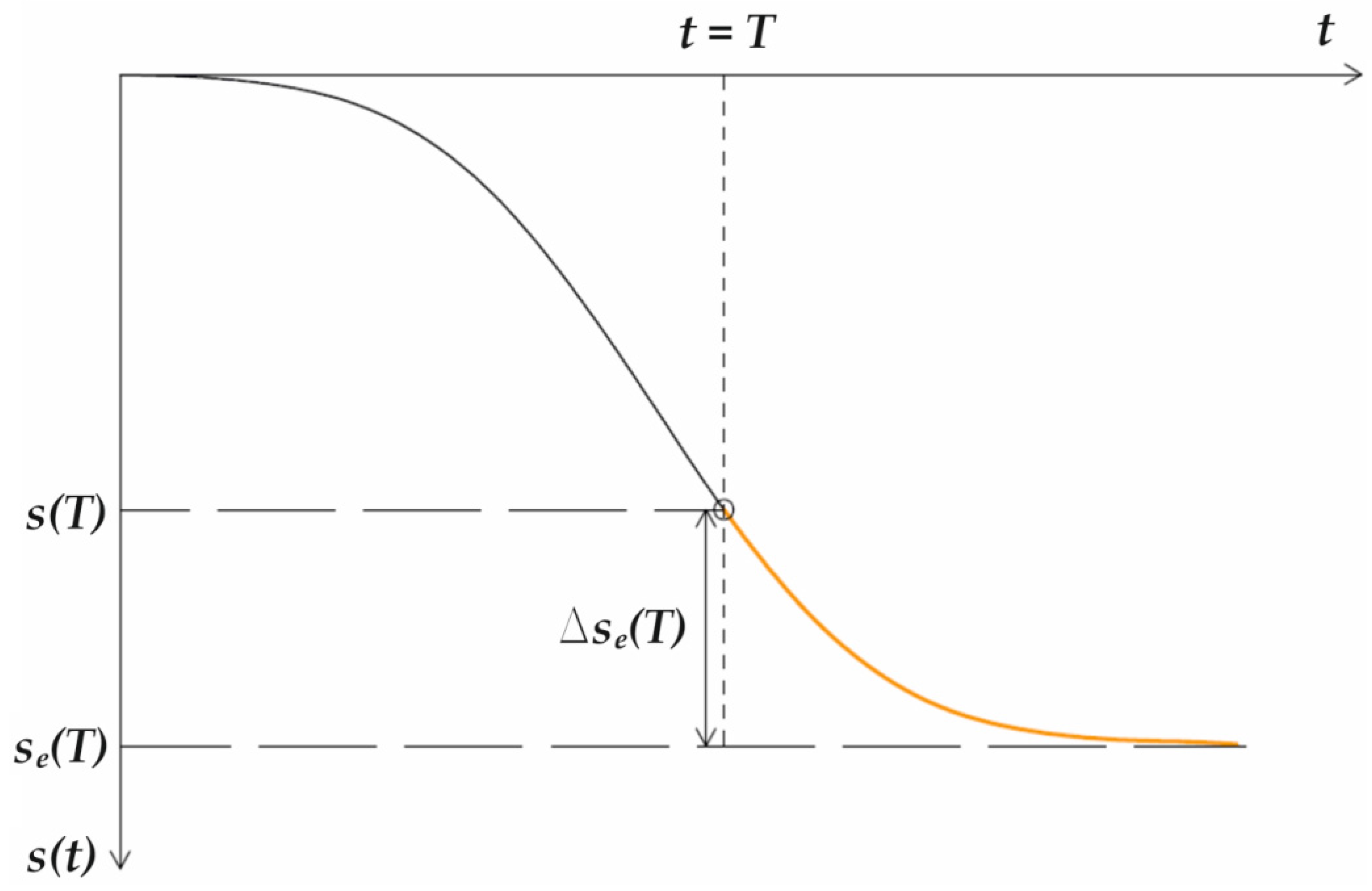
There is a relationship between s(T), s_e(T), and Δs_e(T), which is schematically presented in Figure 2: $s_e\left(T\right)=s\left(T\right)+\Delta s_e\left(T\right).$

4. Methods of Forecasting Residual Subsidence

The observations conducted for the areas of closed underground mines covered by the measurements showed that the subsidence after the end of exploitation is described by means of an exponential, asymptotic function aimed at the expected value of the final subsidence. These observations, together with analyses of the recorded displacements during exploitation, made it possible to develop a three- or four-point solution enabling one to forecast future values of final residual subsidence and determine the time span to achieve the limit value of residual subsidence ∆s_Gr, i.e., the level of subsidence significant for the future use of the land (Figure 5) [50]. The three- or four-point solution is selected depending on the length of the measurement period, the number of measurement points that can be used, and the course of exploitation.

For the three-point solution, the same interval between measurements is assumed, i.e., $t_3-t_2=t_2-t_1=\Delta t$. The subsidence diagram for the three-point solution is shown in Figure 3.

The final subsidence in time ($s_e$) can be calculated from equation:

$$s_e=\frac{s_2^2-s_3{s}_1}{2s_2-\left(s_3+s_1\right)}$$

(4)

where $s_1$, $s_2$, and $s_3$ are the individual levels of subsidence for the measured point at equal intervals.

The time factor c is determined by Equation (5):

$$c=-\frac{1}{\Delta t}ln\frac{s_3-s_2}{s_2-s_1}$$

(5)

where Δt is the interval between measurements $t_3-t_2=t_2-t_1$.

For the presented three-point solution, the authors determined the value of standard deviation for subsidence in time with Equation (6):

$$s_{s_e}=\frac{s_s}{2s_2-\left(s_1+s_3\right)}\sqrt{{\left(s_e-s_1\right)}^2+4{\left(s_e-s_2\right)}^2+{\left(s_e-s_3\right)}^2},$$

(6)

where $s_s$ is the accuracy of subsidence measurement (standard deviation), and the value of standard deviation for time factor $c$ is the one in Equation (7):

$$s_c=\frac{s_s}{\Delta t}\sqrt{\frac{1}{{\left(s_2-s_1\right)}^2}+\frac{1}{{\left(s_3-s_2\right)}^2}+\frac{{\left(s_3-s_1\right)}^2}{{\left(s_2-s_1\right)}^2·{\left(s_3-s_2\right)}^2}}$$

(7)

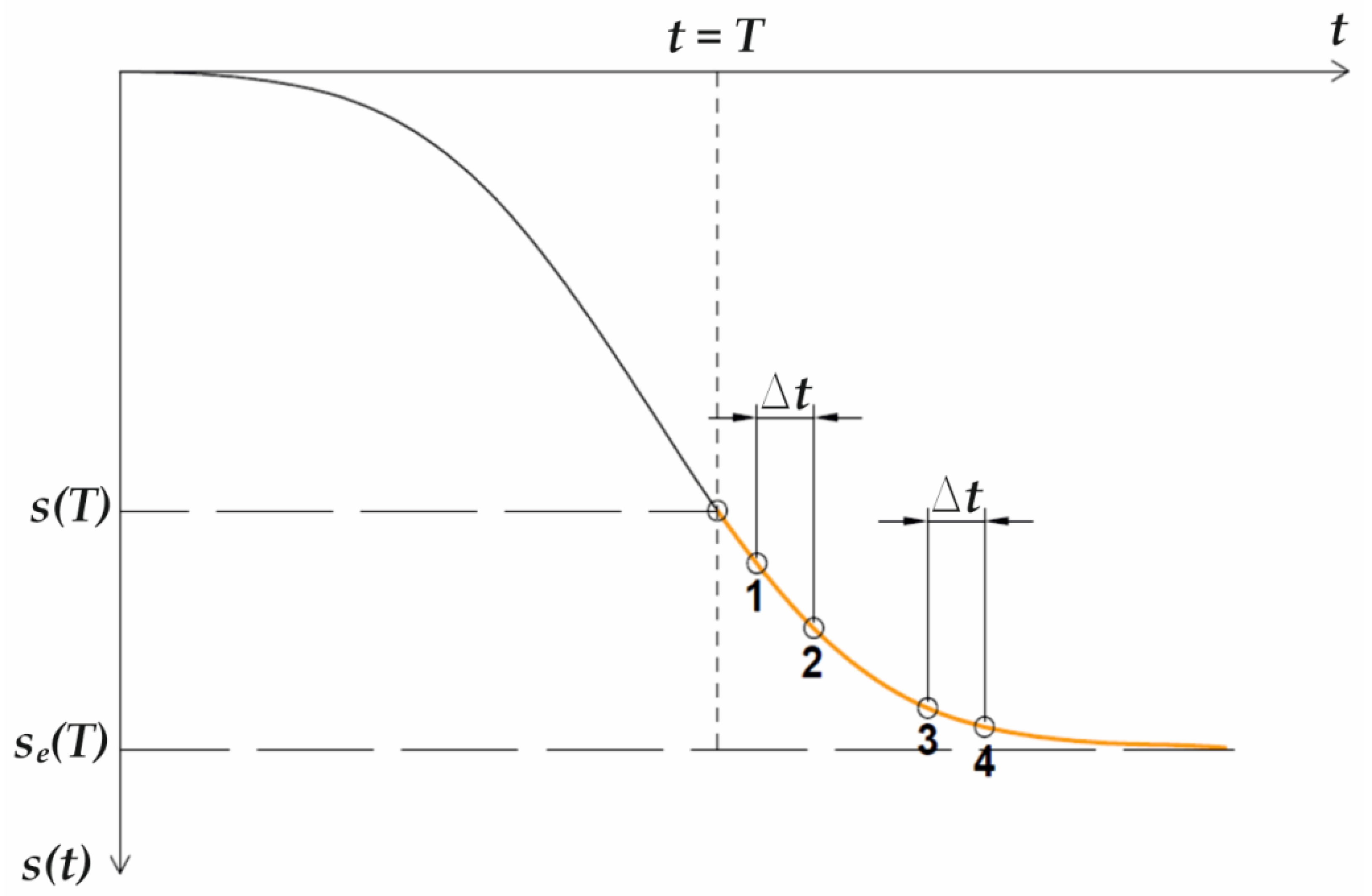
the four-point solution assumes the same interval between measurements, i.e., $t_4-t_3=t_2-t_1=\Delta t$. This situation is illustrated in Figure 4.

In this solution, the following Equation (8) is used to calculate the final subsidence in time ($s_e$):

$$s_e=\frac{s_3{s}_2-s_4{s}_1}{\left(s_3+s_2\right)-\left(s_4+s_1\right)}$$

(8)

However, similarly as in the solution in Equation (5), the time factor for the four-point solution takes the following equation:

$$c=-\frac{1}{\Delta t}ln\frac{s_4-s_2}{s_3-s_1}$$

(9)

The standard deviations of subsidence in time ($s_{s_e}$) as well as the standard deviations for the time factor ($s_c$) are as follows:

$$s_s{}_e=\frac{s_s}{\left(s_3+s_2\right)-\left(s_4+s_1\right)}\sqrt{{\displaystyle \sum }_{i=0}^{i=4}{\left(s_e-s_i\right)}^2}$$

(10)

$$s_c=\frac{s_s}{\Delta t}\sqrt{\frac{2}{{\left(s_3-s_1\right)}^2}+\frac{2}{{\left(s_4-s_2\right)}^2}}$$

(11)

However, it should be noted that measurements are rarely taken when the extraction ceases. According to the presented theoretical solution, the starting point for the description of subsidence after the end of the extraction process can be any measured subsidence in time $t_i>T$. In such a case, a solution describing the course of subsidence in time is used for $t_i<t$:

$$s\left(t>t_i\right)=s\left(t_i\right)+\Delta s_e\left(t_i\right)·\left(1-exp\left[-c\left(t-t_i\right)\right]\right),$$

(12)

where

$$\Delta s_e\left(t_i\right)=s_e-s\left(t_i\right)$$

(13)

as mentioned, the function describing the change in residual subsidence over time is described by an exponential function (Equation (3)), which is asymptotic to the value of the expected final subsidence s_e. This allows us to specify deterministically the expected time span needed for the process of subsidence to end. However, this is closely linked to the definition of mining damage, i.e., the moment at which subsidence ends should be determined in a way that the subsidence that may occur after that moment is insignificant regarding the environment, construction works, or changes in water conditions. This value was used as the limit level (Δs_Gr) for the end of subsidence. Such value should be determined according to the problem, based on existing experience and theoretical considerations.

For example, in agriculture, subsidence affects groundwater levels, which in turn is subject to significant natural fluctuations. According to Knufinke [28], the frequency of precipitation influences the fluctuations of the groundwater level, ranging from 0.5 to 2.0 m during the year. It can increase to 3.0–4.0 m during long periods of drought or rainfall. Studies carried out by Benning [51] in the Etzel area (Germany) showed that groundwater fluctuations reach an average of 1.0 m. This results in a minimum natural groundwater level fluctuation of ca. 0.5 m per year. The assumption that a change in groundwater level associated with residual subsidence of <10% of the natural minimum fluctuation does not have a significant impact on agriculture and forestry leads to a limit value for residual sedimentation $\mathsf{\Delta }{s}_{Gr}$ = 50 mm.

The time when subsidence practically ends is determined by the solution in Equation (12), using Equations (14) and (15):

$$\Delta t_i\left(\Delta s_{Gr}\right)=-\frac{1}{c}ln\frac{\Delta s_{Gr}}{s_e-s\left(t_i\right)},$$

(14)

$$t_e\left(\Delta s_{Gr}\right)=t_i+\Delta t_i\left(\Delta s_{Gr}\right)$$

(15)

where $s\left(t_i\right)$ is the subsidence measured at time $t_i$, and $t_e\left(\Delta s_{Gr}\right)$ is the time needed to achieve the expected (limit) residual subsidence $\Delta s_{Gr}$.

The uncertainty of the time to reach the residual subsidence limit, determined in this way, is described by Equation (16):

$$s_{te}=\frac{1}{c}\sqrt{{\left(\Delta t\left(\Delta s_{Gr}\right)\right)}^2·s_c^2+\frac{s_{s_e}^2+s_s^2}{{\left(s_e-s\left(t_i\right)\right)}^2}}.$$

(16)

The meaning of the symbols is shown in Figure 5.

5. Determination of Final Subsidence and Subsidence Time for the Site of a Former Coal Mine Case Study

The new solutions presented above were used in cooperation with RAG (Germany) to assess future deformations for the area of the former Auguste-Victoria mine, which was closed on 31 December 2015. During the mine’s existence, geodetic measurements of surface displacements were carried out using the precision levelling method with an average accuracy of less than ±2.0 mm, with a standard deviation of 2.8 mm. The first observations were carried out as early as 1921, and from 1990 they were conducted regularly at intervals of two years. The observations were led by the German State Office for National Measurements (Landesvermessungsamt NRW) under the so-called levelling measurements net aimed at keeping the altitude network in the whole state of Rhineland Westphalia up to date. Figure 6 shows the area of the ground surface with outlines of the exploitation and the measurement points stabilised on the surface. For the analysis, the authors of the article adopted 10 measurement points in areas where mining operations were ended in different periods (

Table 2. Dates of cessation of exploitation in the areas of specific measurement points.

Measuring Point Number	Year Exploitation Ended in the Area of the Point
4208900006	2009
4208900008	1989
4208900318	1999
4208900326, 4208900327	2012
4208900331, 4208900362, 4208900366	2015
4208900377	2006
4208900385	2014

).

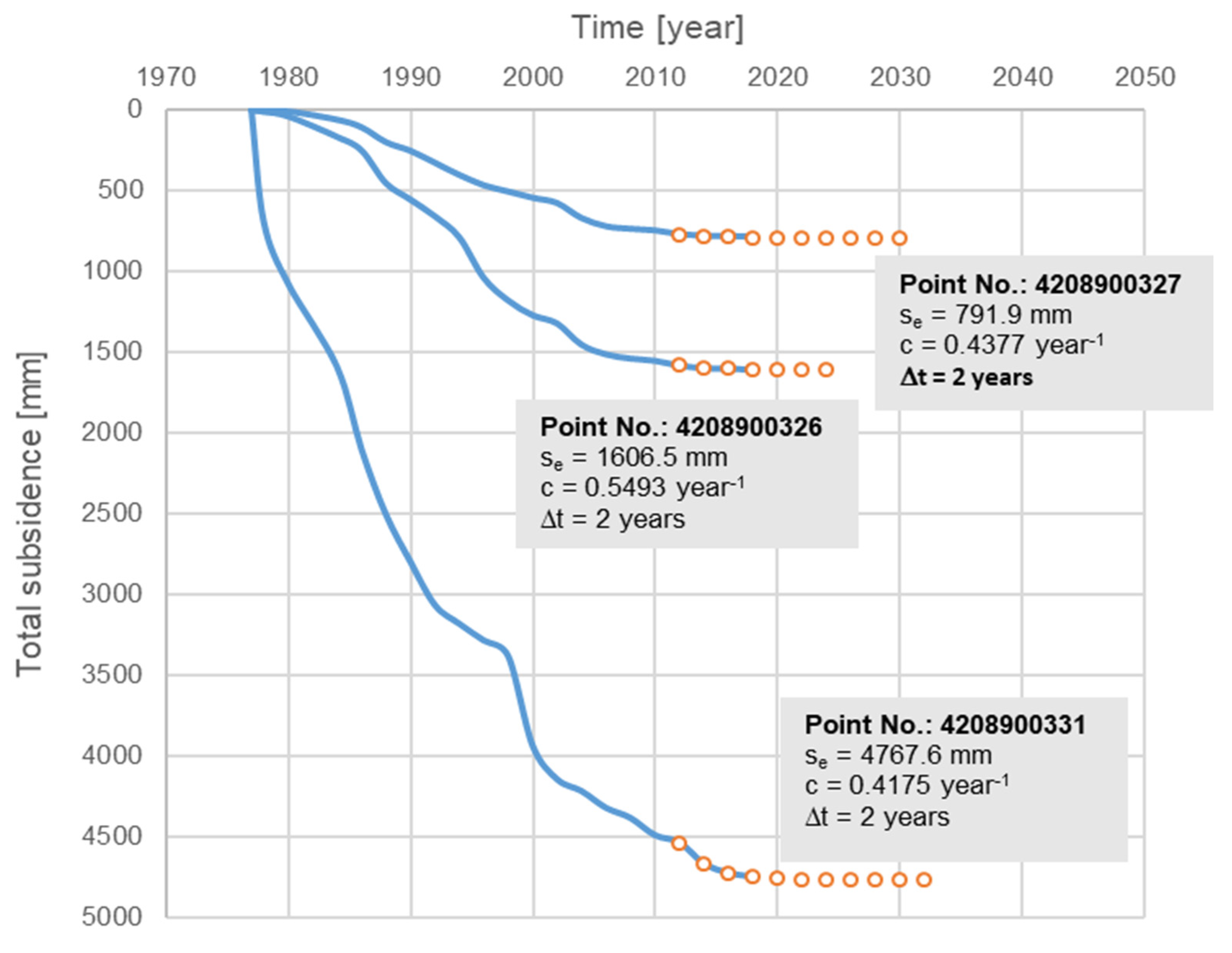
Prognostic calculations of the total final subsidence were carried out, and the time needed for the measuring points to reach the residual subsidence limit was determined. The analyses were based on the solutions presented in the previous chapter using the proprietary method.

Table 3. The values of the measured subsidence of measurement points 4208900006–4208900327 in the individual periods of time from the moment when exploitation ceased in the individual areas.

Year	Subsidence for Individual Measuring Points [mm]
	No. 4208900006	No. 4208900008	No. 4208900318	No. 4208900326	No. 4208900327	No. 4208900331	No. 4208900336	No. 4208900362	No. 4208900377	No. 4208900385
2002	-	795.0	-	-	-	-	-	-	-	-
2004	-	809.0	-	-	-	-	-	-	-	-
2006	-	825.0	266.0	-	-	-	-	-	2378.0	-
2008	2289.0	833.0	277.0	-	-	-	-	-	2422.0	-
2010	2347.0	839.0	284.0	1554.0	750.0	4493.0	-	-	2446.0	-
2012	2383.0	849.0	286.0	1584.0	773.0	4538.0	-	770.0	2467.0	242.0
2014	2435.0	860.0	295.0	1599.0	784.0	4668.0	2015.0	824.0	2489.0	267.0
2016	2454.0	866.0	298.0	1604.0	785.0	4727.0	2128.0	854.0	2503.0	279.0
2018	2464.0	869.0	300.0	1609.0	789.0	4750.0	2156.0	865.0	2511.0	283.0

“-” means that in a given period the point was under the influence of active mining.

shows the values of measured subsidence of measurement points in the last measurement cycles until 2018.

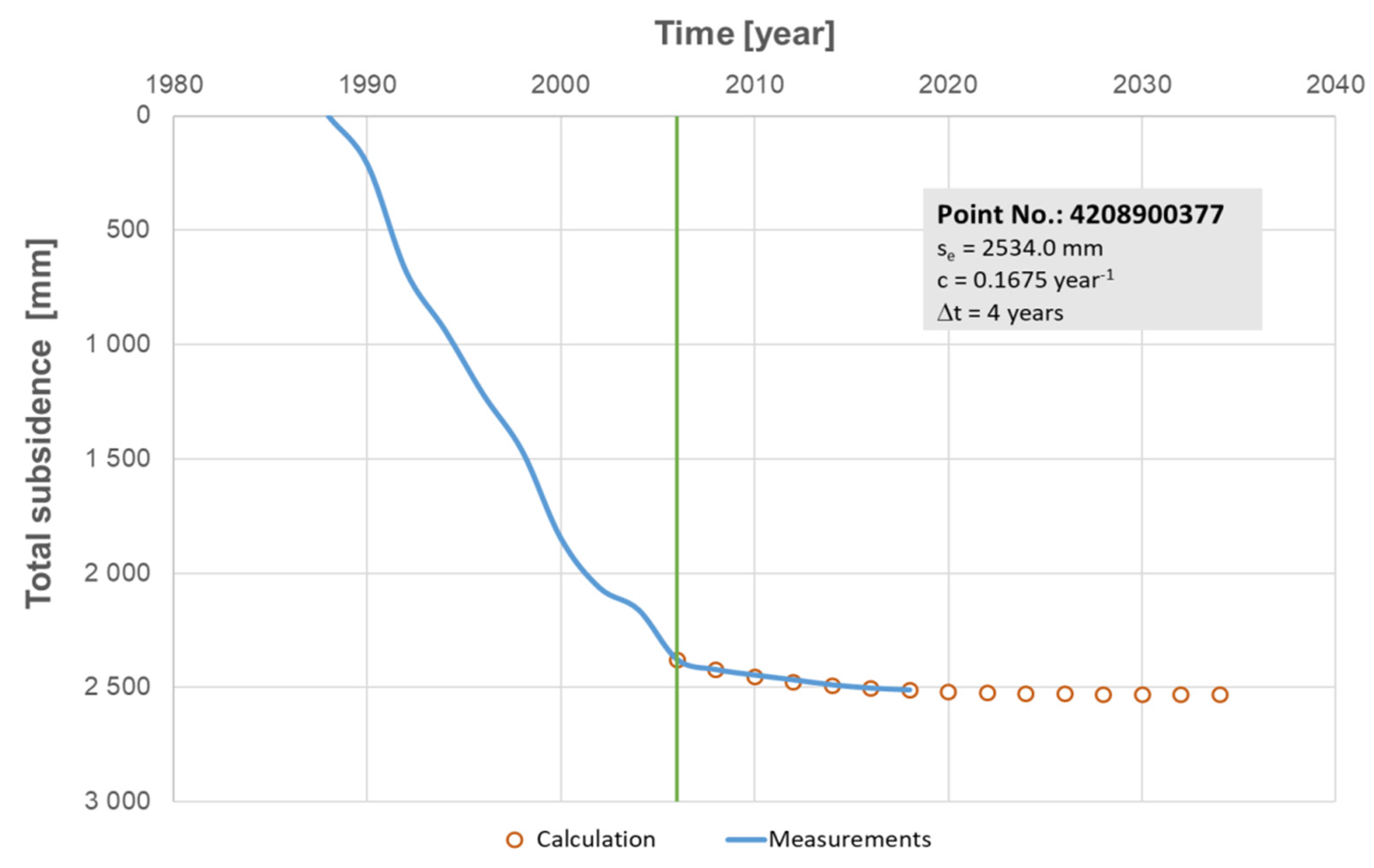
In order to present the calculation methodology using an example, the authors have included below a detailed description of the solution for the example of the measuring point number 4208900377. For the measurement data in Table 3, calculations were made for the three-point (Equations (3) and (4)) and four-point solution (Equations (7) and (8)). As a result of the calculations, the estimated values of the final subsidence of the residual point and additionally the time factor for individual calculation variants related to the time of measurements (with indicators standard deviations) were obtained:

• (four-point): measurements carried out in the years: 2008, 2010, 2016, and 2018; s_e = 2543.5 mm ± 20.5 mm, c = 0.1100 year⁻¹ ± 0.0279 year⁻¹, Δt = 2 years;
• (three-point): measurements carried out in the years: 2010, 2014, and 2018; s_e = 2534.0 mm ± 12.2 mm, c = 0.1675 year⁻¹ ± 0.0428 year⁻¹, Δt = 4 years;
• (three-point): measurements carried out in the years: 2006, 2012, and 2018; s_e = 2554.0 mm ± 11.2 mm, c = 0.1174 year⁻¹ ± 0.0141 year⁻¹, Δt = 6 years.

Performed calculations using the Gauss–Markov equalisation algorithm [52] according to the principle $\underset{\_}{v^{T}v}\to min!,$ where $v$ represents the difference between the modelled values of subsidence and the measured values.

Using all observations of subsidence from 2006 to 2018, they lead to the following results: s_e = 2546.2 mm ± 12.3 mm, c = 0.1300 year⁻¹ ± 0.0157 year⁻¹.

The results of the matching calculations are presented in

Table 4. Results of the subsidence obtained using the Gauss–Markov equalisation algorithm.

Year	Measured Subsidence [mm]	Model Subsidence [mm]	Difference (v) [mm]
2006	2378.00	2379.55	1.55
2008	2422.00	2417.71	−4.29
2010	2446.00	2447.13	1.13
2012	2467.00	2469.81	2.81
2014	2489.00	2487.30	−1.70
2016	2503.00	2500.79	−2.21
2018	2511.00	2511.19	0.19

.

The presented differences between the model subsidence calculated after identifying the parameters $s_e$, $c$, and the measured subsidence show that the error in determining a single subsidence is $s_0$ = 3.1 mm.

Noting that the mean values of the parameters $s_e$ and c calculated using the four and three point methods are $s_e$ = 2543.8 mm and $c$ = 0.1316 year⁻¹.

They are fully consistent with the results obtained on the basis of the Gauss–Markov algorithm.

For further analyses, option 2 was selected due to the calculated values and comparison of the graphs of forecasted subsidence. The predicted values of subsidence are presented in

Table 5. Forecast of subsidence for point 4208900377 after completion of measurements in 2018.

Year	Measured Subsidence [mm]	Calculated Subsidence [mm]
2008	2422.00	2411.00
2010	2446.00	2446.00
2012	2467.00	2471.10
2014	2489.00	2489.00
2016	2503.00	2501.80
2018	2511.00	2511.00
2020	-	2517.60
2022	-	2522.30
2024	-	2525.60
2026	-	2528.00
2028	-	2529.70
2030	-	2531.00

Sign “-” means that measurement was not carried out.

and in the diagram showing the course of subsidence (Figure 7).

The last stage of the calculations was to determine the expected time span for subsidence depending on the defined residual subsidence limit $\Delta s_{Gr}$. The results are presented in

Table 6. Estimated time of subsidence for subsidence limit values.

ΔsGr [mm] *	te(ΔsGr) [years]
100	-
50	2013
25	2017
10	2022
5	2027

Sign “-” means that measurement was not carried out * $\Delta s_{Gr}<s_e-s\left(t\right)$.

.

Figure 8, Figure 9 and Figure 10 below show graphical presentation of the results of forecasts for the remaining measurement points shown in Table 3.

Additionally,

Table 7. Subsidence time $t_e\left(\Delta s_{Gr}\right)$ depending on the residual subsidence limit $\Delta s_{Gr}$.

∆sGr [mm]	te(∆sGr)
	No. 4208900006	No. 4208900008	No. 4208900318	No. 4208900326	No. 4208900327	No. 4208900331	No. 4208900362	No. 4208900385	No. 4208900366
100	2012	2004	2004	2005	2005	2014	2012	2008	2015
50	2014	2016	2006	2011	2010	2016	2014	2010	2016
25	2016	2026	2010	2012	2012	2018	2016	2014	2017
10	2020	2038	2014	2014	2014	2020	2018	2016	2018
5	2022	2050	2018	2015	2016	2022	2020	2018	2020

presents the estimated subsidence time $t_e\left(\Delta s_{Gr}\right)$ for the individual measuring points, which depends on the defined residual subsidence limit $\Delta s_{Gr}$.

For residual subsidence limit $\Delta s_{Gr}$ = 50 mm, which was specified for agricultural land, subsidence was completed in 2014.

6. Discussion. Evaluation of the Time Function Based on the Results of In Situ Subsidence Measurements after the End of Mining Operations

The analyses presented above have shown that it is possible to forecast the residual subsidence after the end of the operation. On the other hand, the extensive observational material available to the authors allows for the evaluation of the applied time function. The analysis was carried out on the basis of any selected points from the analysed regions of mines located in the Ruhr Basin (Figure 11).

In mining practice, subsidence measurements are rarely performed at the end of a mining operation. For this reason, the starting point for the analyses is the first subsidence measurement made after its completion. Then, Equation (3) takes the form:

$$s\left(t\right)=s\left(t_1\right)+\left[s_e-s\left(t_1\right)\right]\left[1-exp\left(-c\left(t-t_1\right)\right)\right],t\ge T,$$

(17)

where $t_1$—time of the first measurement after the end of mining operations and $s\left(t_1\right)$—subsidence at the moment $t_1$.

The evaluation of the $s_e$ and $c$ parameters can be carried out using the approximate three- or four-point method and strictly using the Gauss–Markov equalisation algorithm. By transforming the equation, we arrive at:

$$\frac{s\left(t\right)-s\left(t_1\right)}{s_e-s\left(t_1\right)}=\frac{\Delta s\left(\Delta t\right)}{\Delta s_e}=1-exp\left(-c·\Delta t\right),$$

(18)

where $\mathsf{\Delta }t=t-t_1$.

Equation (18) leads to a time function of the form:

$$z\left(\Delta t\right)=1-exp\left(-c·\Delta t\right)$$

(19)

where $\mathsf{\Delta }t$—time after the end of mining operation (or after observation at time $t_1$).

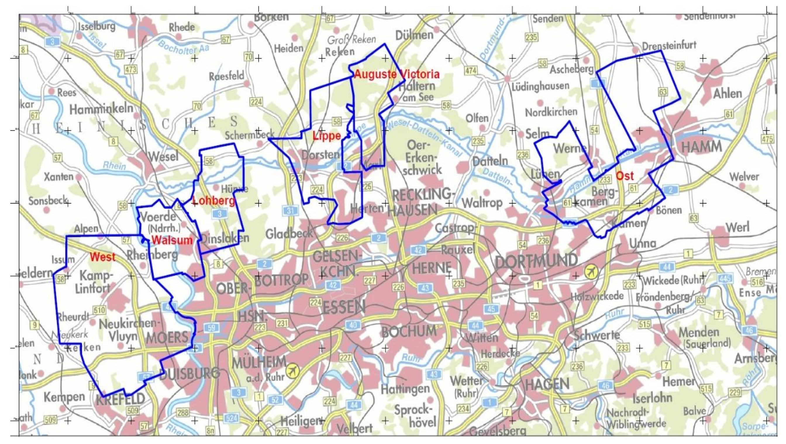
The evaluation of the above time function was based on the analysis of the subsidence course after the end of mining operations. The calculation results for six randomly selected individual points in the six analysed regions of the BW West Neu, BW Lippe, BW Ost, BW Walsum, BW Auguste-Victoria, and BW Loberg mines in the Ruhr Area are presented in

Table 8. Analysis of residual subsidence for selected points of various mines belonging to the RAG together with the determination of time coefficients.

Years	BW West Neu (Point 4505900101)			BW Lippe (Point 4308900148)			BW Ost (Point 4312900232)
	$\mathit{s}\mathbf{\left(}{\mathit{t}}_{\mathit{i}}\mathbf{\right)}$[mm]	$\frac{\mathsf{\Delta }\mathit{s}\mathbf{\left(}{\mathit{t}}_{\mathbf{1}}\mathbf{\right)}}{\mathsf{\Delta }{\mathit{s}}_{\mathit{e}}}$	$\mathit{c}\mathbf{·}\mathit{t}$	$\mathit{s}\mathbf{\left(}{\mathit{t}}_{\mathit{i}}\mathbf{\right)}$[mm]	$\frac{\mathsf{\Delta }\mathit{s}\mathbf{\left(}{\mathit{t}}_{\mathbf{1}}\mathbf{\right)}}{\mathsf{\Delta }{\mathit{s}}_{\mathit{e}}}$	$\mathit{c}\mathbf{·}\mathit{t}$	$\mathit{s}\mathbf{\left(}{\mathit{t}}_{\mathit{i}}\mathbf{\right)}$[mm]	$\frac{\mathsf{\Delta }\mathit{s}\mathbf{\left(}{\mathit{t}}_{\mathbf{1}}\mathbf{\right)}}{\mathsf{\Delta }{\mathit{s}}_{\mathit{e}}}$	$\mathit{c}\mathbf{·}\mathit{t}$
1994	2553	0.0000	0.0000	-	-	-	-	-
2000	2607	0.2795	0.3282	-	-	-	-	-
2002	-	-	-	-	-	-	-	-
2004	-	-	-	-	-	-	740	0.0000	0.0000
2006	2646	0.4814	0.6564	-	-	-	782	0.3043	0.3590
2008		-	-	-	-	-	813	0.5290	0.7180
2010		-	-	4820	0.0000	0.0000	831	0.6594	1.0770
2012	2674	0.6263	0.9846	4839	0.3333	0.4054	840	0.7246	1.4360
2014	-	-	-	4853	0.5789	0.8108	850	0.7971	1.7950
2016	-	-	-	4861	0.7193	1.2162	862	0.8841	2.1540
2018	-	-	-	-	-	-	865	0.9058	2.5130
Years	BW Walsum (Point 4405900174)			BW Auguste-Victoria (Point 4208900008)			BW Loberg (Point 4406900209)
	$\mathit{s}\mathbf{\left(}{\mathit{t}}_{\mathit{i}}\mathbf{\right)}$[mm]	$\frac{\mathsf{\Delta }\mathit{s}\mathbf{\left(}{\mathit{t}}_{\mathbf{1}}\mathbf{\right)}}{\mathsf{\Delta }{\mathit{s}}_{\mathit{e}}}$	$\mathit{c}\mathit{t}$	$\mathit{s}\mathbf{\left(}{\mathit{t}}_{\mathit{i}}\mathbf{\right)}$[mm]	$\frac{\mathsf{\Delta }\mathit{s}\mathbf{\left(}{\mathit{t}}_{\mathbf{1}}\mathbf{\right)}}{\mathsf{\Delta }{\mathit{s}}_{\mathit{e}}}$	$\mathit{c}\mathit{t}$	$\mathit{s}\mathbf{\left(}{\mathit{t}}_{\mathit{i}}\mathbf{\right)}$[mm]	$\frac{\mathsf{\Delta }\mathit{s}\mathbf{\left(}{\mathit{t}}_{\mathbf{1}}\mathbf{\right)}}{\mathsf{\Delta }{\mathit{s}}_{\mathit{e}}}$	$\mathit{c}\mathit{t}$
1994	-	-	-	-	-	-	-	-	-
2000	2171	0.0000	0.0000	-	-	-	-	-	-
2002	-	-	-	795	0.0000	0.0000	-	-	-
2004	-	-	-	809	0.1228	0.1352	-	-	-
2006	2281	0.3714	0.4470	825	0.2632	0.2704	1274	0.0000	0.0000
2008	-	-	-	833	0.3333	0.4056	1314	0.1899	0.2164
2010	-	-	-	839	0.3860	0.5408	1348	0.3514	0.4328
2012	2346	0.5908	0.8940	849	0.4737	0.6760	1371	0.4606	0.6492
2014	-	-	-	860	0.5702	0.8112	1396	0.5793	0.8656
2016	-	-	-	866	0.6228	0.9464	1410	0.6458	1.0820
2018	2391	0.7427	1.3410	869	0.6491	1.0816	1427	0.7265	1.2984

Sign “-” means that measurement was not carried out.

and collectively in Figure 12.

For each analysed area of mines, the values of $s_e$ and $c$ parameters were determined, adopting the methodology presented in the article:

• BW West Neu: s_e = 2746.2 mm ± 20.6 mm, c = 0.0547 year⁻¹ ± 0.0086 year⁻¹, Δt = 6 years;
• BW Lippe: s_e = 4877.0 mm ± 6.1 mm, c = 0.2027 year⁻¹ ± 0.1318 year⁻¹, Δt = 2 years;
• BW Ost: s_e = 878.0 mm ± 5.6 mm, c = 0.1795 year⁻¹ ± 0.0184 year⁻¹, Δt = 2 years;
• BW Walsum: s_e = 2467.2 mm ± 11.6 mm, c = 0.0745 year⁻¹ ± 0.0057 year⁻¹, Δt = 6 years;
• BW Auguste-Victoria: s_e = 909.0 mm ± 17.2 mm, c = 0.0676 year⁻¹ ± 0.0157 year⁻¹, Δt = 2 years;
• BW Loberg: s_e = 1484.6 mm ± 27.4 mm, c = 0.1082 year⁻¹ ± 0.0212 year⁻¹, Δt = 2 years.

Table 8 summarises the calculated values of $\frac{\Delta s\left(t_1\right)}{\Delta s_e}$ and $c·t$ for selected points of six mines belonging to the RAG company, where $\Delta s_e=s_e-s\left(t_1\right)$.

Based on the data presented in Table 8, a graph of the time function was prepared (Figure 12).

7. Summary

Forecasting the residual movements of the land surface caused by mining operations is essential for determining the period of measurements and for assessing the potential mining damage and the possibility of reusing the land. The experiences of the international scientists cited at the beginning of the article do not give a clear indication of the time span that should be taken to determine long-term residual subsidence. The presented calculation example for the actual mine owned by RAG (Auguste-Victoria), based on the author’s solution, shows that in some cases this time may continue for several years. Observations of the measurements and results of calculations indicate that after the closure of the Auguste-Victoria mine, the measured differences in subsidence in the 2014–2016 and 2016–2018 measurement periods are clearly decreasing compared to the previous period. The predicted average increase in subsidence over the period 2018–2020 is about 5 mm, and the expected value of maximum subsidence will be at about 20 mm, i.e., 10 mm per year. These values are not significant for building structures, while for agriculture, assuming a residual subsidence limit of $\Delta s_{Gr}$ = 50 mm, it was estimated that surface movements ended in 2014.