
A FORTRAN Program to Model Magnetic Gradient Tensor at High Susceptibility Using Contraction Integral Equation Method


Abstract
1. Introduction
2. Contraction Integral Equation Method
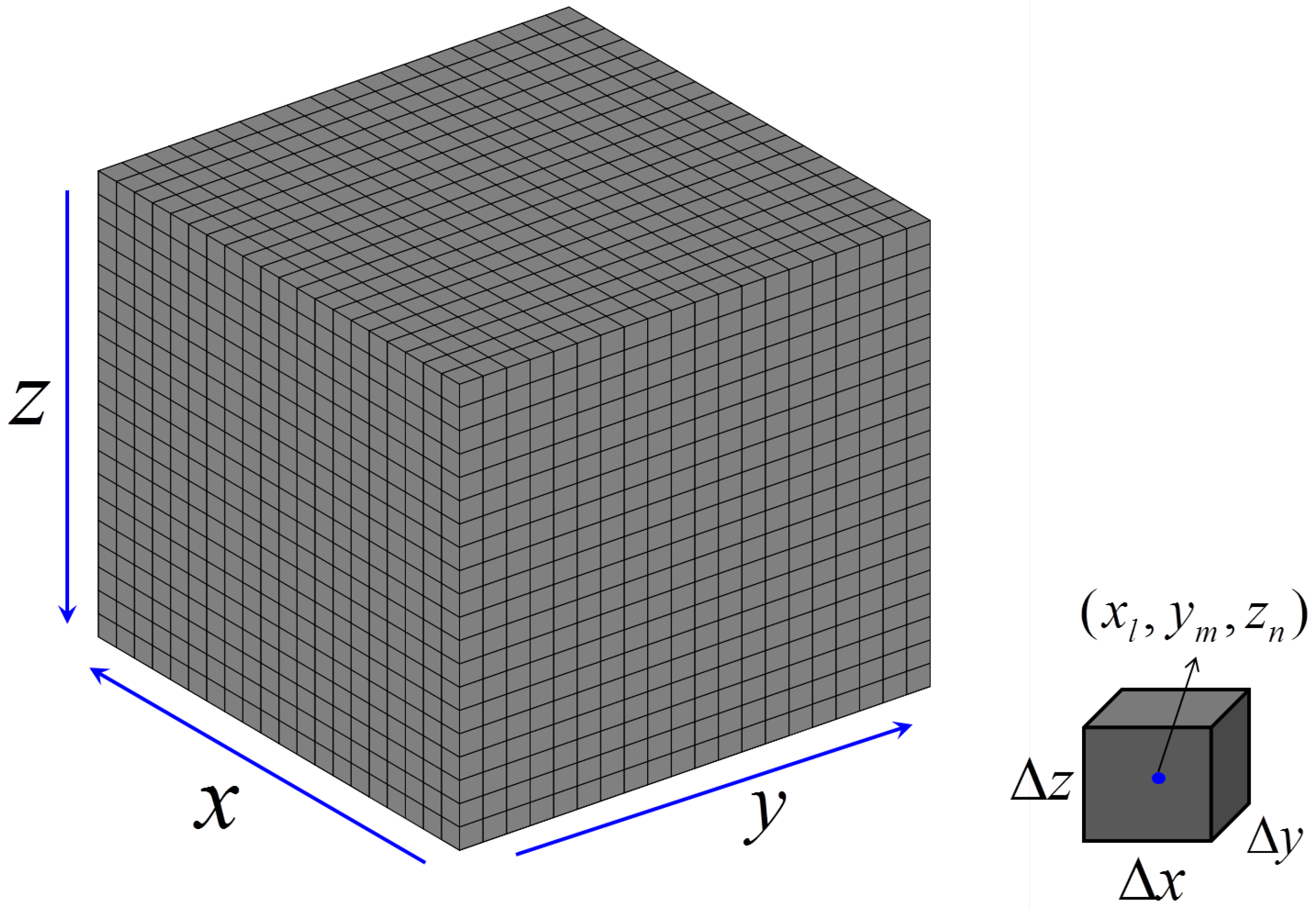
2.1. The Integral Equation
2.2. Iterative Scheme
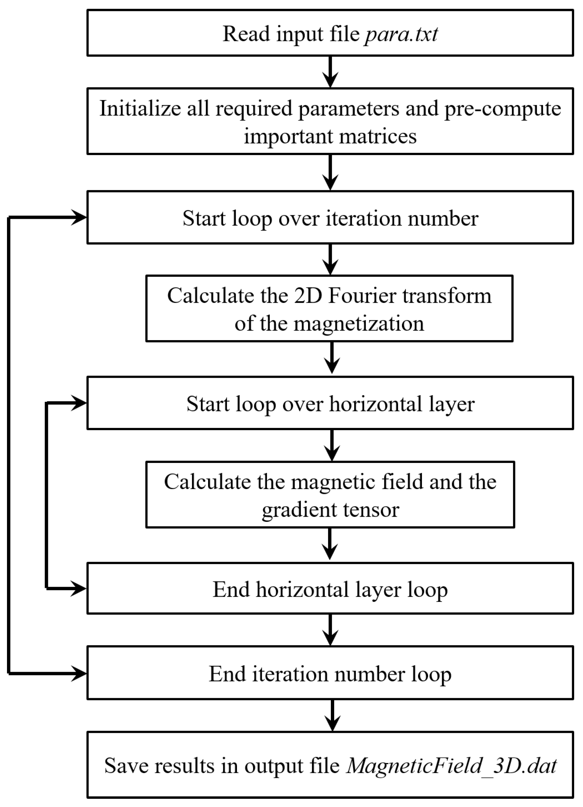
2.3. Workflow for Modeling Gradient Fields
3. Description of The Code
3.1. Subroutines
3.2. Inputs and Outputs
4. Numerical Tests
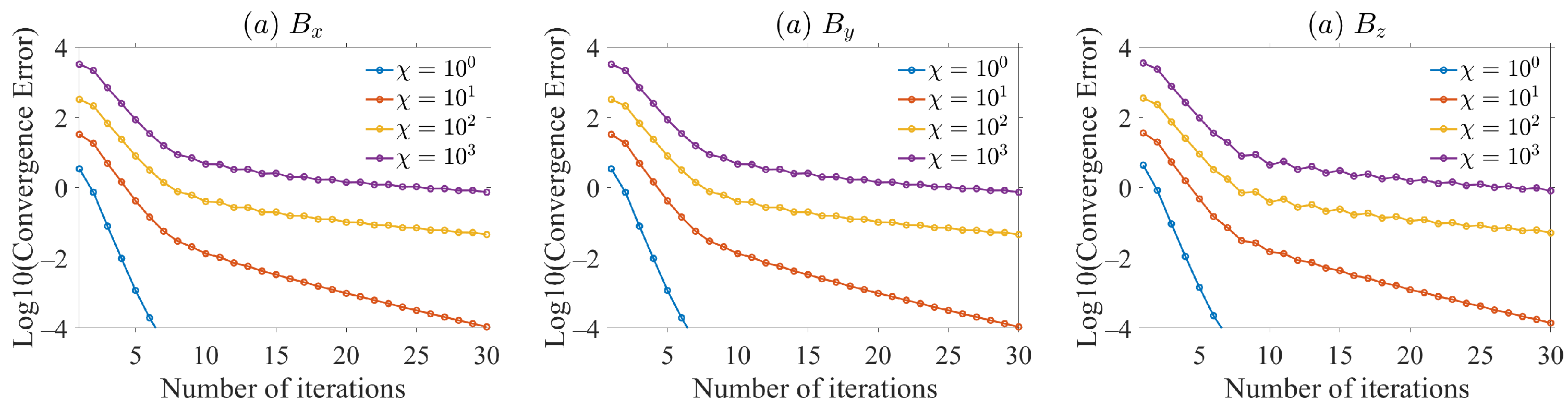
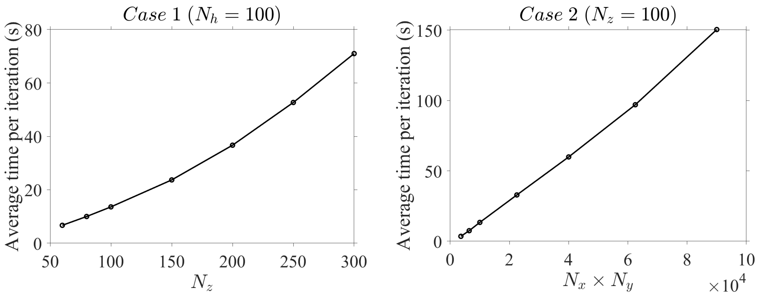
4.1. Performance
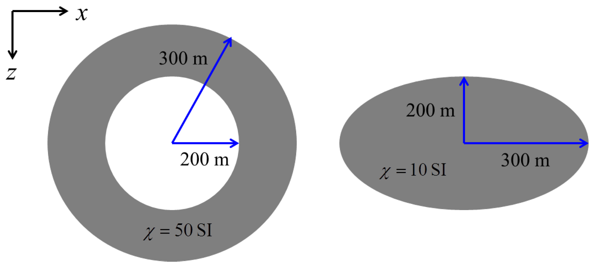
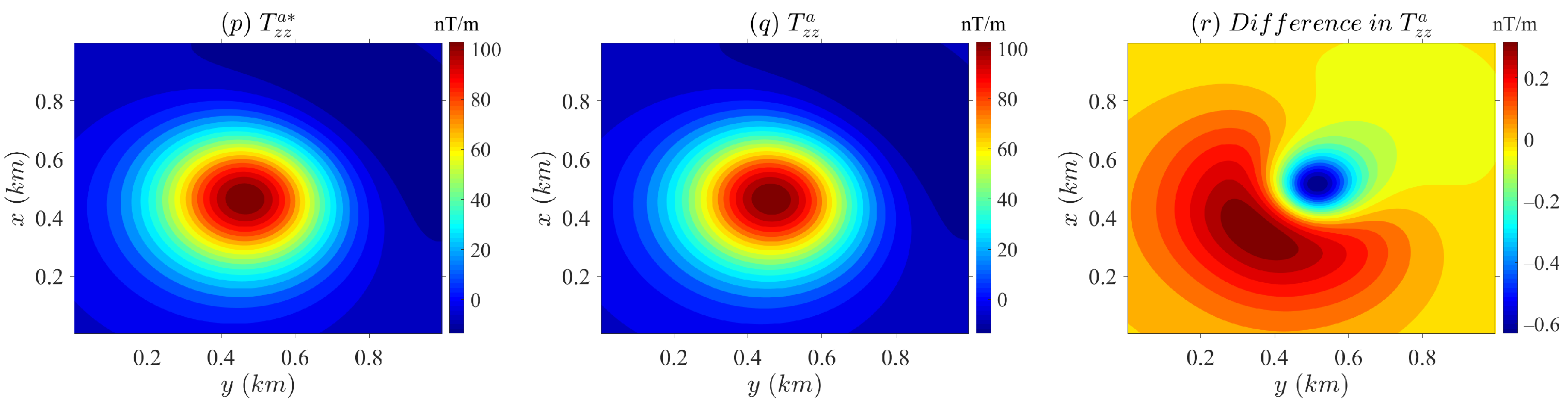
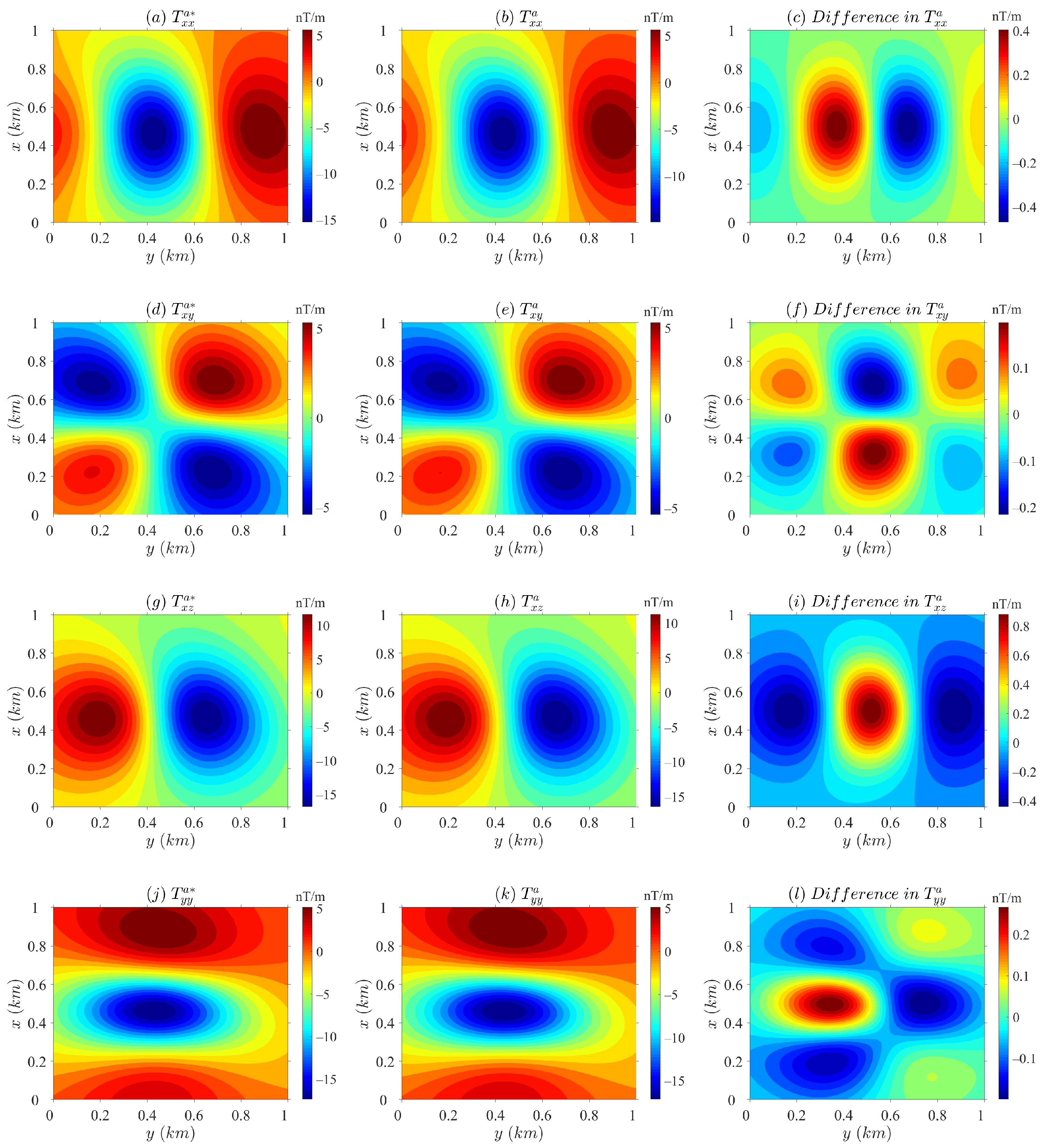
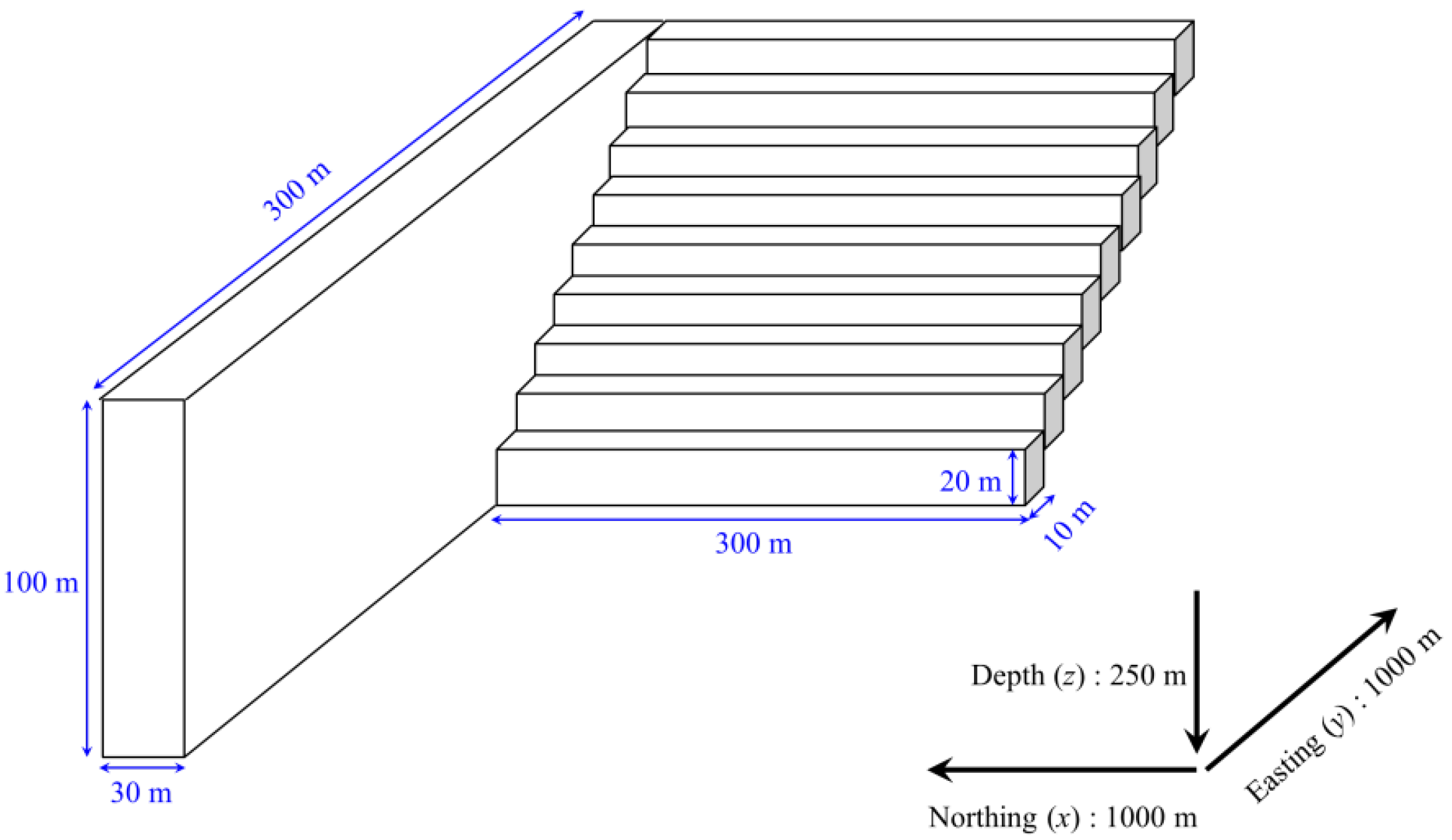
4.2. Example
5. Conclusions
Author Contributions
Funding
Institutional Review Board Statement
Informed Consent Statement
Data Availability Statement
Acknowledgments
Conflicts of Interest
Appendix A. Analytical Solutions
References
- Wang, Y.F.; Rong, L.L.; Qiu, L.Q.; Lukyanenko, D.V.; Yagola, A.G. Magnetic susceptibility inversion method with full tensor gradient data using low-temperature SQUIDs. Pet. Sci. 2019, 16, 794–807. [Google Scholar] [CrossRef]
- Schmidt, P.W.; Clark, D.A.; Leslie, K.E.; Bick, M.; Tilbrook, D.L. GET-MAG-a SQUID magnetic tensor gradiometer for mineral and oil exploration. Explor. Geophys. 2004, 35, 297–305. [Google Scholar] [CrossRef]
- Stocco, S.; Godio, A.; Sambuelli, L. Modelling and compact inversion of magnetic data: A Matlab code. Comput. Geosci. 2009, 35, 2111–2118. [Google Scholar] [CrossRef]
- Zhdanov, M.S.; Cai, H.Z.; Wilson, G.A. Migration transformation of two-dimensional magnetic vector and tensor fields. Geophys. J. Int. 2012, 189, 1361–1368. [Google Scholar] [CrossRef][Green Version]
- Schiffler, M.; Queitsch, M.; Stolz, R.; Chwala, A.; Krech, W.; Meyer, H.G.; Kukowski, N. Calibration of SQUID vector magnetometers in full tensor gradiometry systems. Geophys. J. Int. 2014, 198, 954–964. [Google Scholar] [CrossRef]
- Brown, P.J.; Bracken, R.E.; Smith, D.V. A case study of magnetic gradient tensor invariants applied to the UXO problem. In Proceedings of the SEG International Exposition and 74th Annual Meeting, Denver, CO, USA, 10–15 October 2004; pp. 794–797. [Google Scholar]
- Stolz, R.; Zakosarenko, V.; Schulz, M.; Chwala, A.; Frtitzsch, L.; Meyer, H.G.; Kostlin, E.O. Magnetic full-tensor SQUID gradiometer system for geophysical applications. Lead. Edge 2006, 25, 178–180. [Google Scholar] [CrossRef]
- Schmidt, P.W.; Clark, D.A. Advantages of measuring the magnetic gradient tensor. Preview 2000, 85, 26–30. [Google Scholar]
- Heath, P.J.; Heinson, G.; Greenhalgh, S.A. Some comments on potential field tensor data. Explor. Geophys. 2003, 34, 57–62. [Google Scholar] [CrossRef]
- Schmidt, P.W.; Clark, D.A. The magnetic gradient tensor: Its properties and uses in source characterization. Lead. Edge 2006, 25, 75–78. [Google Scholar] [CrossRef]
- Kotsiaros, S.; Olsen, N. The geomagnetic field gradient tensor properties and parametrization in terms of spherical harmonics. Int. J. Geomath. 2012, 3, 297–314. [Google Scholar] [CrossRef]
- Bhattacharyya, B.K. Magnetic anomalies due to prism-shaped bodies with arbitrary polarization. Geophysics 1964, 29, 517–531. [Google Scholar] [CrossRef]
- Clark, D.A.; Saul, S.J.; Emerson, D.W. Magnetic and gravity anomalies of a triaxial ellipsoid. Explor. Geophys. 1986, 17, 189–200. [Google Scholar] [CrossRef]
- Blakely, R.J. Potential Theory In Gravity And Magnetic Applications; Cambridge University Press: Cambridge, UK, 1996; pp. 154–196. [Google Scholar]
- Halliday, D.; Resnick, R.; Walker, J. Fundamentals of Physics; John Wiley and Sons: New York, NY, USA, 1997. [Google Scholar]
- Sharma, P.V. Demagnetization effect of a rectangular prism. Geophysics 1968, 33, 132–134. [Google Scholar] [CrossRef]
- Eskola, L.; Tervo, T. Solving the magnetostatic field problem (a case of high susceptibility) by means of the method of subsections. Geo-Exploration 1980, 18, 79–95. [Google Scholar] [CrossRef]
- Lee, T.J. Rapid computation of magnetic anomalies with demagnetization included, for arbitarily shaped magnetic bodies. Geophys. J. R. Astron. Soc. 1980, 60, 67–75. [Google Scholar] [CrossRef]
- Furness, P. A versatile integral equation technique for magnetic modeling. J. Appl. Geophys. 1999, 41, 345–357. [Google Scholar] [CrossRef]
- Butler, D.K.; Pasion, L.; Billings, S.; Oldenburg, D.; Yule, D. Enhanced discrimination capability for UXO geophysical surveys. In Proceedings of the SPIE Detection and Remediation Technologies and Mines and Minelike Targets VIII, Orlando, FL, USA, 21–25 April 2003; pp. 958–969. [Google Scholar]
- Sanchez, V.; Li, Y.; Nabighian, M.N.; Wright, D.L. Numerical modeling of higher order magnetic moments in UXO discrimination. IEEE Trans. Geosci. Remote Sens. 2008, 46, 2568–2583. [Google Scholar] [CrossRef]
- Baykiev, E.; Ebbing, J.; Bronner, M.; Fabian, K. Forward modeling magnetic fields of induced and remanent magnetization in the lithosphere using tesseroids. Comput. Geosci. 2016, 96, 124–135. [Google Scholar] [CrossRef]
- Chen, L.W.; Liu, L.B. Fast and accurate forward modelling of gravity field using prismatic grids. Geophys. J. Int. 2019, 216, 1062–1071. [Google Scholar] [CrossRef]
- Hogue, J.D.; Renaut, R.A.; Vatankhah, S. A tutorial and open source software for the efficient evaluation of gravity and magnetic kernels. Comput. Geosci. 2020, 144, 104575. [Google Scholar] [CrossRef]
- Bhattacharyya, B.K.; Navolio, M.E. A fast Fourier transform method for rapid computation of gravity and magnetic anomalies due to arbitrary bodies. Geophys. Prospect. 1976, 24, 633–649. [Google Scholar] [CrossRef]
- Tontini, F.C. Rapid interactive modeling of 3D magnetic anomalies. Comput. Geosci. 2012, 48, 308–315. [Google Scholar] [CrossRef]
- Wu, L.Y.; Tian, G. High-precision Fourier forward modeling of potential fields. Geophysics 2014, 79, G59–G68. [Google Scholar] [CrossRef]
- Purss, M.B.J.; Cull, J.P. A new iterative method for computing the magnetic field at high magnetic susceptibilities. Geophysics 2005, 70, L53–L62. [Google Scholar] [CrossRef]
- Krahenbubl, R.A.; Li, Y. Investigation of magnetic inversion methods in highly magnetic environments under strong self-demagnetization effect. Geophysics 2017, 82, J83–J97. [Google Scholar] [CrossRef]
- Ouyang, F.; Chen, L.W. Iterative magnetic forward modeling for high susceptibility based on integral equation and Gauss-fast Fourier transform. Geophysics 2020, 85, J1–J13. [Google Scholar] [CrossRef]
- Lelievre, P.G.; Oldenburg, D.W. Magnetic forward modeling and inversion for high susceptibility. Geophys. J. Int. 2006, 166, 76–90. [Google Scholar] [CrossRef]
- Ren, Z.Y.; Chen, C.J.; Tang, J.T.; Chen, H.; Hu, S.G.; Zhou, C.; Xiao, X. Closed-form formula of magnetic gradient tensor for a homogeneous polyhedral magnetic target: A tetrahedral grid example. Geophysics 2017, 82, WB21–WB28. [Google Scholar] [CrossRef]
- Ren, Z.Y.; Chen, H.; Chen, C.J.; Zhong, Y.Y.; Tang, J.T. New analytical expression of the magnetic gradient tensor for homogeneous polyhedron. Geophysics 2019, 84, A31–A35. [Google Scholar] [CrossRef]
- Guo, W.; Dentith, M.; Bird, R.T.; Clark, D.A. Systematic error analysis of demagnetization and implications for magnetic interpretation. Geophysics 2001, 66, 562–570. [Google Scholar] [CrossRef]
- Butler, D.K.; Wolfe, P.J.; Hansen, R.O. Analytical modeling of magnetic and gravity signatures of unexploded ordnance. J. Environ. Eng. Geophys. 2001, 6, 33–46. [Google Scholar] [CrossRef]
- Tomazella, D.; Oliveira, V.C., Jr. Ellipsoids (v1.0): 3D magnetic modelling of ellipsoidal bodies. Geosci. Model Dev. Discuss. 2017, 10, 3591–3608. [Google Scholar]


| Main Program | Main | Perform the Iterative Procedure and Calculate the Magnetic Gradient Tensor |
|---|---|---|
| Major subroutines | ReadIn | Initialize all required parameters and read model parameters from the input file (para.txt). |
| Storage | Pre-compute and save important matrices. | |
| Wavenumber | Generate wavenumbers for the 2D Gauss-FFT. | |
| Background | Set background fields. | |
| Model | Establish a model. | |
| GaussFFT_2D_Fast | Achieve forward and inverse 2D Gauss-FFT. | |
| Major subroutines | Module | Include initial variable declarations. |
| Coordinates | Generate rectangular prims. | |
| Output | Output the calculation results, including six gradient field components and three magnetic field components. | |
| DeOrAllocate | Allocate and deallocate parameters. |
| Nx, Ny, Nz | Number of prismatic elements in the x, y and z directions. |
|---|---|
| z0 | The minimum z coordinate of geometric center of prisms (m). |
| x1, y1, z1 | The maximum x, y and z coordinates of geometric center of prisms (m). |
| NI | Maximum number of iterations |
| NG | Number of Gaussian nodes used in 2D Gauss-FFT (NG = 1, 2, 3 or 4) |
| Ang1 | Inclination angle (degree) |
| Ang2 | Declination angle (degree) |
| Bgr | Strength of the inducing field (nT) |
| Gradient Fields | Min (nT) | Max (nT) | Rms | Rrms * (%) | ||||
|---|---|---|---|---|---|---|---|---|
| Shell | Ellipsoid | Shell | Ellipsoid | Shell | Ellipsoid | Shell | Ellipsoid | |
| −54.188 | −14.931 | 19.733 | 6.691 | 0.082 | 0.158 | 0.455 | 2.812 | |
| −17.159 | −5.358 | 18.884 | 5.818 | 0.046 | 0.079 | 0.467 | 2.533 | |
| −54.908 | −16.482 | 44.953 | 12.703 | 0.094 | 0.276 | 0.431 | 4.031 | |
| −54.188 | −17.190 | 19.733 | 6.210 | 0.082 | 0.092 | 0.455 | 1.534 | |
| −54.908 | −16.983 | 44.953 | 13.923 | 0.094 | 0.177 | 0.431 | 2.459 | |
| −13.582 | −5.235 | 108.377 | 32.115 | 0.142 | 0.565 | 0.457 | 5.538 | |
Publisher’s Note: MDPI stays neutral with regard to jurisdictional claims in published maps and institutional affiliations. |
© 2021 by the authors. Licensee MDPI, Basel, Switzerland. This article is an open access article distributed under the terms and conditions of the Creative Commons Attribution (CC BY) license (https://creativecommons.org/licenses/by/4.0/).
Share and Cite
Chen, L.; Ouyang, F. A FORTRAN Program to Model Magnetic Gradient Tensor at High Susceptibility Using Contraction Integral Equation Method. Minerals 2021, 11, 1129. https://doi.org/10.3390/min11101129
Chen L, Ouyang F. A FORTRAN Program to Model Magnetic Gradient Tensor at High Susceptibility Using Contraction Integral Equation Method. Minerals. 2021; 11(10):1129. https://doi.org/10.3390/min11101129
Chicago/Turabian StyleChen, Longwei, and Fang Ouyang. 2021. "A FORTRAN Program to Model Magnetic Gradient Tensor at High Susceptibility Using Contraction Integral Equation Method" Minerals 11, no. 10: 1129. https://doi.org/10.3390/min11101129
APA StyleChen, L., & Ouyang, F. (2021). A FORTRAN Program to Model Magnetic Gradient Tensor at High Susceptibility Using Contraction Integral Equation Method. Minerals, 11(10), 1129. https://doi.org/10.3390/min11101129