
Emplacement and Segment Geometry of Large, High-Viscosity Magmatic Sheets

 , ,
, ,
Abstract
1. Introduction
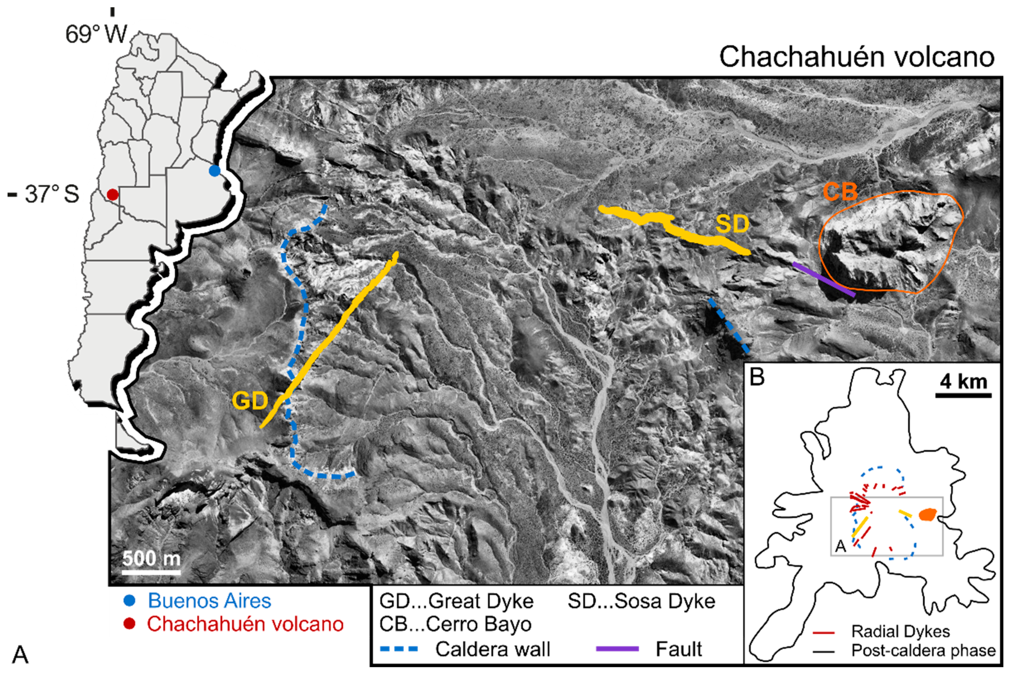
2. Geological Setting
3. Methods
3.1. Field Work and Photogrammetry
3.2. Rock Samples and AMS Analysis
3.3. Geochemistry and Petrographic Analysis
4. Results
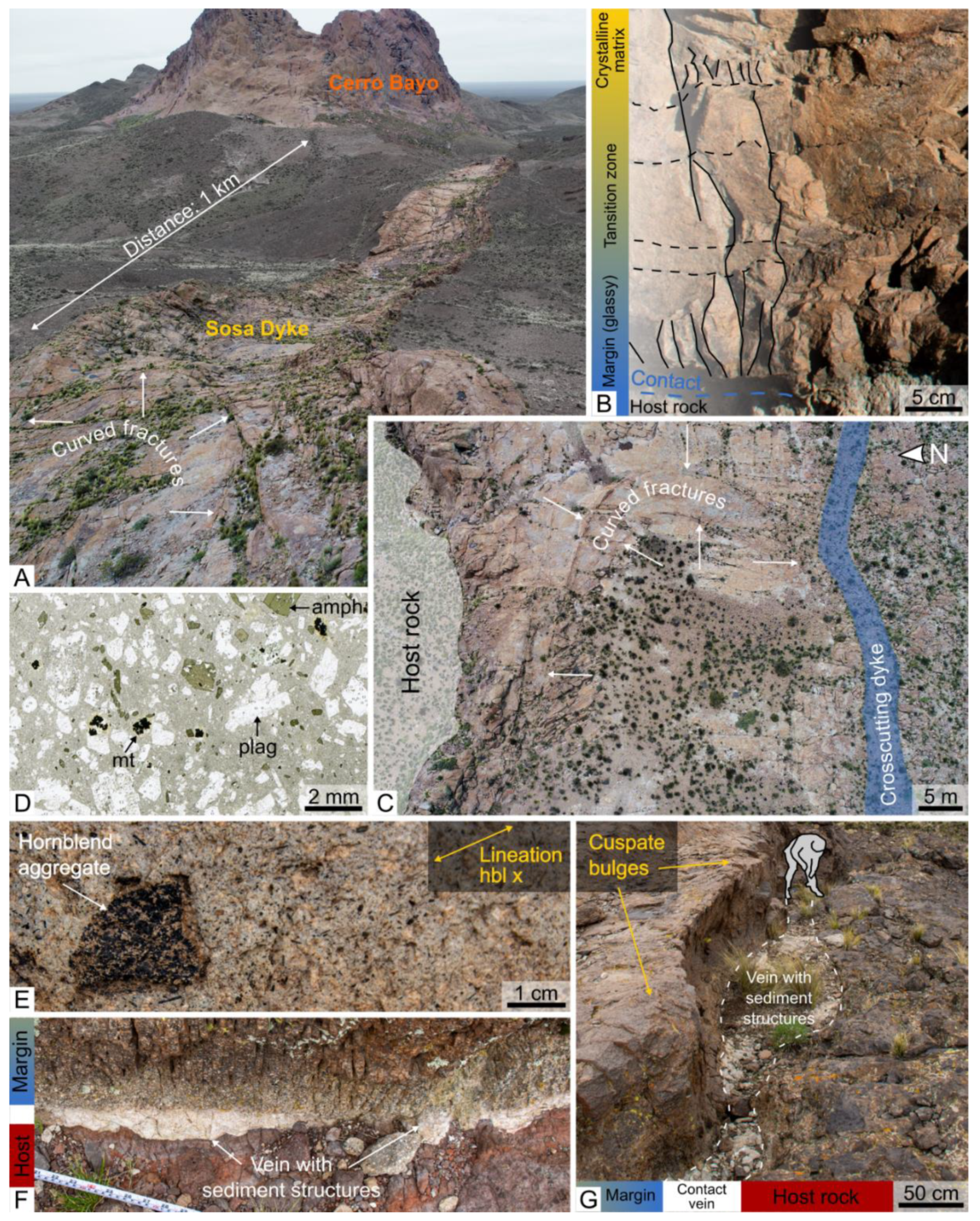
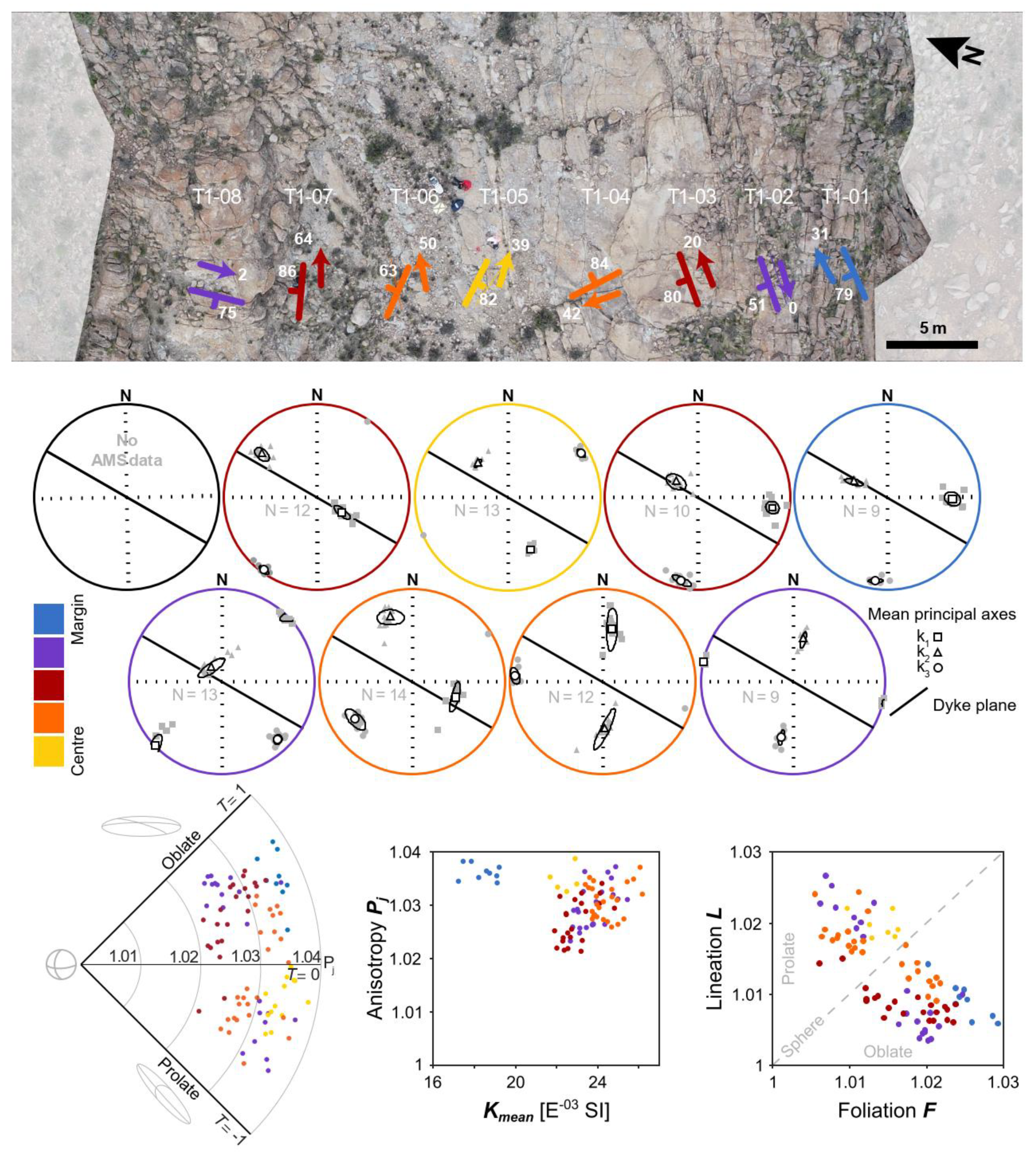
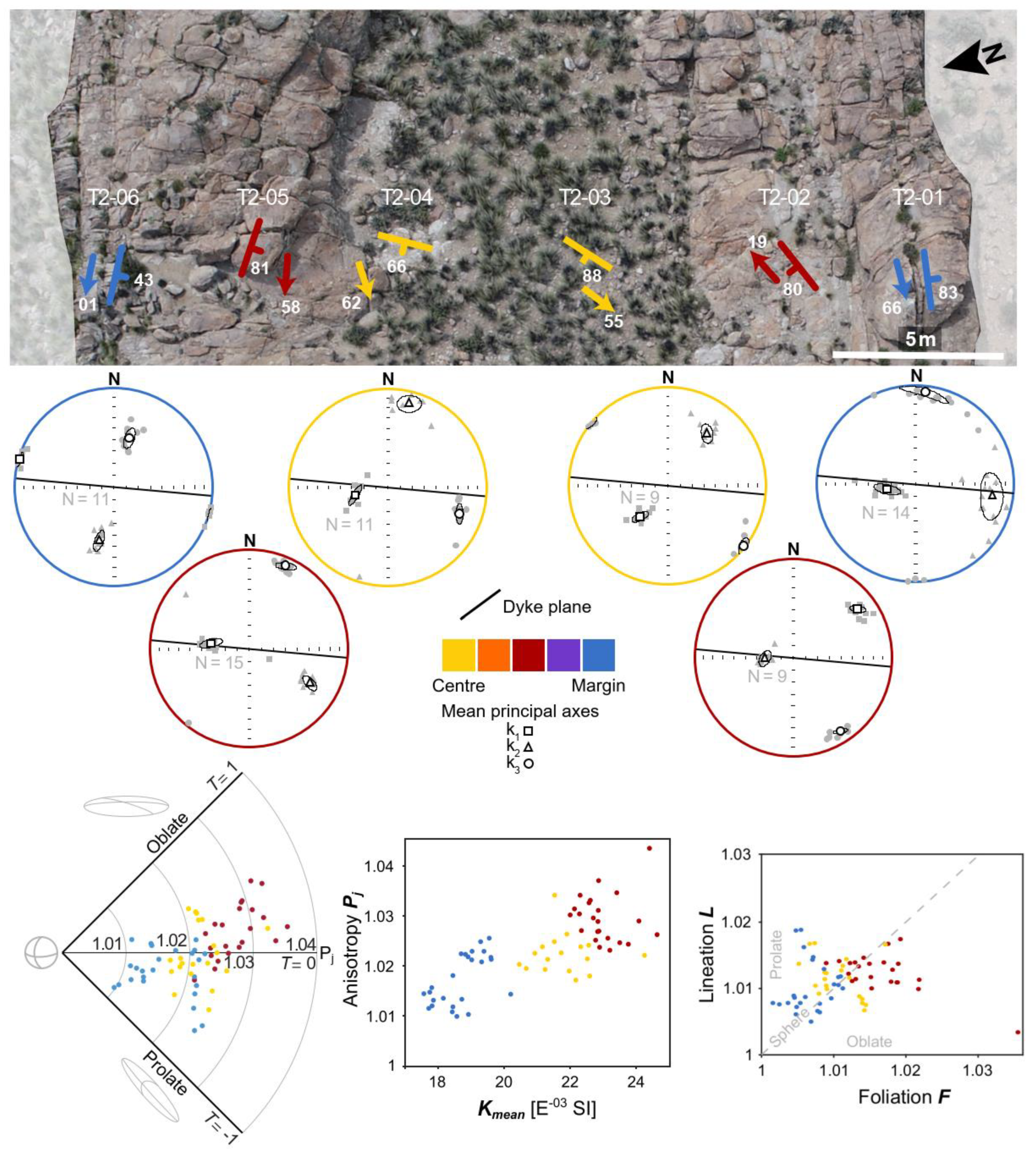
4.1. Sosa Dyke
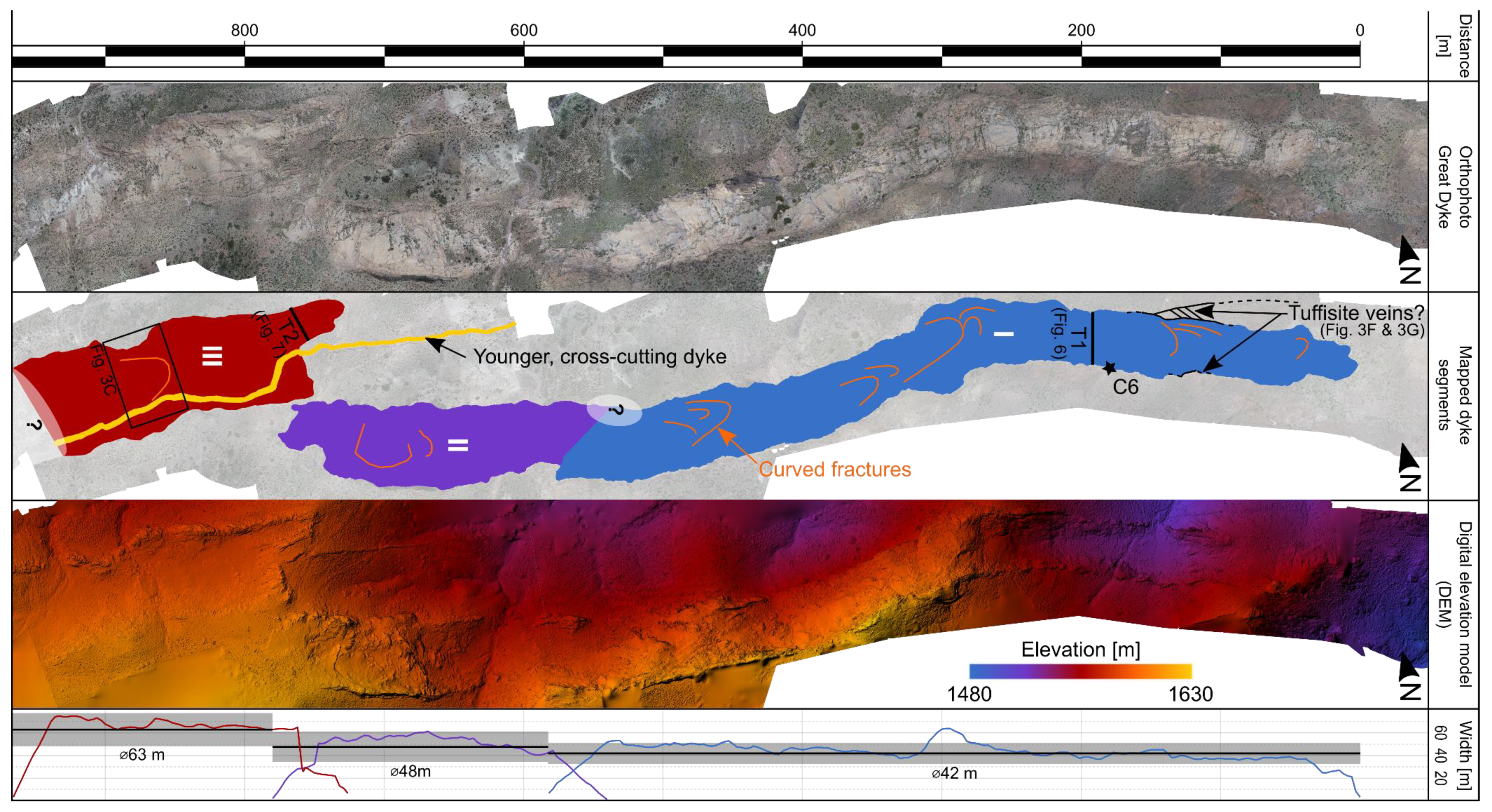
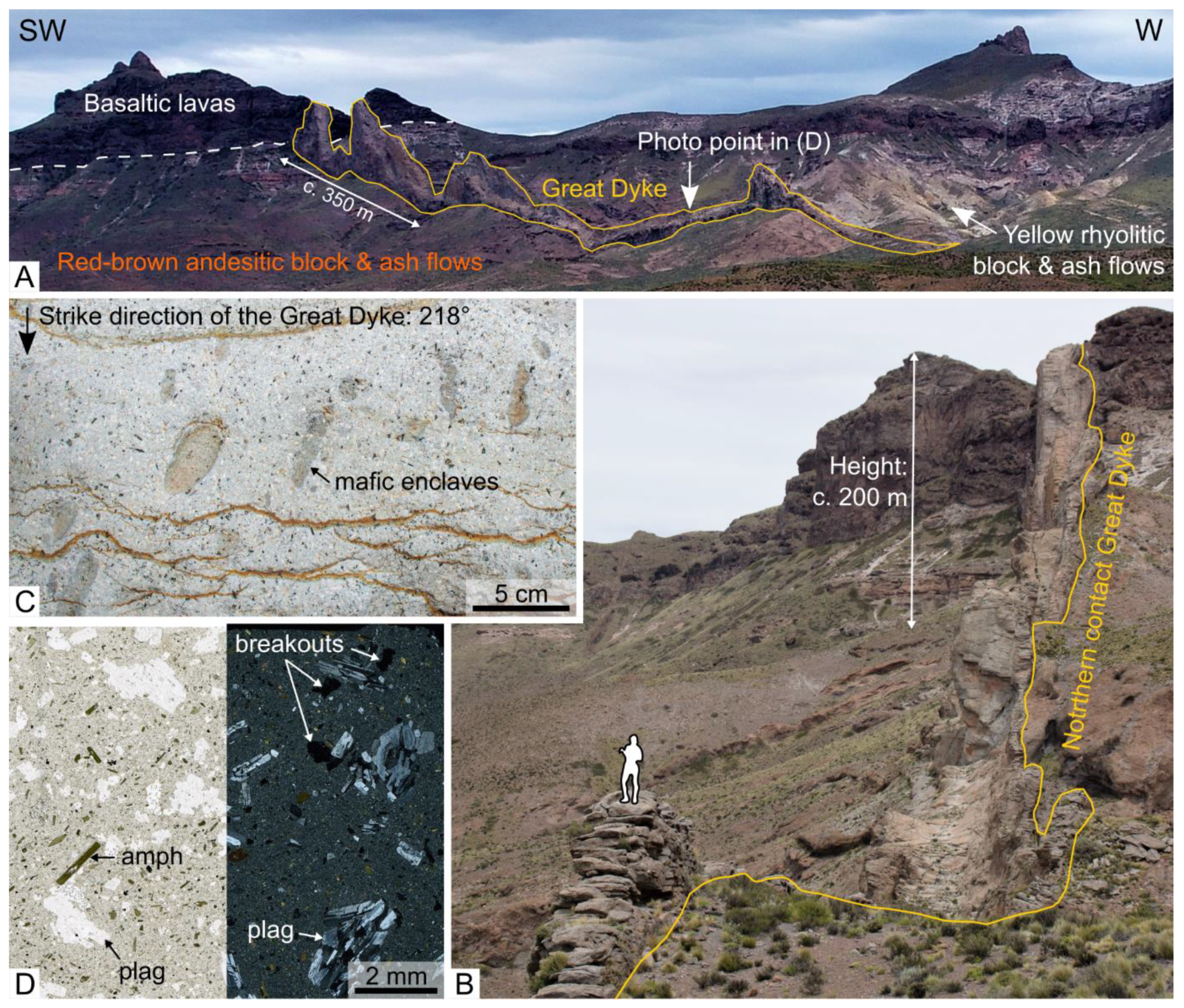
4.2. Great Dyke
4.3. Anisotropy of Magnetic Susceptibility (AMS)
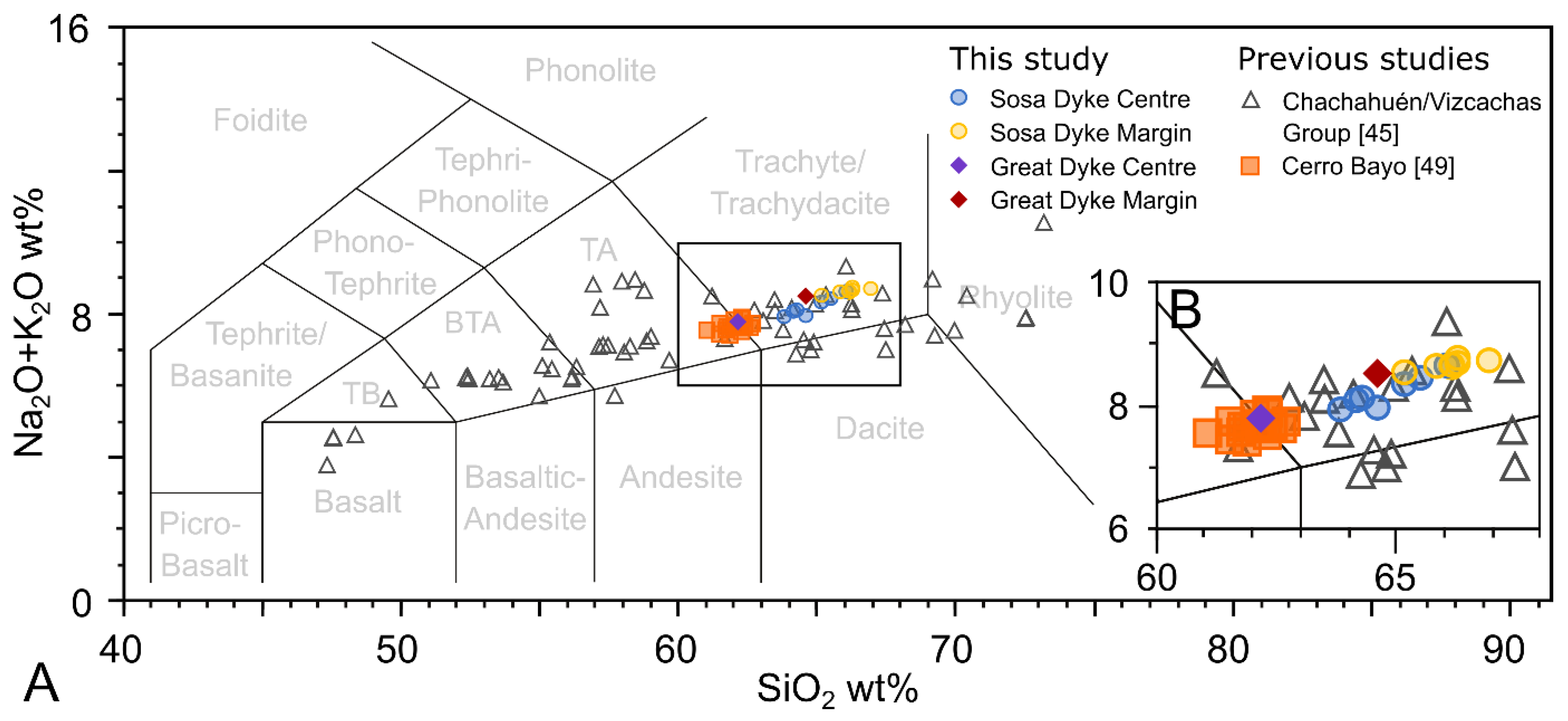
4.4. Geochemistry
4.5. Viscosity
5. Interpretation/Discussion
5.1. Segment Offset—Initial Dyke Geometry or Tectonic Feature?
5.2. Interpretation of Magma Flow Direction in the Sosa Dyke
5.3. High-Viscosity Sheet Intrusions and the Effect of Different Host Rocks on the Intrusion Geometry
5.4. Segment Geometry and Dyke Emplacement
6. Conclusions
- The segment geometries observed in this study are related to the emplacement of the dykes, rather than the result of post-emplacement tectonic deformation;
- AMS and curved fractures record a dominant lateral magma flow direction in the Sosa Dyke towards the East, thus contradicting expected vertical magma flow derived from dyke segment geometry. It remains unsolved if the flow indicators thus record a late-stage of a dominantly vertical dyke emplacement or an overall lateral dyke emplacement;
- The comparison between low- to high-viscosity magma sheet segment geometries reveal a significant similarity. Thus, we question the common practice of using sheet segment geometries as proxies for different intrusion emplacement mechanisms of low- and high-viscosity sheet intrusions;
- The similarities between low- and high-viscosity sheets emplaced within host rocks of different strengths suggest that magma sheet emplacement is governed not only by the magma viscosity or the host rock strength, but by the balance between the viscous stresses within the flowing magma and the deforming host rock. The final intrusion shape is not sufficient to reveal the entire emplacement history of magmatic sheet intrusions.
Supplementary Materials
Author Contributions
Funding
Data Availability Statement
Acknowledgments
Conflicts of Interest
Appendix A. Whole Rock Geochemistry and Fourier Transform Infrared Spectroscopy (FTIR) Analysis
Appendix A.1. Whole Rock Geochemistry

| Sosa Dyke (GD) | |||||||||
|---|---|---|---|---|---|---|---|---|---|
| SAMPLE | T1-01 | T1-02 | T1-03 | T1-04 | T1-05 | T1-06 | T1-07 | T1-08 | T1-09 |
| SiO2 (wt%) | 64.7 | 65.1 | 64.1 | 63.2 | 63.6 | 62.9 | 63.3 | 64.1 | 65.0 |
| Al2O3 | 17.60 | 17.75 | 17.60 | 17.30 | 17.40 | 17.25 | 17.45 | 17.85 | 17.80 |
| Fe2O3 | 3.35 | 3.32 | 3.48 | 3.57 | 3.33 | 3.23 | 3.38 | 3.38 | 3.56 |
| CaO | 4.07 | 3.56 | 3.67 | 3.37 | 3.24 | 4.40 | 3.39 | 3.38 | 3.70 |
| MgO | 0.78 | 0.61 | 0.72 | 0.73 | 0.82 | 0.78 | 0.66 | 0.61 | 0.68 |
| Na2O | 5.03 | 4.95 | 4.81 | 4.55 | 4.45 | 4.47 | 4.66 | 4.85 | 4.89 |
| K2O | 3.39 | 3.52 | 3.35 | 3.38 | 3.37 | 3.33 | 3.31 | 3.48 | 3.55 |
| Cr2O3 | <0.002 | <0.002 | <0.002 | <0.002 | <0.002 | <0.002 | <0.002 | <0.002 | <0.002 |
| TiO2 | 0.42 | 0.41 | 0.41 | 0.43 | 0.41 | 0.41 | 0.42 | 0.41 | 0.41 |
| MnO | 0.17 | 0.13 | 0.15 | 0.19 | 0.08 | 0.13 | 0.11 | 0.12 | 0.17 |
| P2O5 | 0.12 | 0.14 | 0.14 | 0.15 | 0.13 | 0.14 | 0.15 | 0.14 | 0.15 |
| SrO | 0.11 | 0.10 | 0.10 | 0.09 | 0.09 | 0.09 | 0.10 | 0.10 | 0.10 |
| BaO | 0.13 | 0.13 | 0.13 | 0.13 | 0.12 | 0.12 | 0.12 | 0.13 | 0.13 |
| LOI | 1.20 | 1.07 | 1.56 | 2.29 | 2.94 | 3.62 | 2.36 | 1.34 | 1.15 |
| Total | 101.07 | 100.79 | 100.22 | 99.38 | 99.98 | 100.87 | 99.41 | 99.89 | 101.29 |
| Ba (ppm) | 1120 | 1095 | 1100 | 1105 | 1050 | 1060 | 1060 | 1110 | 1150 |
| Ce | 79.9 | 78.2 | 76.6 | 79.4 | 71.7 | 76.5 | 82.0 | 77.1 | 80.0 |
| Cr | <10 | <10 | <10 | <10 | <10 | <10 | <10 | <10 | <10 |
| Cs | 10.20 | 4.25 | 4.27 | 4.47 | 4.48 | 4.30 | 4.07 | 4.15 | 5.44 |
| Dy | 3.99 | 3.94 | 3.84 | 4.57 | 3.47 | 4.35 | 4.17 | 3.87 | 3.98 |
| Er | 2.43 | 2.34 | 2.34 | 2.82 | 2.06 | 2.71 | 2.46 | 2.36 | 2.42 |
| Eu | 1.74 | 1.65 | 1.65 | 1.82 | 1.57 | 1.66 | 1.78 | 1.78 | 1.73 |
| Ga | 21.7 | 21.1 | 21.0 | 21.6 | 21.0 | 20.2 | 20.9 | 21.2 | 21.5 |
| Gd | 5.10 | 4.64 | 4.69 | 5.40 | 4.12 | 5.17 | 4.99 | 4.73 | 4.77 |
| Hf | 5.5 | 5.6 | 5.0 | 5.2 | 5.5 | 5.1 | 5.1 | 6.1 | 5.5 |
| Ho | 0.82 | 0.77 | 0.80 | 0.92 | 0.69 | 0.88 | 0.85 | 0.78 | 0.79 |
| La | 41.5 | 41.2 | 40.4 | 42.6 | 38.7 | 40.3 | 43.6 | 40.8 | 42.7 |
| Lu | 0.43 | 0.41 | 0.41 | 0.49 | 0.39 | 0.46 | 0.43 | 0.46 | 0.45 |
| Nb | 18.1 | 17.3 | 17.0 | 17.9 | 16.5 | 17.0 | 18.0 | 17.5 | 17.3 |
| Nd | 33.4 | 32.6 | 32.2 | 34.7 | 30.2 | 32.7 | 34.7 | 32.0 | 32.6 |
| Pr | 9.30 | 8.84 | 8.88 | 9.36 | 8.46 | 8.98 | 9.54 | 8.94 | 9.23 |
| Rb | 166.0 | 172.5 | 162.5 | 169.0 | 166.5 | 165.5 | 165.5 | 173.0 | 177.5 |
| Sm | 6.25 | 5.80 | 5.89 | 6.45 | 5.48 | 6.17 | 6.30 | 5.90 | 5.98 |
| Sn | 1 | 1 | 1 | 1 | 1 | 1 | 1 | 1 | 1 |
| Sr | 949 | 875 | 863 | 798 | 762 | 771 | 831 | 857 | 876 |
| Ta | 1.2 | 1.1 | 1.1 | 1.1 | 1.0 | 1.1 | 1.1 | 1.1 | 1.1 |
| Tb | 0.70 | 0.67 | 0.72 | 0.75 | 0.58 | 0.71 | 0.73 | 0.67 | 0.70 |
| Th | 11.45 | 11.05 | 10.80 | 11.00 | 10.70 | 10.65 | 10.95 | 11.25 | 11.25 |
| Tm | 0.40 | 0.38 | 0.39 | 0.40 | 0.35 | 0.44 | 0.40 | 0.37 | 0.36 |
| U | 3.73 | 3.82 | 3.64 | 3.63 | 3.46 | 3.47 | 3.51 | 3.77 | 3.93 |
| V | 31 | 34 | 31 | 34 | 32 | 30 | 32 | 32 | 32 |
| W | 140 | 63 | 63 | 76 | 50 | 57 | 44 | 43 | 54 |
| Y | 24.4 | 23.0 | 23.2 | 27.7 | 20.8 | 27.2 | 24.4 | 23.3 | 23.4 |
| Yb | 2.68 | 2.69 | 2.70 | 3.00 | 2.45 | 2.90 | 2.77 | 2.62 | 2.77 |
| Zr | 253 | 239 | 224 | 230 | 247 | 222 | 220 | 278 | 244 |
| Sosa Dyke (GD) | Great Dyke (CD) | |||||||
|---|---|---|---|---|---|---|---|---|
| SAMPLE | T2-01 | T2-02 | T2-03 | T2-04 | T2-06 | C6 | M1 | C1 |
| SiO2 (wt%) | 65.7 | 65.0 | 64.4 | 64.9 | 65.1 | 62.4 | 61.4 | 63.6 |
| Al2O3 | 17.90 | 17.90 | 17.65 | 17.90 | 18.00 | 17.80 | 17.90 | 17.75 |
| Fe2O3 | 3.21 | 3.36 | 3.51 | 3.22 | 3.34 | 5.00 | 4.98 | 4.01 |
| CaO | 3.49 | 3.45 | 3.53 | 3.54 | 3.64 | 4.67 | 4.90 | 4.30 |
| MgO | 0.51 | 0.59 | 0.59 | 0.64 | 0.62 | 1.27 | 1.24 | 1.03 |
| Na2O | 4.86 | 4.95 | 4.92 | 4.96 | 4.96 | 3.89 | 4.31 | 4.62 |
| K2O | 3.64 | 3.46 | 3.33 | 3.47 | 3.58 | 2.37 | 3.36 | 3.70 |
| Cr2O3 | <0.002 | <0.002 | <0.002 | <0.002 | <0.002 | 0.003 | <0.002 | <0.002 |
| TiO2 | 0.40 | 0.41 | 0.43 | 0.39 | 0.43 | 0.71 | 0.59 | 0.46 |
| MnO | 0.08 | 0.10 | 0.10 | 0.13 | 0.10 | 0.04 | 0.12 | 0.16 |
| P2O5 | 0.13 | 0.11 | 0.13 | 0.15 | 0.15 | 0.34 | 0.34 | 0.22 |
| SrO | 0.11 | 0.11 | 0.11 | 0.11 | 0.11 | 0.11 | 0.10 | 0.10 |
| BaO | 0.13 | 0.13 | 0.13 | 0.13 | 0.13 | 0.10 | 0.11 | 0.12 |
| LOI | 1.50 | 1.65 | 1.68 | 1.92 | 1.29 | 2.90 | 2.08 | 0.60 |
| Total | 101.66 | 101.22 | 100.51 | 101.46 | 101.45 | 101.60 | 101.43 | 100.67 |
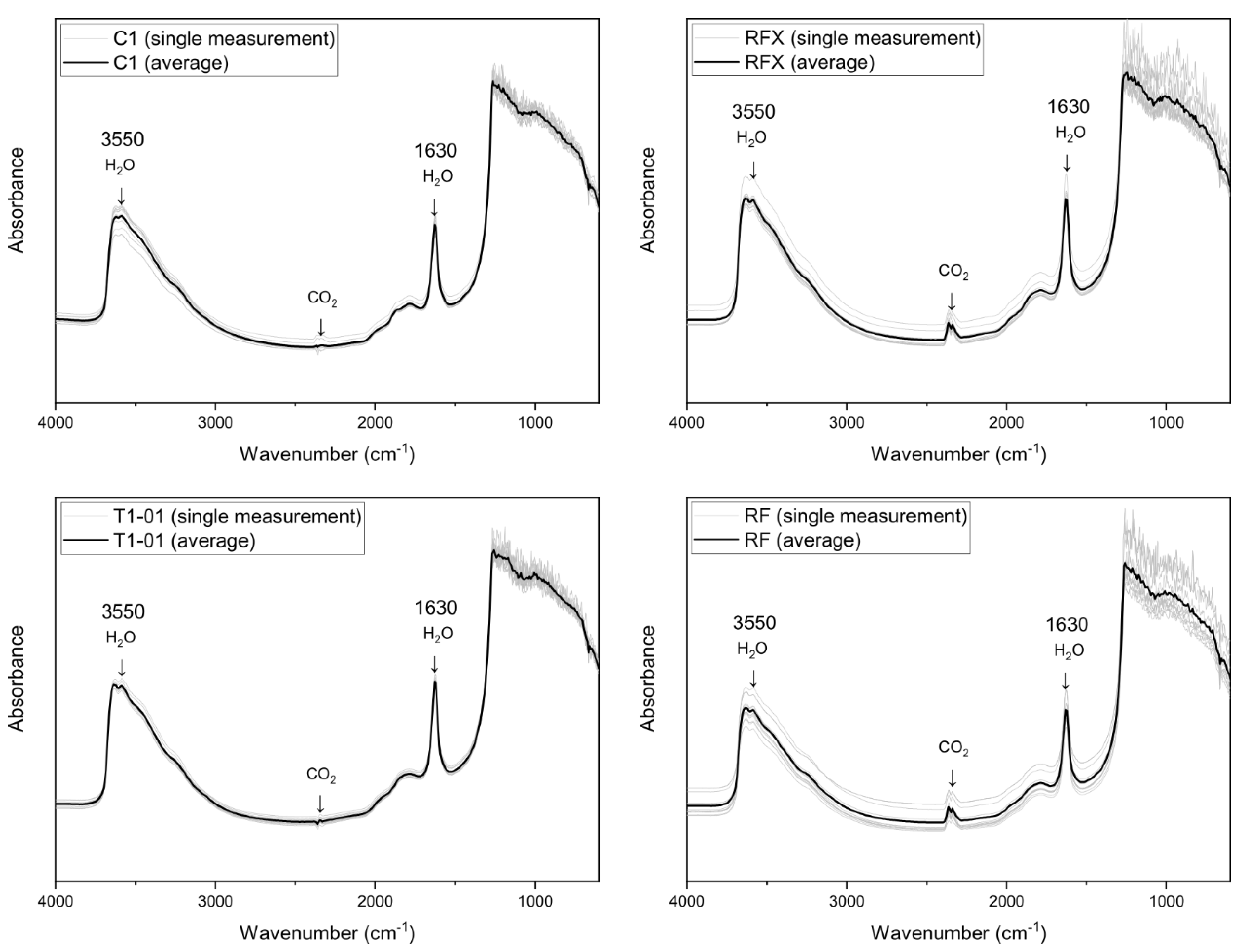
Appendix A.2. FTIR-Analysis


Appendix A.3. Point Counting (Crystal Content)
| Samples | Total Points Counted | Crystal Content (%) |
|---|---|---|
| Great Dyke | ||
| M1 | 333 | 29.4 |
| C1 | 286 | 30.1 |
| Sosa Dyke | ||
| T1-01 | 336 | 36.9 |
| T1-02 | 320 | 35.0 |
| T1-05 | 310 | 35.5 |
| T1-09 | 312 | 37.5 |
| T2-03 | 322 | 39.1 |
| T2-06 | 293 | 35.5 |
Appendix B. Characterisation of AMS Carriers in the Sosa Dyke Rocks


Appendix C. Data Figure 9
| Segment | rtip (m) | w (m) | t (m) | rtip/w | t/w |
|---|---|---|---|---|---|
| Sosa Dyke | |||||
| SI3 | 25.34 | 560 | 51 | 0.02 | 0.09 |
| SII | 17.47 | 210 | 61 | 0.04 | 0.29 |
| SIII | 64.17 | 203 | 74 | 0.16 | 0.36 |
| Great Dyke | |||||
| Segment1 | 3.10 | 78 | 27 | 0.04 | 0.35 |
| Segment1 | 7.00 | 78 | 27 | 0.09 | 0.35 |
| Segment2 | 9.09 | 45 | 23 | 0.20 | 0.51 |
| Segment2 | 8.67 | 45 | 23 | 0.19 | 0.51 |
| Segment3 | 7.75 | 95 | 25 | 0.08 | 0.26 |
| Segment3 | 11.42 | 95 | 25 | 0.12 | 0.26 |
| Segment4 | 10.42 | 145 | 29 | 0.07 | 0.20 |
| Segment4 | 8.83 | 145 | 29 | 0.06 | 0.20 |
| Segment5 | 12.51 | 158 | 32 | 0.08 | 0.20 |
| Segment5 | 13.09 | 158 | 32 | 0.08 | 0.20 |
| Segment6 | 14.08 | 93 | 40 | 0.15 | 0.43 |
| Segment6 | 14.42 | 93 | 40 | 0.16 | 0.43 |
| Segment7 | 10.25 | 1110 | 36 | 0.01 | 0.03 |
| Segment7 | 10.68 | 1110 | 36 | 0.01 | 0.03 |
| Segment8 | 5.58 | 220 | 21 | 0.03 | 0.10 |
| Segment8 | 1.61 | 220 | 21 | 0.01 | 0.10 |
References
- Kavanagh, J.L. Chapter 3—Mechanisms of Magma Transport in the Upper Crust—Dyking. In Volcanic and Igneous Plumbing Systems Understanding Magma Transport, Storage, and Evolution in the Earth’s Crust; Burchardt, S., Ed.; Elsevier: Amsterdam, The Netherlands, 2018; pp. 55–88. ISBN 978-0-12-809749-6. [Google Scholar]
- Cruden, A.R.; McCaffrey, K.J.W.; Bunger, A.P. Geometric Scaling of Tabular Igneous Intrusions: Implications for Emplacement and Growth. In Physical Geology of Shallow Magmatic Systems: Dykes, Sills and Laccoliths; Breitkreuz, C., Rocchi, S., Eds.; Springer International Publishing: Cham, Switzerland, 2018; pp. 11–38. ISBN 978-3-319-14084-1. [Google Scholar]
- Galland, O.; Bertelsen, H.S.; Eide, C.H.; Guldstrand, F.; Haug, Ø.T.; Leanza, H.A.; Mair, K.; Palma, O.; Planke, S.; Rabbel, O.; et al. Storage and Transport of Magma in the Layered Crust-Formation of Sills and Related Flat-Lying Intrusions. In Volcanic and Igneous Plumbing Systems; Burchardt, S., Ed.; Elsevier: Amsterdam, The Netherlands, 2018; pp. 111–136. ISBN 9780128097496. [Google Scholar]
- Sigmundsson, F. New insights into magma plumbing along rift systems from detailed observations of eruptive behavior at Axial volcano. Geophys. Res. Lett. 2016, 43, 12.423–12.427. [Google Scholar] [CrossRef]
- Chen, K.; Smith, J.D.; Avouac, J.-P.; Liu, Z.; Song, Y.T.; Gualandi, A. Triggering of the Mw 7.2 Hawaii Earthquake of 4 May 2018 by a Dike Intrusion. Geophys. Res. Lett. 2019, 46, 2503–2510. [Google Scholar] [CrossRef]
- Wicks, C.; de la Llera, J.C.; Lara, L.E.; Lowenstern, J. The role of dyking and fault control in the rapid onset of eruption at Chaitén volcano, Chile. Nature 2011, 478, 374–377. [Google Scholar] [CrossRef] [PubMed]
- Fahrig, W.F.; Halls, H.C. Mafic Dyke Swarms; Geological Association of Canada: Toronto, ON, Canada, 1987; p. 503. [Google Scholar]
- Kjøll, H.J.; Galland, O.; Labrousse, L.; Andersen, T.B. Emplacement mechanisms of a dyke swarm across the brittle-ductile transition and the geodynamic implications for magma-rich margins. Earth Planet. Sci. Lett. 2019, 518, 223–235. [Google Scholar] [CrossRef]
- Melnik, O.; Barmin, A.A.; Sparks, R.S.J. Dynamics of magma flow inside volcanic conduits with bubble overpressure buildup and gas loss through permeable magma. J. Volcanol. Geotherm. Res. 2005, 143, 53–68. [Google Scholar] [CrossRef]
- Michaut, C.; Ricard, Y.; Bercovici, D.; Sparks, R.S.J. Eruption cyclicity at silicic volcanoes potentially caused by magmatic gas waves. Nat. Geosci. 2013, 6, 856–860. [Google Scholar] [CrossRef]
- Emerman, S.H.; Marrett, R. Why dikes? Geology 1990, 18, 231–233. [Google Scholar] [CrossRef]
- Burchardt, S. Volcanic and Igneous Plumbing Systems: Understanding Magma Transport, Storage, and Evolution in the Earth’s Crust; Elsevier: Amsterdam, The Netherlands, 2018; ISBN 9780128097496. [Google Scholar]
- Rocchi, S.; Breitkreuz, C. Physical Geology of Shallow-Level Magmatic Systems—An Introduction. In Physical Geology of Shallow Magmatic Systems: Dykes, Sills and Laccoliths; Breitkreuz, C., Rocchi, S., Eds.; Springer International Publishing: Cham, Germany, 2017; pp. 1–10. ISBN 978-3-319-14084-1. [Google Scholar]
- Jay, J.; Costa, F.; Pritchard, M.; Lara, L.; Singer, B.; Herrin, J. Locating magma reservoirs using InSAR and petrology before and during the 2011–2012 Cordón Caulle silicic eruption. Earth Planet. Sci. Lett. 2014, 395, 254–266. [Google Scholar] [CrossRef]
- Heiken, G.; Wohletz, K.; Eichelberger, J. Fracture fillings and intrusive pyroclasts, Inyo Domes, California. J. Geophys. Res. Solid Earth 1988, 93, 4335–4350. [Google Scholar] [CrossRef]
- Eichelberger, J.C.; Carrigan, C.R.; Westrich, H.R.; Price, R.H. Non-explosive silicic volcanism. Nature 1986, 323, 598–602. [Google Scholar] [CrossRef]
- Watkins, H.; Healy, D.; Bond, C.E.; Butler, R.W.H. Implications of heterogeneous fracture distribution on reservoir quality; an analogue from the Torridon Group sandstone, Moine Thrust Belt, NW Scotland. J. Struct. Geol. 2018, 108, 180–197. [Google Scholar] [CrossRef]
- Healy, D.; Rizzo, R.; Duffy, M.; Farrell, N.; Hole, M.; Muirhead, D. Field evidence for the lateral emplacement of igneous dykes: Implications for 3D mechanical models and the plumbing beneath fissure eruptions. Volcanica 2018, 1, 85–105. [Google Scholar] [CrossRef]
- Rubin, A.M. Propagation of Magma-Filled Cracks. Annu. Rev. Earth Planet. Sci. 1995, 23, 287–336. [Google Scholar] [CrossRef]
- Rivalta, E.; Taisne, B.; Bunger, A.P.; Katz, R.F. A review of mechanical models of dike propagation: Schools of thought, results and future directions. Tectonophysics 2015, 638, 1–42. [Google Scholar] [CrossRef]
- Poppe, S.; Galland, O.; de Winter, N.J.; Goderis, S.; Claeys, P.; Debaille, V.; Boulvais, P.; Kervyn, M. Structural and Geochemical Interactions Between Magma and Sedimentary Host Rock: The Hovedøya Case, Oslo Rift, Norway. Geochem. Geophys. Geosystems 2020, 21, e2019GC008685. [Google Scholar] [CrossRef]
- Rubin, A.M. On the thermal viability of dikes leaving magma chambers. Geophys. Res. Lett. 1993, 20, 257–260. [Google Scholar] [CrossRef]
- Burchardt, S.; Tanner, D.C.; Troll, V.R.; Krumbholz, M.; Gustafsson, L.E. Three-dimensional geometry of concentric intrusive sheet swarms in the Geitafell and the Dyrfjöll volcanoes, eastern Iceland. Geochem. Geophys. Geosystems 2011, 12, Q0AB09. [Google Scholar] [CrossRef]
- Daniels, K.A.; Kavanagh, J.L.; Menand, T.; Stephen, J.S.R. The shapes of dikes: Evidence for the influence of cooling and inelastic deformation. GSA Bull. 2012, 124, 1102–1112. [Google Scholar] [CrossRef]
- Pollard, D.D.; Muller, O.H.; Dockstader, D.R. The Form and Growth of Fingered Sheet Intrusions. Geol. Soc. Am. Bull. 1975, 86, 351–363. [Google Scholar] [CrossRef]
- Spacapan, J.B.; Galland, O.; Leanza, H.A.; Planke, S. Igneous sill and finger emplacement mechanism in shale-dominated formations: A field study at Cuesta del Chihuido, Neuquén Basin, Argentina. J. Geol. Soc. Lon. 2017, 174, 422–433. [Google Scholar] [CrossRef]
- Galland, O.; Spacapan, J.B.; Rabbel, O.; Mair, K.; Soto, F.G.; Eiken, T.; Schiuma, M.; Leanza, H.A.; Spacapan, J.B.; Soto, F.G.; et al. Structure, emplacement mechanism and magma-flow significance of igneous fingers – Implications for sill emplacement in sedimentary basins. J. Struct. Geol. 2019, 124, 120–135. [Google Scholar] [CrossRef]
- Stephens, T.L.; Walker, R.J.; Healy, D.; Bubeck, A. Segment tip geometry of sheet intrusions, II: Field observations of tip geometries and a model for evolving emplacement mechanisms. EarthARXiv 2020. Available online: https://eartharxiv.org/repository/view/1794/ (accessed on 10 October 2021). [CrossRef]
- Schofield, N.; Stevenson, C.; Reston, T. Magma fingers and host rock fluidization in the emplacement of sills. Geology 2010, 38, 63–66. [Google Scholar] [CrossRef]
- Schmiedel, T.; Galland, O.; Breitkreuz, C. Dynamics of Sill and Laccolith Emplacement in the Brittle Crust: Role of Host Rock Strength and Deformation Mode. J. Geophys. Res. Solid Earth 2017, 122, 8860–8871. [Google Scholar] [CrossRef]
- Schofield, N.; Brown, D.J.; Magee, C.; Stevenson, C.T. Sill morphology and comparison of brittle and non-brittle emplacement mechanisms. J. Geol. Soc. Lond. 2012, 169, 127–141. [Google Scholar] [CrossRef]
- Bertelsen, H.; Rogers, B.; Galland, O.; Dumazer, G.; Benanni, A. Laboratory modeling of coeval brittle and ductile deformation during magma emplacement into viscoelastic rocks. Front. Earth Sci. 2018, 6, 1–16. [Google Scholar] [CrossRef]
- Knight, M.D.; Walker, G.P.L. Magma flow directions in dikes of the Koolau complex, Oahu, determined from magnetic fabric studies (Hawaii). J. Geophys. Res. Solid Earth 1988, 93, 4301–4319. [Google Scholar] [CrossRef]
- Tauxe, L.; Gee, J.S.; Staudigel, H. Flow directions in dikes from anisotropy of magnetic susceptibility data: The bootstrap way. J. Geophys. Res. Solid Earth 1998, 103, 17775–17790. [Google Scholar] [CrossRef]
- Poland, M.P.; Fink, J.H.; Tauxe, L. Patterns of magma flow in segmented silicic dikes at Summer Coon volcano, Colorado: AMS and thin section analysis. Earth Planet. Sci. Lett. 2004, 219, 155–169. [Google Scholar] [CrossRef]
- Abdelmalak, M.M.; Mourgues, R.; Galland, O.; Bureau, D. Fracture mode analysis and related surface deformation during dyke intrusion: Results from 2D experimental modelling. Earth Planet. Sci. Lett. 2012, 359–360, 93–105. [Google Scholar] [CrossRef]
- Guldstrand, F.; Burchardt, S.; Hallot, E.; Galland, O. Dynamics of Surface Deformation Induced by Dikes and Cone Sheets in a Cohesive Coulomb Brittle Crust. J. Geophys. Res. Solid Earth 2017, 122, 8511–8524. [Google Scholar] [CrossRef]
- Castro, J.M.; Dingwell, D.B. Rapid ascent of rhyolitic magma at Chaitén volcano, Chile. Nature 2009, 461, 780–783. [Google Scholar] [CrossRef] [PubMed]
- Castro, J.M.; Schipper, C.I.; Mueller, S.P.; Militzer, A.S.; Amigo, A.; Parejas, C.S.; Jacob, D. Storage and eruption of near-liquidus rhyolite magma at Cordón Caulle, Chile. Bull. Volcanol. 2013, 75, 702. [Google Scholar] [CrossRef]
- Bertelsen, H.S.; Guldstrand, F.; Sigmundsson, F.; Pedersen, R.; Mair, K.; Galland, O. Beyond elasticity: Are Coulomb properties of the Earth’s crust important for volcano geodesy? J. Volcanol. Geotherm. Res. 2021, 410, 107153. [Google Scholar] [CrossRef]
- Burchardt, S. Chapter 12—Synthesis on the State-of-the-Art and Future Directions in the Research on Volcanic and Igneous Plumbing Systems. In Volcanic and Igneous Plumbing Systems Understanding Magma Transport, Storage, and Evolution in the Earth’s Crust; Burchardt, S., Ed.; Elsevier: Amsterdam, The Netherlands, 2018; pp. 323–333. ISBN 978-0-12-809749-6. [Google Scholar]
- Magee, C.; Stevenson, C.T.E.; Ebmeier, S.K.; Keir, D.; Hammond, J.O.S.; Gottsmann, J.H.; Whaler, K.A.; Schofield, N.; Jackson, C.A.L.; Petronis, M.S.; et al. Magma plumbing systems: A geophysical perspective. J. Petrol. 2018, 59, 1217–1251. [Google Scholar] [CrossRef]
- Llambías, E.J.; Bertotto, G.W.; Risso, C.; Hernando, I. El volcanismo cuaternario en el retroarco de Payenia: Una revisión. Rev. la Asoc. Geol. Argentina 2010, 67, 278–300. [Google Scholar]
- Folguera, A.; Ramos, V.A. Repeated eastward shifts of arc magmatism in the Southern Andes: A revision to the long-term pattern of Andean uplift and magmatism. J. South Am. Earth Sci. 2011, 32, 531–546. [Google Scholar] [CrossRef]
- Kay, S.M.; Mancilla, O.; Copeland, P. Evolution of the late Miocene Chachahuén volcanic complex at 37°S over a transient shallow subduction zone under the Neuquén Andes. Geol. Soc. Am. Spec. Pap. 2006, 407, 215–246. [Google Scholar] [CrossRef]
- Holmberg, E. Descripción Geológica de la Hoja 32 d, Chachahuén. Provincia del Neuquén - Provincia de Mendoza. Escala 1:200.000. Carta Geológico-Económica de la República Argentina. Boletines del SEGEMAR 1962, 91, 70. [Google Scholar]
- González Díaz, E.F. Descripción Geológica de la Hoja 31 d, La Matancilla. Provincia de Mendoza. Escala 1:200.000. Carta Geológico-Económica de la República Argentina. Boletines del SEGEMAR 1979, 173, 97. [Google Scholar]
- Perez, M.A.; Condat, P. Geología de la Sierra de Chachahuén, Á rea CNQ-23; Puelen: Buenos Aires, Argentina, 1996. [Google Scholar]
- Burchardt, S.; Mattsson, T.; Palma, J.O.; Galland, O.; Almqvist, B.; Mair, K.; Jerram, D.A.; Hammer, Ø.; Sun, Y. Progressive Growth of the Cerro Bayo Cryptodome, Chachahuén Volcano, Argentina—Implications for Viscous Magma Emplacement. J. Geophys. Res. Solid Earth 2019, 124, 7934–7961. [Google Scholar] [CrossRef]
- Sagripanti, L.; Aguirre-Urreta, B.; Folguera, A.; Ramos, V.A. The Neocomian of Chachahuén (Mendoza, Argentina): Evidence of a broken foreland associated with the Payenia flat-slab. Geol. Soc. Lond. Spec. Publ. 2015, 399, 203–219. [Google Scholar] [CrossRef]
- Guldstrand, F.; Schmiedel, T. 2021. Available online: https://zenodo.org/record/4784165/export/hx#.YWP33xpByUk (accessed on 4 October 2021).
- Jelínek, V. Statistical processing of anisotropy of magnetic susceptibility measured on groups of specimens. Stud. Geophys. Geod. 1978, 22, 50–62. [Google Scholar] [CrossRef]
- Khan, M.A. The anisotropy of magnetic susceptibility of some igneous and metamorphic rocks. J. Geophys. Res. 1962, 67, 2873–2885. [Google Scholar] [CrossRef]
- Jelinek, V. Characterization of the magnetic fabric of rocks. Tectonophysics 1981, 79, T34–T67. [Google Scholar] [CrossRef]
- Chadima, M.; Hrouda, F.; Jelínek, V. Anisoft5; AGICO: Brno, Czech Republic, 2020. [Google Scholar]
- Hrouda, F.; Chadima, M.; Ježek, J.; Pokorný, J. Anisotropy of out-of-phase magnetic susceptibility of rocks as a tool for direct determination of magnetic subfabrics of some minerals: An introductory study. Geophys. J. Int. 2017, 208, 385–402. [Google Scholar] [CrossRef]
- Hrouda, F.; Ježek, J.; Chadima, M. Anisotropy of out-of-phase magnetic susceptibility as a potential tool for distinguishing geologically and physically controlled inverse magnetic fabrics in volcanic dykes. Phys. Earth Planet. Inter. 2020, 307, 106551. [Google Scholar] [CrossRef]
- Hext, G.R. The estimation of second-order tensors, with related tests and designs. Biometrika 1963, 50, 353–373. [Google Scholar] [CrossRef]
- Jelínek, V. The Statistical Theory of Measuring Anisotropy of Magnetic Susceptibility of Rocks and Its Application; Geofyzika: Brno, Czech Republic, 1977. [Google Scholar]
- Jackson, L.L.; Brown, F.W.; Neil, S.T. Major and minor elements requiring individual determination, classical whole rock analysis, and rapid rock analysis. US Geol. Surv. Bull. 1987, 1770, G1–G23. [Google Scholar]
- von Aulock, F.W.; Kennedy, B.M.; Schipper, C.I.; Castro, J.M.E.; Martin, D.; Oze, C.; Watkins, J.M.; Wallace, P.J.; Puskar, L.; Bégué, F.; et al. Advances in Fourier transform infrared spectroscopy of natural glasses: From sample preparation to data analysis. Lithos 2014, 206–207, 52–64. [Google Scholar] [CrossRef]
- McIntosh, I.M.; Llewellin, E.W.; Humphreys, M.C.S.; Nichols, A.R.L.; Burgisser, A.; Schipper, C.I.; Larsen, J.F. Distribution of dissolved water in magmatic glass records growth and resorption of bubbles. Earth Planet. Sci. Lett. 2014, 401, 1–11. [Google Scholar] [CrossRef]
- McIntosh, I.M.; Nichols, A.R.L.; Tani, K.; Llewellin, E.W. Accounting for the species-dependence of the 3500 cm-1 H2Ot infrared molar absorptivity coefficient: Implications for hydrated volcanic glasses. Am. Mineral. 2017, 102, 1677–1689. [Google Scholar] [CrossRef]
- Bottinga, Y.; Weill, D.F. The viscosity of magmatic silicate liquids; a model calculation. Am. J. Sci. 1972, 272, 438–475. [Google Scholar] [CrossRef]
- Lamé, G. Examen des Différentes Méthodes Employées Pour Résoudre les Problémes de Géométrie; M V Courcier: Paris, France, 1818. [Google Scholar]
- Walker, R.; Stephens, T.L.; Greenfield, C.; Gill, S.; Healy, D.; Poppe, S. Segment tip geometry of sheet intrusions, I: Theory and numerical models for the role of tip shape in controlling propagation pathways. EarthArXiv 2021. Available online: https://eartharxiv.org/ (accessed on 10 October 2021). [CrossRef]
- Hargraves, R.B.; Johnson, D.; Chan, C.Y. Distribution anisotropy: The cause of AMS in igneous rocks? Geophys. Res. Lett. 1991, 18, 2193–2196. [Google Scholar] [CrossRef]
- Stephenson, A. Distribution anisotropy: Two simple models for magnetic lineation and foliation. Phys. Earth Planet. Inter. 1994, 82, 49–53. [Google Scholar] [CrossRef]
- Cañón-Tapia, E. Factors affecting the relative importance of shape and distribution anisotropy in rocks: Theory and experiments. Tectonophysics 2001, 340, 117–131. [Google Scholar] [CrossRef]
- Borradaile, G.J.G.J.; Jackson, M. Structural geology, petrofabrics and magnetic fabrics (AMS, AARM, AIRM). J. Struct. Geol. 2010, 32, 1519–1551. [Google Scholar] [CrossRef]
- Mattsson, T.; Petri, B.; Almqvist, B.S.G.; McCarthy, W.; Burchardt, S.; Palma, J.O.; Hammer, Ø.; Galland, O. Decrypting magnetic fabrics (AMS, AARM, AIRM) through the analysis of mineral shape fabrics and distribution anisotropy. J. Geophys. Res. Solid Earth 2021, 126, e2021JB021895. [Google Scholar] [CrossRef]
- Browne, B.L.; Gardner, J.E. The influence of magma ascent path on the texture, mineralogy, and formation of hornblende reaction rims. Earth Planet. Sci. Lett. 2006, 246, 161–176. [Google Scholar] [CrossRef]
- Huppert, H.E.; Sparks, R.S.J. Chilled margins in igneous rocks. Earth Planet. Sci. Lett. 1989, 92, 397–405. [Google Scholar] [CrossRef]
- Schmiedel, T.; Kjoberg, S.; Planke, S.; Magee, C.; Galland, O.; Schofield, N.; Jackson, C.A.-L.; Jerram, D.A. Mechanisms of overburden deformation associated with the emplacement of the Tulipan sill, mid-Norwegian margin. Interpretation 2017, 5, SK23–SK38. [Google Scholar] [CrossRef]
- Köpping, J.; Magee, C.; Cruden, A.R.; Jackson, C.A.-L.; Norcliffe, J. The building blocks of igneous sheet intrusions: Insights from 3D seismic reflection data. EarthArXiv 2021. [Google Scholar] [CrossRef]
- Eide, C.H.; Schofield, N.; Lecomte, I.; Buckley, S.J.; Howell, J.A. Seismic interpretation of sill complexes in sedimentary basins: Implications for the sub-sill imaging problem. J. Geol. Soc. Lond. 2018, 175, 193–209. [Google Scholar] [CrossRef]
- Wiebe, R.A.; Ulrich, R. Origin of composite dikes in the Gouldsboro granite, coastal Maine. Lithos 1997, 40, 157–178. [Google Scholar] [CrossRef]
- Eriksson, P.I.; Riishuus, M.S.; Sigmundsson, F.; Elming, S.-Å.Å. Magma flow directions inferred from field evidence and magnetic fabric studies of the Streitishvarf composite dike in east Iceland. J. Volcanol. Geotherm. Res. 2011, 206, 30–45. [Google Scholar] [CrossRef]
- Carrigan, C.R.; Eichelberger, J.C. Zoning of magmas by viscosity in volcanic conduits. Nature 1990, 343, 248–251. [Google Scholar] [CrossRef]
- Geoffroy, L.; Callot, J.P.; Aubourg, C.; Moreira, M. Magnetic and plagioclase linear fabric discrepancy in dykes: A new way to define the flow vector using magnetic foliation. Terra Nov. 2002, 14, 183–190. [Google Scholar] [CrossRef]
- Chadima, M.; Cajz, V.; Týcová, P. On the interpretation of normal and inverse magnetic fabric in dikes: Examples from the Eger Graben, NW Bohemian Massif. Tectonophysics 2009, 466, 47–63. [Google Scholar] [CrossRef]
- Andersson, M.; Almqvist, B.S.G.; Burchardt, S.; Troll, V.R.; Malehmir, A.; Snowball, I.; Kübler, L. Magma transport in sheet intrusions of the Alnö carbonatite complex, central Sweden. Sci. Rep. 2016, 6, 27635. [Google Scholar] [CrossRef]
- Magee, C.; Muirhead, J.D.; Karvelas, A.; Holford, S.P.; Jackson, C.A.L.; Bastow, I.D.; Schofield, N.; Stevenson, C.T.E.; McLean, C.; McCarthy, W. Lateral magma flow in mafic sill complexes. Geosphere 2016, 12, 809–841. [Google Scholar] [CrossRef]
- Hutton, D.H.W. Insights into magmatism in volcanic margins: Bridge structures and a new mechanism of basic sill emplacement–Theron Mountains, Antarctica. Pet. Geosci. 2009, 15, 269–278. [Google Scholar] [CrossRef]
- Magee, C.; Muirhead, J.; Schofield, N.; Walker, R.J.; Galland, O.; Holford, S.; Spacapan, J.; Jackson, C.A.-L.; McCarthy, W. Structural signatures of igneous sheet intrusion propagation. J. Struct. Geol. 2019, 125, 148–154. [Google Scholar] [CrossRef]
- Delaney, P.T.; Pollard, D.D. United States Government Printing Office. Deformation of Host Rocks and Flow of Magma during Growth of Minette Dikes and Breccia-Bearing Intrusions near Ship Rock, New Mexico; United States Government Printing Office: Washington, DC, USA, 1981. [Google Scholar]
- Kjoberg, S.; Schmiedel, T.; Planke, S.; Svensen, H.H.; Millett, J.M.; Jerram, D.A.; Galland, O.; Lecomte, I.; Schofield, N.; Haug, Ø.T.; et al. 3D structure and formation of hydrothermal vent complexes at the Paleocene-Eocene transition, the Møre Basin, mid-Norwegian margin. Interpretation 2017, 5, SK65–SK81. [Google Scholar] [CrossRef]
- Arachchige, U.N.; Cruden, A.R.; Weinberg, R. Laponite gels - visco-elasto-plastic analogues for geological laboratory modelling. Tectonophysics 2021, 805, 228773. [Google Scholar] [CrossRef]
- Kavanagh, J.L.; Engwell, S.L.; Martin, S.A. A review of laboratory and numerical modelling in volcanology. Solid Earth 2018, 9, 531–571. [Google Scholar] [CrossRef]
- Townsend, M.R.; Pollard, D.D.; Smith, R.P. Mechanical models for dikes: A third school of thought. Tectonophysics 2017, 703, 98–118. [Google Scholar] [CrossRef]
- Vachon, R.; Bazargan, M.; Hieronymus, C.F.; Ronchin, E.; Almqvist, B. Crystal rotations and alignment in spatially varying magma flows: 2-D examples of common subvolcanic flow geometries. Geophys. J. Int. 2021, 226, 709–727. [Google Scholar] [CrossRef]
- Poland, M.P.; Moats, W.P.; Fink, J.H. A model for radial dike emplacement in composite cones based on observations from Summer Coon volcano, Colorado, USA. Bull. Volcanol. 2008, 70, 861–875. [Google Scholar] [CrossRef]
- Takeuchi, S. Preeruptive magma viscosity: An important measure of magma eruptibility. J. Geophys. Res. Solid Earth 2011, 116, 19. [Google Scholar] [CrossRef]
- Richet, P.; Lejeune, A.-M.; Holtz, F.; Roux, J. Water and the viscosity of andesite melts. Chem. Geol. 1996, 128, 185–197. [Google Scholar] [CrossRef]
- Heap, M.J.; Violay, M.E.S. The mechanical behaviour and failure modes of volcanic rocks: A review. Bull. Volcanol. 2021, 83, 47. [Google Scholar] [CrossRef]
- Eide, C.H.; Schofield, N.; Jerram, D.A.; Howell, J.A. Basin-scale architecture of deeply emplaced sill complexes: Jameson Land, East Greenland. J. Geol. Soc. Lond. 2016, 174, 23–40. [Google Scholar] [CrossRef]
- Haug, Ø.T.; Galland, O.; Souloumiac, P.; Souche, A.; Guldstrand, F.; Schmiedel, T. Inelastic damage as a mechanical precursor for the emplacement of saucer-shaped intrusions. Geology 2017, 45, 1099–1102. [Google Scholar] [CrossRef]
- Schmiedel, T.; Galland, O.; Haug, Ø.T.; Dumazer, G.; Breitkreuz, C. Coulomb failure of Earth’s brittle crust controls growth, emplacement and shapes of igneous sills, saucer-shaped sills and laccoliths. Earth Planet. Sci. Lett. 2019, 510, 161–172. [Google Scholar] [CrossRef]
- Galland, O.; Burchardt, S.; Hallot, E.; Mourgues, R.; Bulois, C. Dynamics of dikes versus cone sheets in volcanic systems. J. Geophys. Res. Solid Earth 2014, 119, 6178–6192. [Google Scholar] [CrossRef]
- Galland, O.; Schmiedel, T.; Bertelsen, H.; Guldstrand, F.; Haug, Ø.T.; Souche, A. Geomechanical Modeling of Fracturing and Damage induced by Igneous Intrusions: Implications for Fluid Flow in Volcanic Basins. In Proceedings of the X Congreso de Exploración y Desarrollo de Hidrocarburos, Mendoza, Argentina, 5–9 November 2018; Instituto Argentino del Petróleo y el Gas: Mendoza, Argentina, 2018; pp. 1–16. [Google Scholar]
- Vachon, R.; Hieronymus, C.F. Effect of host-rock rheology on dyke shape, thickness and magma overpressure. Geophys. J. Int. 2017, 208, 1414–1429. [Google Scholar] [CrossRef][Green Version]
- Souche, A.; Galland, O.; Haug, Ø.T.; Dabrowski, M. Impact of host rock heterogeneity on failure around pressurized conduits: Implications for finger-shaped magmatic intrusions. Tectonophysics 2019, 765, 52–63. [Google Scholar] [CrossRef]
- Gudmundsson, A.; Loetveit, I.F. Dyke emplacement in a layered and faulted rift zone. J. Volcanol. Geotherm. Res. 2005, 144, 311–327. [Google Scholar] [CrossRef]
- Perras, M.A.; Diederichs, M.S. A Review of the Tensile Strength of Rock: Concepts and Testing. Geotech. Geol. Eng. 2014, 32, 525–546. [Google Scholar] [CrossRef]
- Petford, N.; Cruden, A.R.; McCaffrey, K.J.W.; Vigneresse, J.L. Granite magma formation, transport and emplacement in the Earth’s crust. Nature 2000, 408, 669–673. [Google Scholar] [CrossRef] [PubMed]
- Scaillet, B.; Holtz, F.; Pichavant, M. Phase equilibrium constraints on the viscosity of silicic magmas: 1. Volcanic-plutonic comparison. J. Geophys. Res. Solid Earth 1998, 103, 27257–27266. [Google Scholar] [CrossRef]
- Pollard, D.D. Derivation and evaluation of a mechanical model for sheet intrusions. Tectonophysics 1973, 19, 233–269. [Google Scholar] [CrossRef]
- Scheibert, J.; Galland, O.; Hafver, A. Inelastic deformation during sill and laccolith emplacement: Insights from an analytic elastoplastic model. J. Geophys. Res. Solid Earth 2017, 122, 923–945. [Google Scholar] [CrossRef]
- Rivas-Dorado, S.; Ruiz, J.; Romeo, I. Subsurface Geometry and Emplacement Conditions of a Giant Dike System in Elysium Fossae, Mars. J. Geophys. Res. Planets 2021, 126, e2020JE006512. [Google Scholar] [CrossRef]
- Lattard, D.; Engelmann, R.; Kontny, A.; Sauerzapf, U. Curie temperatures of synthetic titanomagnetites in the Fe-Ti-O system: Effects of composition, crystal chemistry, and thermomagnetic methods. J. Geophys. Res. Solid Earth 2006, 111, B12S28. [Google Scholar] [CrossRef]
- Petronis, M.S.; O’Driscoll, B.; Lindline, J. Late stage oxide growth associated with hydrothermal alteration of the Western Granite, Isle of Rum, NW Scotland. Geochem. Geophys. Geosyst. 2011, 12, 1–32. [Google Scholar] [CrossRef]
- Dunlop, D.J.; Özdemir, Ö. Rock Magnetism. Fundamentals and Frontiers; Cambridge University Press: Cambridge, NY, USA, 1997; Volume 135. [Google Scholar]
- Kontny, A.; Grothaus, L. Effects of shock pressure and temperature on titanomagnetite from ICDP cores and target rocks of the El’gygytgyn impact structure, Russia. Stud. Geophys. Geod. 2017, 61, 162–183. [Google Scholar] [CrossRef]
- Bilardello, D. Practical Magnetism II: Humps and a Bump, the Maghemite Song The IRM Quarterly. IRM Q. 2020, 30, 1–17. [Google Scholar]
- McCabe, C.; Jackson, M.; Ellwood, B.B. Magnetic anisotropy in the Trenton Limestone: Results of a new technique, anisotropy of anhysteretic susceptibility. Geophys. Res. Lett. 1985, 12, 333–336. [Google Scholar] [CrossRef]
- Jackson, M. Anisotropy of magnetic remanence: A brief review of mineralogical sources, physical origins, and geological applications, and comparison with susceptibility anisotropy. Pure Appl. Geophys. PAGEOPH 1991, 136, 1–28. [Google Scholar] [CrossRef]
- Bilardello, D.; Jackson, M.J. A comparative study of magnetic anisotropy measurement techniques in relation to rock-magnetic properties. Tectonophysics 2014, 629, 39–54. [Google Scholar] [CrossRef]
- Tarling, D.; Hrouda, F. Magnetic Anisotropy of Rocks, 1st ed.; Springer: Amsterdam, The Netherlands, 1993. [Google Scholar]
- Bogue, S.W.; Gromme, S.; Hillhouse, J.W. Paleomagnetism, magnetic anisotropy, and mid-Cretaceous paleolatitude of the Duke Island (Alaska) ultramafic complex. Tectonics 1995, 14, 1133–1152. [Google Scholar] [CrossRef]
- Stephenson, A.; Sadikun, S.; Potter, D.K. A theoretical and experimental comparison of the anisotropies of magnetic susceptibility and remanence in rocks and minerals. Geophys. J. Int. 1986, 84, 185–200. [Google Scholar] [CrossRef]
- Lagroix, F.; Borradaile, G.J. Magnetic fabric interpretation complicated by inclusions in mafic silicates. Tectonophysics 2000, 325, 207–225. [Google Scholar] [CrossRef]
- Selkin, P.A.; Gee, J.S.; Meurer, W.P. Magnetic anisotropy as a tracer of crystal accumulation and transport, Middle Banded Series, Stillwater Complex, Montana. Tectonophysics 2014, 629, 123–137. [Google Scholar] [CrossRef]
- Renne, P.R.; Scott, G.R.; Glen, J.M.G.; Feinberg, J.M. Oriented inclusions of magnetite in clinopyroxene: Source of stable remanent magnetization in gabbros of the Messum Complex, Namibia. Geochem. Geophys. Geosyst. 2002, 3, 1–11. [Google Scholar] [CrossRef]


| Input Parameters | ||||
|---|---|---|---|---|
| Major element geochemistry | See Table A1 and Table A2 | |||
| Total water content/FTIR spectroscopy (wt%) | Great Dyke | Sosa Dyke | ||
| 1.50 | 1.49 | |||
| Crystal content (%) | 30–38 | 29–39 | ||
| Average crystal/vesicle size (mm) | 1.0 | 1.5 | ||
| Pressure (MPa) 1 | 10 | |||
| Temperature (°C) 1 | 790 | 850 | 790 | 850 |
| Results | ||||
| Average effective viscosity ηeff (Pa·s) | 2.42 × 10⁶ | 1.17 × 10⁶ | 5.20 × 10⁶ | 2.54 × 10⁶ |
Publisher’s Note: MDPI stays neutral with regard to jurisdictional claims in published maps and institutional affiliations. |
© 2021 by the authors. Licensee MDPI, Basel, Switzerland. This article is an open access article distributed under the terms and conditions of the Creative Commons Attribution (CC BY) license (https://creativecommons.org/licenses/by/4.0/).
Share and Cite
Schmiedel, T.; Burchardt, S.; Mattsson, T.; Guldstrand, F.; Galland, O.; Palma, J.O.; Skogby, H. Emplacement and Segment Geometry of Large, High-Viscosity Magmatic Sheets. Minerals 2021, 11, 1113. https://doi.org/10.3390/min11101113
Schmiedel T, Burchardt S, Mattsson T, Guldstrand F, Galland O, Palma JO, Skogby H. Emplacement and Segment Geometry of Large, High-Viscosity Magmatic Sheets. Minerals. 2021; 11(10):1113. https://doi.org/10.3390/min11101113
Chicago/Turabian StyleSchmiedel, Tobias, Steffi Burchardt, Tobias Mattsson, Frank Guldstrand, Olivier Galland, Joaquín Octavio Palma, and Henrik Skogby. 2021. "Emplacement and Segment Geometry of Large, High-Viscosity Magmatic Sheets" Minerals 11, no. 10: 1113. https://doi.org/10.3390/min11101113
APA StyleSchmiedel, T., Burchardt, S., Mattsson, T., Guldstrand, F., Galland, O., Palma, J. O., & Skogby, H. (2021). Emplacement and Segment Geometry of Large, High-Viscosity Magmatic Sheets. Minerals, 11(10), 1113. https://doi.org/10.3390/min11101113