Article

Determination of Gold Particle Characteristics for Sampling Protocol Optimisation

by
Simon C. Dominy
1,2,*,
Ian M. Platten
3,
Hylke J. Glass
1,
Saranchimeg Purevgerel
4 and
Brian W. Cuffley
5,†
1
Camborne School of Mines, University of Exeter, Penryn, Cornwall TR10 9FE, UK
2
Western Australian School of Mines, Curtin University, Bentley, WA 6102, Australia
3
Independent Researcher, Welwyn Garden City, Hertfordshire AL8 6SL, UK
4
MSA Global LLC, Ulaanbaatar 13370, Mongolia
5
Formerly Reef Mining NL, Tarnagulla, VIC 3551, Australia
*
Author to whom correspondence should be addressed.
Deceased.
Minerals 2021, 11(10), 1109; https://doi.org/10.3390/min11101109
Submission received: 27 June 2021 / Revised: 26 September 2021 / Accepted: 27 September 2021 / Published: 10 October 2021
(This article belongs to the Special Issue Sampling Across the Mine Value Chain)

Abstract

:
Sampling, sample preparation, and assay protocols aim to achieve an acceptable estimation variance, as expressed by a relatively low nugget variance compared to the sill of the variogram. With gold ore, the typical heterogeneity and low grade generally indicate that a large sample size is required, and the effectiveness of the sampling protocol merits attention. While sampling protocols can be optimised using the Theory of Sampling, this requires determination of the liberation diameter (dℓAu) of gold, which is linked to the size of the gold particles present. In practice, the liberation diameter of gold is often represented by the most influential particle size fraction, which is the coarsest size. It is important to understand the occurrence of gold particle clustering and the proportion of coarse versus fine gold. This paper presents a case study from the former high-grade Crystal Hill mine, Australia. Visible gold-bearing laminated quartz vein (LV) ore was scanned using X-ray computed micro-tomography (XCT). Gold particle size and its distribution in the context of liberation diameter and clustering was investigated. A combined mineralogical and metallurgical test programme identified a liberation diameter value of 850 µm for run of mine (ROM) ore. XCT data were integrated with field observations to define gold particle clusters, which ranged from 3–5 mm equivalent spherical diameter in ROM ore to >10 mm for very high-grade ore. For ROM ore with clusters of gold particles, a representative sample mass is estimated to be 45 kg. For very-high grade ore, this rises to 500 kg or more. An optimised grade control sampling protocol is recommended based on 11 kg panel samples taken proportionally across 0.7 m of LV, which provides 44 kg across four mine faces. An assay protocol using the PhotonAssay technique is recommended.

1. Introduction

1.1. Sampling Optimisation

The importance of fit-for-purpose sampling throughout the mine value chain; from exploration, through to evaluation and exploitation, has been emphasised by many authors [1,2,3,4,5,6,7]. The sampling value chain includes collection, preparation and assaying or testing and forms the basis for Mineral Resource and Ore/Mineral Reserve estimates (e.g., reported in context of the JORC, PERC Codes, etc.).
Samples may consist of in situ material, broken (crushed material or drill chips) rock and drill core for geological, metallurgical and other purposes. In all cases, the aim is to obtain a representative sample which accurately describes the material in question. Field sample collection is followed by size reduction in both the sample mass and particle size to provide an assay charge or test sample. This process is particularly challenging when sampling gold ore which contains coarse gold [8,9,10,11,12].
Sampling protocol design must consider programme aims and objectives in context of the mineralisation type. In most cases, a dedicated characterisation programme is required to support pragmatic outcomes [6,11,13,14,15,16,17]. The consequence of poor-quality sampling can lead to incorrect resource/reserve estimates; poor project development decisions; poor grade control selectivity; incorrectly designed process plants; poor mine-to-mill reconciliation; stalled projects or reduced mine life; and incorrect financial models [1,3,4,5,6,7,18].

1.2. Gold Particle Sizing

Gold mineralisation generally contains a combination of fine (<100 µm) and coarse (>100 µm) gold particles. The in situ size and shape, deportment, distribution and abundance of the particles controls deposit sampling characteristics, grade distribution and metallurgical properties. Gold particles can range from individual disseminated and clusters of particles, through to cm-scale masses (Figure 1).
Mineralisation containing substantive quantities of coarse gold (>15% above 100 µm) is often typified by a high nugget effect which represents variations in (1) the in situ size distribution of gold particles (including the effect of gold particle clustering), and (2) gold particle abundance [11,19,20,21]. General assumptions regarding mineralisation type and potential gold particle sizing are not possible. For example, whilst orogenic vein-type deposits often contain coarse gold, this is not always the case, and fine gold may predominate. The same applies to epithermal and intrusion-related mineralisation. It should be noted that some fine gold-dominated mineralisation may bear gold clustering, thereby producing a pseudo-coarse gold effect [19].
While grade is generally correlated to gold particle size and abundance in the sample, the relationship between sample grade and the surrounding ore is complex [19,20]. High grades (>15 g/t Au) often relate to abundant coarse gold and/or clustered gold particles which, by virtue of their high-grade, may be straightforward to sample. Interpretation of samples containing coarse gold-bearing low-grade (<5 g/t Au) mineralisation may, on the other hand prove challenging. The sampling of coarse gold mineralisation is discussed by various authors [8,9,10,11,12,22].
Gold mineralisation sometimes displays evidence that fine- and coarse-gold particles may be part of separate paragenetic stages [20]. In general, fine gold particles are likely to be relatively disseminated through the orebody and responsible for a ‘background’ grade of between 0.5 g/t Au and 10 g/t Au [20]. The coarse particles are likely to be dispersed in nature and/or locally clustered, and these are critical to deposit economic viability.

1.3. Rationale, Focus and Content of This Paper

Current industry practice often fails to place proper consideration on representative sample collection, preparation and assaying to produce fit for purpose results [4,5,6,7,17,18,23]. Despite its general acceptance for minerals-related sampling, the Theory of Sampling (TOS) is often not applied or applied incorrectly [24]. This is likely to stem from a lack of knowledge on how to design a correct sampling protocol. The application of so-called generic sampling, preparation and assay approaches is poor practice and often driven by the “we have always done it this way” or so-called “standard industry practice” paradigms.
Sampling protocols should be designed to suit the style of gold mineralisation, which creates an upfront requirement for ore characterisation. This paper combines the results of different methods to the characterisation of gold ore from the former Crystal Hill mine, Australia. Definition of the sampling liberation diameter and potentially critical effect of clustering is emphasised. Three-dimensional XCT data is collected and integrated with mineralogical and metallurgical test work results. XCT data are provided for the first time for Crystal Hill mineralisation. An analysis of representative sample mass and sampling protocol optimisation is provided based on the available integrated data set. The PhotonAssay method is recommended for sample assay to achieve reduced sampling error.
The paper is divided into nine Sections. Section 2 provides an overview of the relevant background to the TOS. Section 3 provides background to the case study, followed by the XCT study (Section 4), gold particle size analysis (Section 5), representative sample mass analysis (Section 6), and review of the grade control sampling (Section 7). Section 8 provides conclusions and Section 9 lists recommendations.
Based on the case study presented, resource development and mine geologists will gain an appreciation of the inputs and analysis required to optimise sampling protocols for better decision-making during mining. The discussions and approach reported here have application to deposits within the Victorian Goldfields and other goldfields globally.

2. Theory of Sampling

2.1. Introduction to TOS

Sampling errors are defined in the TOS as promulgated by the works of Dr Pierre Gy [2,7,25]. Uncontrolled sampling errors lead to an elevated nugget effect [7,11,21,26]. Table 1 sets out the definitions of the various TOS sampling errors. The Fundamental Sampling (FSE) and Grouping and Segregation (GSE) Errors are irreducible random errors related to the inherent heterogeneity and characteristics of the material being sampled. They lead to poor precision and can only be minimized through good sampling protocols.
Errors may arise because of the physical interaction between the material being sampled and the technology employed to extract the sample. These result in bias which may be reduced by the correct application of sampling methods and procedures.
Precision refers to the degree of reproducibility among sample grades (e.g., field or laboratory duplicates). Accuracy describes how close a sample grade is to the actual, true grade. Bias is the difference between the expected sample grade and the actual, true grade. An unbiased sample is likely to be more accurate than a biased sample. The sampling process aims to be unbiased and strives to achieve precise and accurate results.
A sample is representative when it results in acceptable levels of accuracy and precision [7,25]. It is important to understand that, while a final assay may be representative of the original lot, the lot may not represent the entire orebody. Hence, sample representativity can be split into two aspects:
(1)
In situ representativity;
(2)
Sub-sample representativity.
Evaluation of (1) requires collection and assaying of multiple field samples, and (2) can be modelled via the application of the FSE equation once all material is in a broken (crushed) state.

2.2. Nugget Effect

The heterogeneity of mineralisation can be quantified by the nugget effect and has a direct link to TOS [11,21,26]. The nugget effect is a quantitative geostatistical term describing the inherent variability between samples at small separation distances; though in reality has a wider remit than just differences between contiguous samples. It is a random component of variability that is superimposed on the regionalised variable and is visible in a variogram through the percentage ratio of nugget variance to total variance (the sill). Deposits that possess a nugget effect above 50% and particularly above 75% are the most challenging to evaluate [11]. The magnitude of the total nugget effect relates to:
  • Geological (geological nugget effect: GNE) heterogeneity of the mineralisation.
    Distribution of single grains or clusters of gold or sulphide-hosting gold particles distributed through the ore to larger continuous zones.
    Continuity of structures such as high-grade gold carriers within the main structure or veinlets within wallrocks.
  • Sampling induced error variability (sampling nugget effect: SNE).
    Sample support (sample size—volume-variance).
    Sample density (number of samples at a given spacing—information effect).
    Sample collection, preparation, testwork and assay procedures.
A clear indication of the GNE is obtained when two halves of a drill core (e.g., on the cm-scale) are assayed and there is an order of magnitude or more difference in assay grades, or where two closely spaced face samples show an order of magnitude or more difference. A high GNE leads to high data variability, particularly where samples are too small, and protocols not optimised.
The SNE component is related to errors induced by inadequate sample size, sample collection, preparation methods and analytical procedures. In some instances, the SNE is the dominant part of the total nugget effect and reflects non-optimal protocols. Throughout the mine value chain, optimised sampling protocols aim to reduce the SNE thereby also reducing the total nugget variance, skewness of the data distribution, and number of extreme data values. All sampling errors contribute to the SNE.

2.3. Fundamental Sampling Error (FSE)

The FSE is dependent upon the Constitution Heterogeneity, which relates to sample weight, mineral fragment size and shape, liberation stage of the gold, gold grade, and gold and gangue density. It is the smallest residual error that can be achieved even after homogenisation of a sample lot is attempted. When FSE is not optimised for each sub-sampling stage, it becomes a major component of the SNE [7,11,21,27].
The FSE can be theoretically estimated before the material is sampled, provided the sampling characteristics embedded in the FSE equation are determined [2,7]. The equation can be used to optimise sampling protocols [2,7], where it addresses key questions for the sampling of broken rock:
  • What weight of sample should be taken from a larger mass of mineralisation, so that the FSE will not exceed a specified variance?
  • What is the possible FSE when a sample of a given weight is obtained from a larger lot?
  • Before a sample of given weight is drawn from a larger lot, what is the degree of crushing or grinding required to lower error to a specified FSE?
The FSE variance in a familiar form as derived by Gy is shown in Equation (1):
σ2FSE = C d3N/MS
where C is the original sampling constant defined by Gy; d3N the nominal fragment size (in centimetres); and MS the mass of sample taken (in grammes).
Gy [2] defined the constant factor of Constitution Heterogeneity, defining the Intrinsic Heterogeneity (IHL) as shown in Equation (2):
IHL = f g c ℓ d3N = c d3N
where: f is the shape factor; g is the granulometric factor; c is the mineralogical constant; and ℓ is the liberation factor. Descriptions of these factors and their interpretation are given in most sampling texts [2,7]. The liberation factor ℓ (as distinct from the liberation size d) is related to the fragment size according to Equation (3). Equation (2) indicates how the liberation factor and hence the product of the other three constants f, g, and c in Equation (2) also changes with the fragment size.
ℓ = (d/dN)0.5
A technical issue with the use of the FSE formula is the numerical value of the power in the liberation factor. Gy proposed the value of 0.5 as a suggestion only [2]. This value gives reasonable results for various types of ore and at different grades. However, it often gives unrealistic values when applied to low-grade ores such as gold [28]. As a result of this shortcoming, the problem was addressed in detail by François-Bongarçon [29] who suggests a more general model (Equation (4)), where the 0.5 value is replaced by b, hence:
ℓ = (d/dN)b
This new model has been shown to yield realistic results with gold applications and has advantages over the original equation. It can be experimentally determined and thus allows for customisation to suit the mineralisation in question. The parameter b requires more calibration studies than the earlier model (Equation (3)). Unlike d and c, the value of b does not vary with gold grade. Parameter b is often replaced by 3-α and determined experimentally [30,31]. The liberation factor becomes [29]:
ℓ = (d/dN)3-α
Substituting this into the original Equation (2), the following François-Bongarçon-modified equation results:
σ2FSE = f g c (d)3-α dNα (1/MS)
where the sampling constant K is:
K = c f g (d)3-α
For practical application, the exponent of the nominal particle size dN in Equation (6) rarely exceeds 2 (i.e., α = 1). In the case of gold mineralisation, the value of α is experimentally often found to be close to 1.5, resulting in an overall exponent of 1.5 for dN. Assuming a value of 1.5 as a default for α is generally acceptable for gold [28].
With f, c, g and d as known parameters, the formula becomes:
σ2FSE = K dNα (1/MS)
The value of K depends on the microscopic geostatistical properties of the minerals and varies with gold grade and d [20,26]. As d reduces, so the value of K increases; conversely, as grade reduces, K gets bigger. K values >2000 g/cmα are generally related to samples with a large d (>100 µm) and low grade (<5 g/t Au).
Determination of d is therefore material to the FSE equation application, and along with broader gold particle size distribution, is relevant to the design of sample preparation and assaying/testwork protocols [6,9,10,14,15,16,17,22].
While the use of the FSE equation represents an idealised expectation that may—or may not be—attained in practice, it provides a starting point from which protocols can be evaluated and optimised. Gy [2] stated that the FSE equation was a tool for order of magnitude prediction and that it only computes the error variance for an ideal model where all particles are sampled with equal probability. The sampling expert must apply all aspects of TOS in a pragmatic way [4,7,25,32].

2.4. Gold Liberation Diameter and Clustering

2.4.1. Gold Liberation Diameter

According to a strict definition, d represents a particle size below which 95% of the material must be ground to liberate at least 85% of the gold [2,7]. Even when performing intermediate grinding of sub-samples, the presence of discrete coarse gold particles reduces the probability of any sub-sample containing a representative number of gold particles [8]. Hence, to represent the coarsest gold particles which are the most influential, d can be equated to d or dℓ95 [7,8,11,15,28,33]. The dℓAu is effectively the screen size that retains 5% of gold given a theoretical lot of liberated gold. The dℓAu value may vary across and within mineralised domains and with grade [6,20].

2.4.2. Gold Clustering

Clusters are an agglomeration of individual gold particles often displaying a range of sizes. Clusters themselves may vary in size from sub mm up 10s of cm observed in intact rock. When in situ, they impact on the representative sample mass required. Large clusters drive the need for a greater sample mass, which may reach several tonnes in some cases. As a sample passes through the preparation process, they are progressively broken down and their impact reduces. For example, a 5 mm cluster in drill core is intact, as the core is crushed to 2 mm the cluster is broken down to <2 mm and then destroyed completely on pulverisation.
If gold particle clustering is observed, the combined clustered-particle liberation diameter (dℓclus) needs to be measured. In this study, the dℓclus value is based on the equivalent spherical diameter (ESD) of the cluster reduced to a single particle.

2.4.3. Liberation Diameter or Cluster Diameter in the FSE Equation

Considering the discussions in the foregoing sections, a suggested modification to the FSE Equation (6) is recommended:
σ2FSE = f g c (dℓAu or dℓclus)3-α dNα (1/MS)
This modification substitutes the revised definition of the liberation diameter and the input of the cluster diameter. This equation will be used for FSE calculations in this paper.

2.4.4. Quantifying the Liberation Diameter

Approaches to dℓAu determination range from guesswork, through drill core or exposure observation (mapping), to the collection and specific testing samples or the implementation of Heterogeneity Tests (HT) or Duplicate Series Analysis (DSA). The results of both HT and DSA can be used to calibrate the FSE equation—effectively defining dℓAu through evaluation of K [7,30,31].
The HT is the simplest and most applied calibration method. The HT is prone to precision problems, particularly when coarse gold is present [34]. The DSA approach is complex and time consuming to apply and applied less often. It also possesses some inherent segregation problems, albeit fixes have been suggested [30,35].
It has been shown that the calibrated values for dℓAu are often too low [34]. In the presence of coarse gold, both the HT and DSA approaches require samples of hundreds or even thousands of kg in size though this is not known a priori. As a result of these issues, several authors recommend a direct approach to characterisation with key outputs being [13,14,15,16,17]:
  • Gold deportment assessment, in particular the partitioning of gold as free gold, gold in sulphides, and refractory gold;
  • Gold particle size curve(s), including effects of clustering and relationship between gold particle size and grade (e.g., high-grade versus background grade);
  • Definition of dℓAu and/or dℓclus.
Gold clustering can be resolved by observation of surface and/or underground exposure and diamond drill core. RC drilling generally destroys clusters. XCT provides a powerful method for investigating cluster size [19,36].
The direct approach determining dℓAu may include a combination of methods via core logging, exposure observation/mapping, optical and/or automated microscopy, XCT, and staged liberation and concentration or assaying [13,14,15,16,17,36].

2.5. Sample Quantity and Distribution

A commonly asked question early in a resource development or grade control programme is; how many samples are required? In practice, as many samples are needed as required to resolve grade variability for the required purpose, generally at the global or local (decision or selective mining unit: SMU) scale.
The variance associated with sample assays relates to the number of samples, sample volume (mass), sample grade, and appearance of the gold in the sample. Based on the volume-variance relationship, the variability of large samples will be less than that of small samples (e.g., reduced nugget effect). For example, Dominy, O’Connor & Purevgerel [6] report the relative sampling variability (RSV or coefficient of variation) of 5 kg chip-channel samples as 296%, reducing to 85% for 120 kg mini-bulk samples.
Small samples may result in either grade over- or under-estimation, usually a mix of both. Under-estimation indicates that part of the gold distribution is missed (usually the coarse fraction), whereas over-estimation indicates that one or a few coarse particles are overwhelming the sample leading to over-estimation.
Another question is whether mineralisation may be estimated with similar precision with many smaller samples versus a small number of larger samples. A large sample volume and few samples will generally provide greater precision for local (grade control; SMU) estimation, whereas a larger number of smaller samples distributed across the entire mineralisation will provide a better global estimate.

2.6. Representative In-Situ Sample Mass Estimation

Various authors have suggested that coarse-gold bearing mineralisation is likely to be Poisson distributed, and model sampling errors using an equant grain model [37,38,39,40]. This approach assumes that all the gold particles in a sample have the same size, shape and composition. The equant grain model requires an appropriate number of nuggets at a given size, which is dictated by the gold grade such that sampling of the equant grain model will produce the same relative error as that observed in the original mineralisation [40,41].
The Poisson approach can be justified by the fact that the largest gold particles will contain the largest mass of gold. For example, a gold particle that is 1000 μm in size (e.g., mass of 10 mg spherical particle) will contain 1000 times more gold than a 100 μm particle (e.g., mass of 0.01 mg spherical particle). As a result, these large particles control the grade of the ore. For example, Johansen & Dominy [9] show that for a theoretical run-of-mine (10 g/t Au) lot of ore from the Bendigo gold project, 88% of contained gold was hosted in 0.7% of the gold particles. Samples will either contain these large particles or will miss them. As a result, the presence or absence of the large particles will also largely control the sampling variance. Since these large particles contain so much of the gold, the sampling errors associated with ‘nuggety’ ores can be predicted using an equant grain model where all the gold particles are the same size [37,38,39,40].
The in situ Representative Sample Mass (RSM) can be estimated by assuming a Poisson distribution, where the sample size is determined by specifying the number of gold particles which are expected to be found in a sample [21,38,40,42]. Estimation of the RSM attempts to account for the GNE by providing a sample mass that yields a given precision which excludes the sample collection, preparation and assaying errors.
The method applied here is like that presented by [38]. A precision of ±20–30% is acceptable and reflects the expected number of influential gold particles (e.g., dℓAu and dℓclus). François-Bongarçon [40] recommends that a minimum of 10 particles be used to achieve a ±32% precision at the 68% confidence limits (CL). This study uses ±20% precision at 68% confidence limits, which assumes 25 particles.

2.7. Alternative Application of the Poisson Distribution

It was assumed that the equant grain model can be applied by considering the coarse gold grains [37,38,41]. This approach requires that the size of gold particles is quantified and that enough are present in the class with the largest particles. Therefore, information relating to smaller gold particles is discarded and a large sample size may be required before enough coarse gold particles are encountered. This approach is driven by the definition of dℓAu [7,8,11,15,28,33].
To alleviate these disadvantages, an alternative approach may be applied. Instead of considering the minimum number of coarse particles, the total number of coarse and fine gold particles is used to define the estimation variance [43]. When the number of gold particles of any size exceeds a threshold value, the sample size is sufficient.
The difference between the two approaches lies in the statistical framework used to make inferences. When specifying a minimum number of the coarse particles, the total mass of the coarse gold particles matters; this corresponds to a mass-based approach. On the other hand, when specifying a minimum number of gold particles of any size, it is the total number of gold particles which matters; this is a count-based approach.
The Poisson distribution is very suitable for implementing the count-based approach, especially if samples are expected to contain say less than 10 gold particles. When larger numbers of gold particles are present, the Poisson distribution becomes indistinguishable from the Gaussian distribution.
When making an inference about a material based on analysis of a single sample, the mass- and count-based approaches do not necessarily lead to the same outcome (Figure 2).
Such discrepancy is due to deviation of the average mass of the gold particles from the assumed average mass in comparable mass- and count-based minimum values. It is, however, of no consequence when a series of sample analyses are evaluated, if a constant reliability of making a correct decision with respect to individual samples is assumed. In other words, individual samples may be judged differently but, in the long run, the equal reliability assumed for the mass- and count-based approach implies that the same proportion of correct decisions is made with either approach.
Sampling inference from the count- and mass-based approaches is unique in that these are not interchangeable and should not be mixed. Once either the count- or mass-based approach is applied, it is necessary to persevere with its application. Given the option to measure the particle size distribution of gold in samples, this selection merits careful attention.

2.8. Data Quality Objectives, Decision Units and Fit-for-Purpose Data

The data quality objective (DQO) is the level of total error that the sample to testwork protocol is designed to achieve. Pitard [44] states that the total sampling error for resource grade sampling should be less than ±35% at the 68% confidence limits. Pitard [21] suggests that any error associated with the GNE should not exceed ±15%. Whilst an understandable target, in nuggety mineralisation this will yield high and often impractical RSM values. A target of ±20–30% is more reasonable.
In practice, total sampling error may vary between ±20–100%, with components of ±20–90% (sampling), ±5–40% (preparation/processing) and ±1–25% (analytical), respectively [23,39].
The decision unit or SMU is the volume or mass of mineralisation that a sample or group of samples will be used to inform an action. For example, a series of channel samples across a mine face that will be used to determine if that development round (e.g., 100 t) will be sent to ore or waste. In a grade control model, a set of channel and drill hole samples may be used to inform an SMU (e.g., two long-hole blast rings at 95 t).
A sample collection, preparation and assaying programme must produce data that are fit-for-purpose in relation to their proposed usage [5]. In this context, fit-for-purpose refers to results that can contribute to a Mineral Resource (and/or Ore Reserve) and can be reported in accordance with the JORC, PERC or other international code. Sampling and sub-sampling should result in representative samples. A critical input is that of Quality Assurance/Quality Control (QAQC) to maintain data quality through documented procedures, sample security, and monitoring of precision, accuracy and contamination [23,45]. If a batch of samples is deemed to be representative and assaying complies with QA documentation and QC metrics, then fit-for-purpose is indicated.

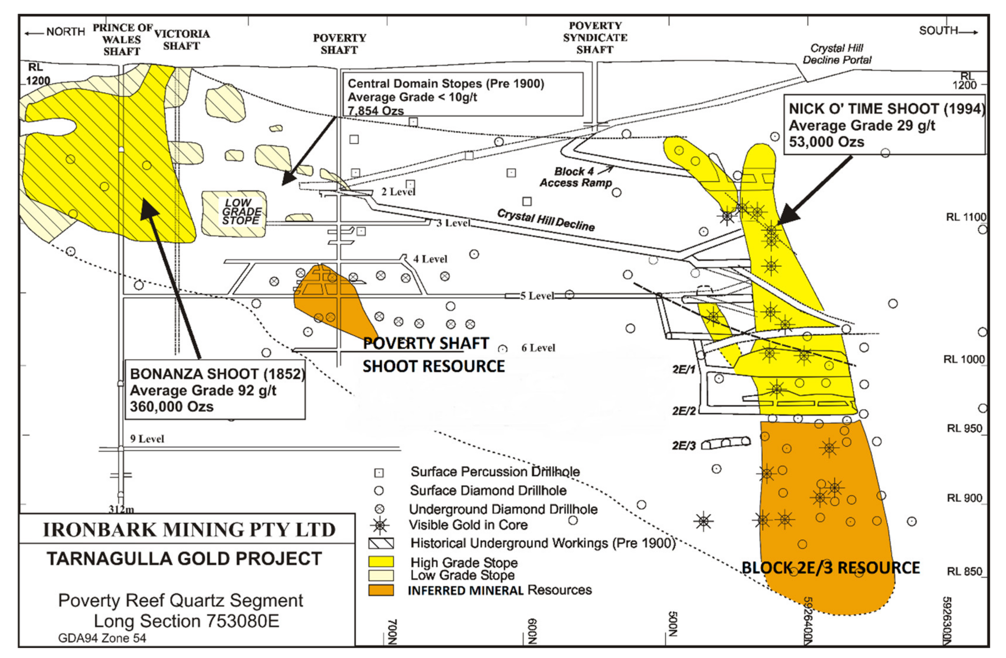
3. Case Study: Crystal Hill Mine, Nick O’Time Shoot

3.1. Introduction

The Crystal Hill mine is located within the Tarnagulla goldfield at the edge of the Tarnagulla township, Central Victoria, Australia. It sits within the world-class Central Victorian Goldfield [46]. Reef Mining NL discovered a high-grade blind shoot, the Nick O’Time shoot (NOT) at the southern end of the Poverty reef in 1994 (Figure 3).
The NOT was mined underground between 1996 and 2000 at Crystal Hill to a depth of 250 m via a decline (Figure 2). It yielded 57,400 t at a head grade of 29.1 g/t Au for 53,000 oz Au recovered [48].
The NOT was discovered in 1994 by surface diamond drilling on a 50 m grid pattern. In 1995, an Inferred Mineral Resource of 30,000 t at 30 g/t was defined for the NOT. On commencement of mining in 1996, the resource was progressively increased based on 15–20 m spaced underground diamond drilling and development. Throughout the project life, the global estimate of grade was reasonably close to that mined but, on a stope-by-stope scale reconciliation was less reliable. No mining has been undertaken in the NOT since 2000. An estimate of the remaining mineralisation is 70,000 t at 5–6 g/t Au (diluted to 2 m) below the 950 m level (Figure 3, Block 2E/3 resource; [47]). It is unlikely that this possesses reasonable prospects for eventual economic extraction at the current time.

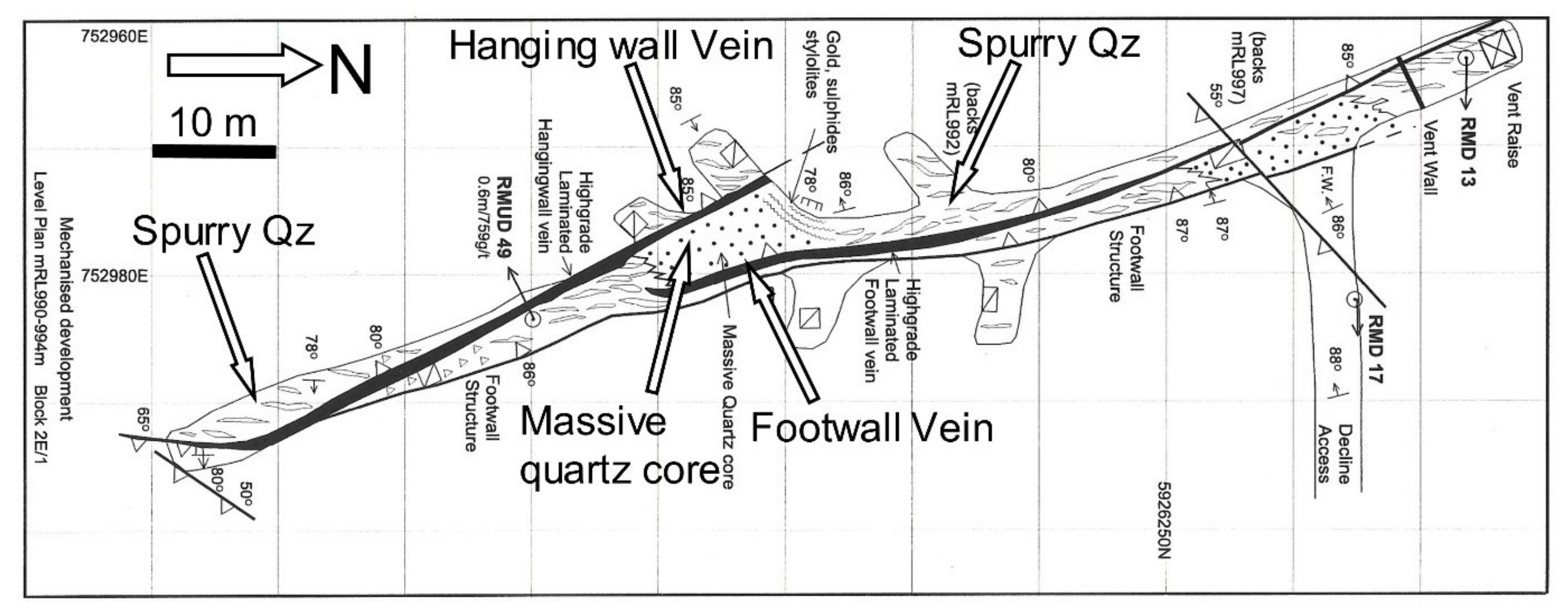
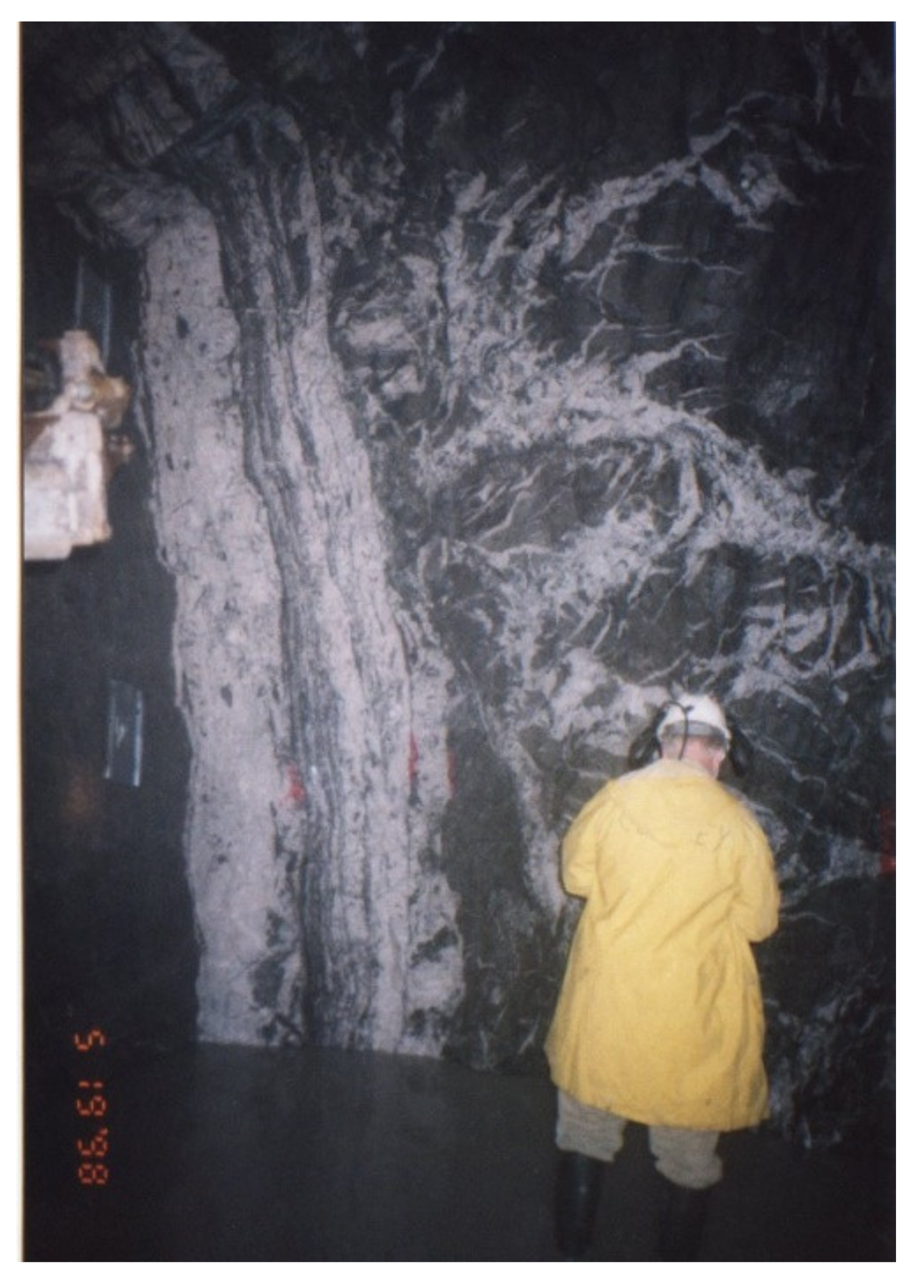
3.2. Geology and Mineralisation

The goldfield is located near the western margin of the Bendigo Zone in the western Lachlan fold belt. The region consists predominantly of deep marine Ordovician turbidites (black shales) which have been metamorphosed to lower greenschist facies and folded into a north-south trending series of chevron folds. Further detail on Tarnagulla regional geology is given in Krokowski de Vickerod et al. [49].
The NOT is located on a steep fault cutting the breached Poverty syncline. The top of the shoot is 70 m below the surface and in longitudinal section is ‘banana-shaped’ and pitches southwards (Figure 3 and Figure 4) [49,50]. The shoot strike length varies from 20 m at the top to 35 m in the middle and to 80 m in the lower section (Figure 3 and Figure 4). The shoot comprises laminated (LV) and spur veins, which vary in width from 0.2 m to 1.8 m and <0.5 m to >3 m, respectively (Figure 5).
In plan, the shoot has a lens shape with a pipe like core of massive low-grade (1–5 g/t Au) white quartz (Figure 4). High-grade gold-sulphide LV, the hangingwall vein and footwall vein, occur along hanging wall and footwall of the pipe (Figure 4 and Figure 5). The hangingwall vein extends south away from the massive quartz core (pipe-like), crossing to the footwall of the gross reef before tapering. This forms a narrow high-grade ‘tail’ to the shoot (Figure 4). The footwall vein extends to the north, moving away from the reef footwall as it tapers.
Table 2 summarises the quartz vein domains identified in the NOT, and the gold type identified in each, and indicates if they were reviewed in this study.
The LV footwall and hangingwall structures host most of the gold mineralisation (>85%). Gold is often associated with sulphide minerals including, pyrite, chalcopyrite, arsenopyrite, sphalerite and galena. The quantity of sulphides associated with gold mineralisation varies vertically in the NOT. Block 4 (at the top of the NOT) exhibits sulphides co-existing in large masses up to 0.3 m wide in the LV and with gold grades up to 2000 g/t Au. The lower blocks (e.g., 2E/1, & 3) in comparison have less sulphides.
During operation, a series of selective mining parcels of spur and/or core zone mineralisation were processed to yield a composite grade of 1.9 g/t Au from 2712 t. This reaffirms the low-grade nature of the spur and core zone mineralisation.

3.3. Statistical and Spatial Characteristics of Gold Grade

The NOT grade control database contains over 600 samples collected from the hanging- and foot-wall LV, and wallrock and spurs veins. LV grades range from 0.04 g/t Au to 3105 g/t Au, with a length-weighted mean of 140 g/t Au. The grades have a coefficient of variation 195% and skewness of 3.8. LV thickness ranges from 5 cm to 1.8 m, with a mean of 0.7 m. Spur vein grades range from 0.02 g/t Au to 20.1 g/t Au, with a length weighted mean of 2.5 g/t Au. The grades have a coefficient of variation of 75%.
Analysis of the combined LV grade data indicates four grade domains (Table 3 and Figure 6), with a major breakpoint at 20 g/t Au.
Above 20 g/t Au (52%), the population contains 98% of contained gold. Underground face mapping indicates that the <20 g/t Au population bears minimal visible gold, whereas the >400 g/t Au population relates to common visible gold. The >2000 g/t Au population relates to abundant visible gold and gold particle clustering, typified by the material described in Section 3.5 and Section 4.
Table 4 shows an analysis of grades based on vertical elevation within the shoot (Figure 3). This shows a reduction in grade with depth, which is also reflected in the resource grade of 6 g/t Au below the 990 m relative level (“RL”).
Two-dimensional variographic analysis was undertaken of the hanging- and foot-wall LVs (Table 5). The global nugget effect is 65%, which indicates a strong degree of grade heterogeneity. The range in the strike direction is relatively short at <9 m and down dip <30 m.

3.4. Ore Characterisation: Thin Section and Hand Specimen Mineralogy and Metallurgical Composite Testwork

3.4.1. Mineralogy

A mineralogical study was undertaken on 126 two by three cm polished thin sections of LV between 1999 and 2003. Most of the polished sections were taken from metallurgical samples MET2 to MET4, which were sourced from the mine during 1999 and 2000 (Table 6).
Several research-level microscopes with graticules for measurement were used in the study. For each gold particle encountered, the long and short dimensions were recorded. Dimensions were reduced to the equivalent circular diameter for comparison.
The 126 sections provided a total study area of c. 756 cm2 based on approximately 45 g of rock slices. Across all sections, 755 gold particles were identified ranging from 15 µm to 4250 µm in size. Approximately 35% of particles were <200 µm in size. The gold generally occurs in quartz in association with pyrite, arsenopyrite, galena, sphalerite, and chalcopyrite. Microprobe analyses of gold revealed fineness values of between 966 and 984, where 102 analyses representing 52 gold particles gave an average fineness of 971.
Figure 7 shows an arsenopyrite-gold assemblage from strongly laminated quartz vein material (from MIN1). The arsenopyrite forms irregular aggregates of subhedral to euhedral crystals. Coarse gold ranges from <15 µm up to 300 µm illustrating the <200 µm range. Most of the smaller particles are enclosed entirely in quartz. The larger particles mostly occur at the margins of the arsenopyrite. They mould against arsenopyrite facets and are partly enclosed in quartz. One large gold grain occurs in a microfracture within arsenopyrite. The textural relationships indicate that gold is later than the coarse arsenopyrite, with some later than the microfractures.
Figure 8 shows some larger coarse gold grains in a gold-galena-pyrite assemblage from the strongly laminated quartz from MIN1 sample. The section was taken from an underground exposure grading 450 g/t Au over 40 cm. The micrograph shows a gold-galena-pyrite assemblage as an aggregate in quartz. Rounded contacts are seen between gold and galena. One gold particle is largely enclosed in quartz and local crystal facets seen on pyrite and quartz.

3.4.2. Metallurgical Testwork

Historical metallurgical testwork and bulk sampling programmes demonstrated that the ore had a substantial gravity recoverable gold (GRG) component. Production processing of 57,400 t resulted in a total gold recovery of 98.5%, with 77% achieved by gravity.
A 50 kg sample (MET1) was tested via the three-stage GRG test at McGill University [51]. The sample assayed at 39 g/t Au, contained 97% GRG, most of it coarser than 100 µm (>85% > 100 µm). At P100 850 µm, 79% of the gold was recovered. The GRG content increased to 90% at an P80 of 170 µm, reaching 97% at an P80 of 75 µm. Some 36% of the recovered gold was <200 µm in size.
For this study, testwork composites were collected from locations underground in 1999 (MET2 and MET3) and in 2000 (MET4 and MET5) (Table 7). Composites were collected from stockpiles, re-muck bays or in situ exposure. In all cases, 20% of the composite comprised LV material, thus approximating 0.7 m of LV with 2.8 m of spurry wallrocks (based on a 3.5 m mining width). MET5 was a spur vein sample.
Samples were processed using the procedure provided in Table 8. Prior to testwork, a 30 kg sample of vein material was used for crush/grind parameter establishment. For each crush/grind step, the product target was between P100 to P90.

3.5. Descriptions of Samples Used for XCT Study

3.5.1. Introduction

Ten samples (D1–D4 and B1–B6) of vein material were acquired from existing collections (Figure 2 and Figure 9). All samples were collected from the upper levels (>1000 m RL: Blocks 2W, 3 and 4) of the NOT and represent high-grade LV material reflected by the presence of visible gold. Nine of the ten samples were scanned by XCT.

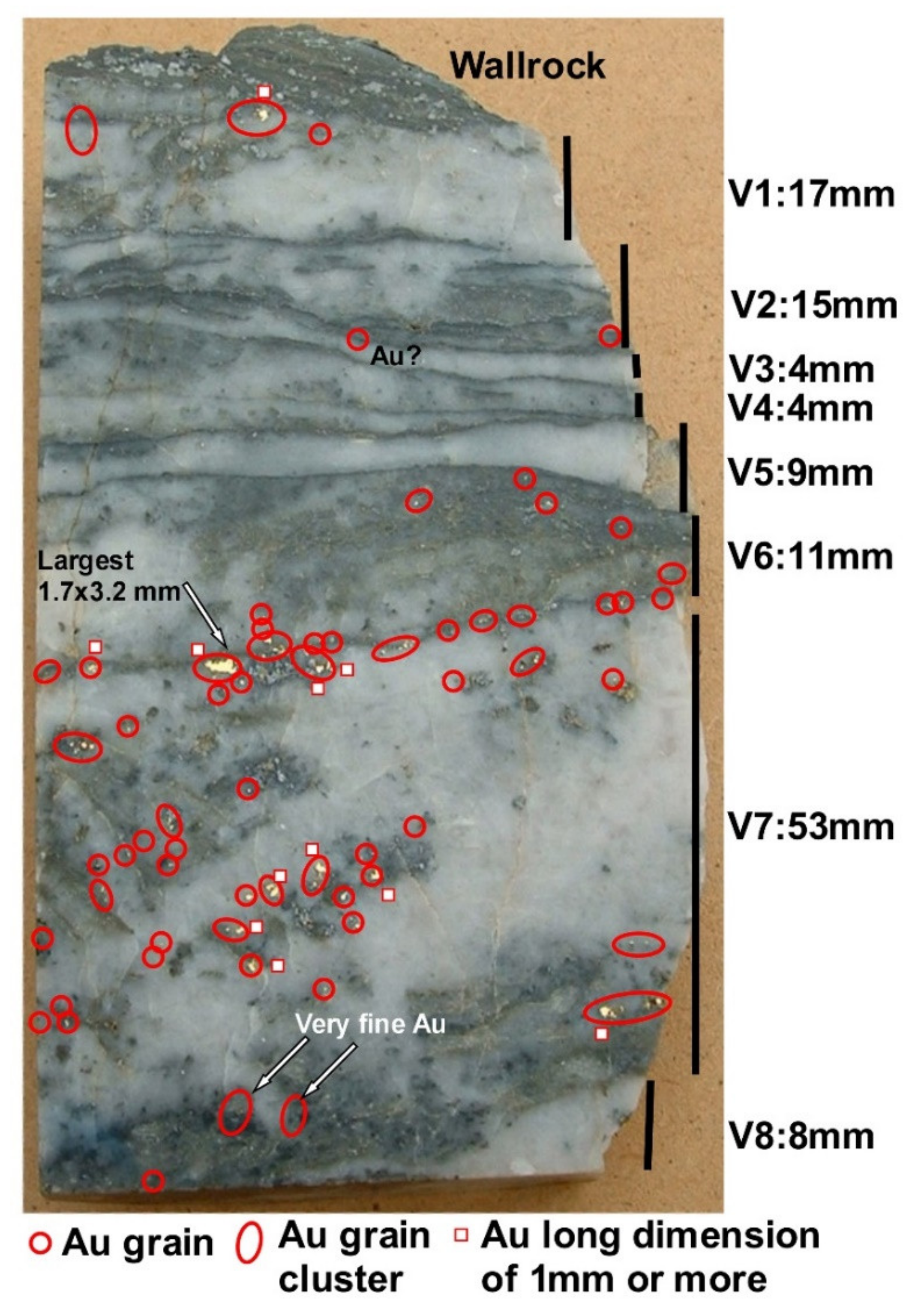
3.5.2. Mineral Fills

Samples show material composed of arrays of 3–8 narrow (<1–8 cm thick) zones which are inferred to represent individual dilational veins (Figure 9). Vein structures in the samples are not significantly damaged by the shear and pressure solution effects reported elsewhere [49].
Vein fills are dominated by quartz, including white and clear varieties. The common sulphides in the XCT set are arsenopyrite and galena with pyrite, marcasite, chalcopyrite and sphalerite also recognised (Figure 9, Figure 10 and Figure 11). In B5 (Figure 9) arsenopyrite is the only sulphide found in V1 (visible in Figure 9), V2, V4, and V6, but V7 is characterised by galena with some arsenopyrite. V3 and V5 lack sulphides and there are local sulphide free domains in V7. Sample B6 conspicuous, coarse altered sulphides and traces of galena adjacent to virtually sulphide free V2 and V3, and D2 shows altered sulphides and galena in V2 adjacent to sulphide free V1 (Figure 10D).
Galena is the most abundant simple sulphide in the XCT set and is commonly associated with gold (Figure 10A,B,D). It is never euhedral, forming irregular equant particles. Aggregates of galena particles are common and usually irregular in form, with quartz indenting the outline. Small aggregates, single particles and sheets and trails of small particles occur in quartz.

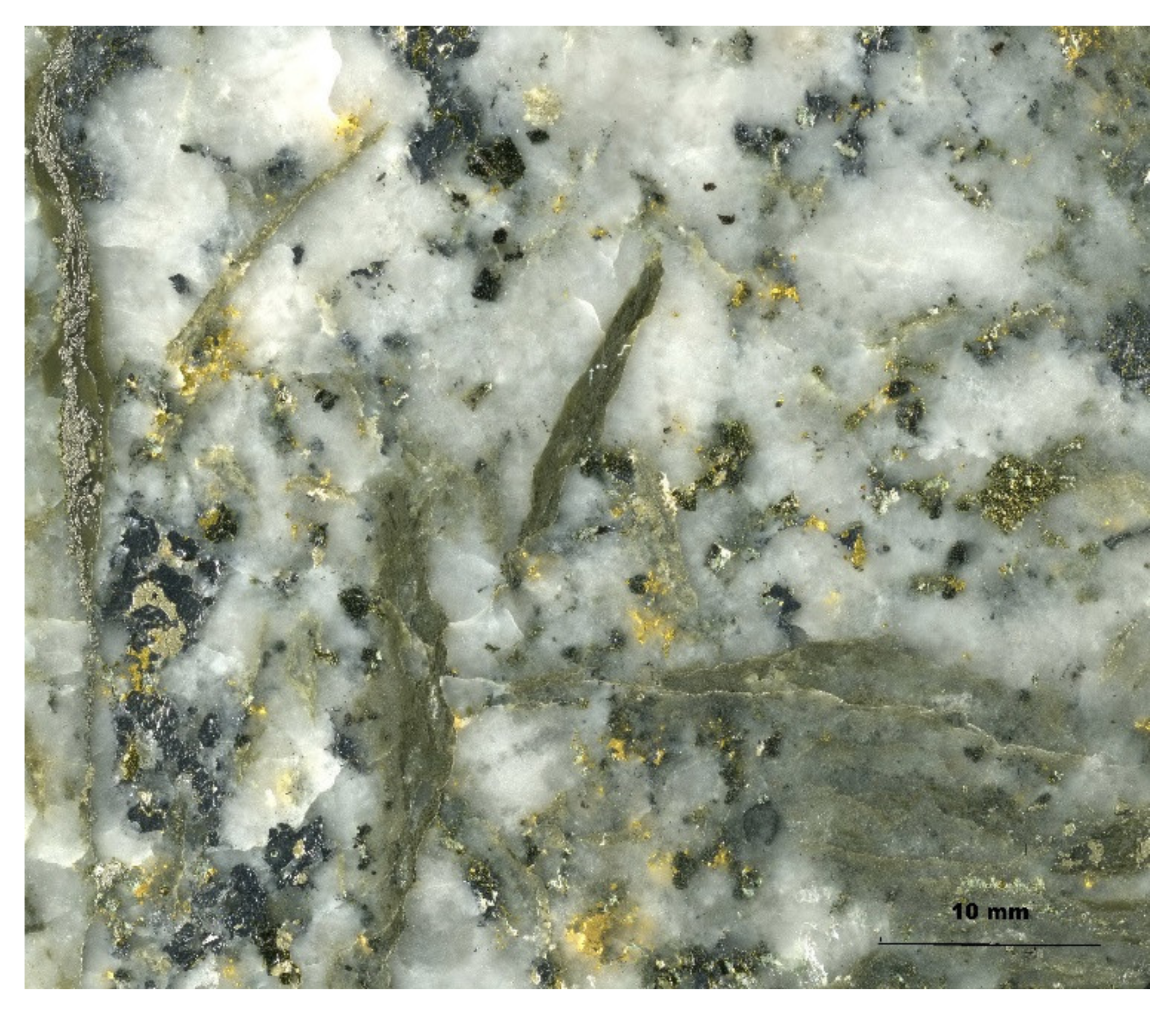
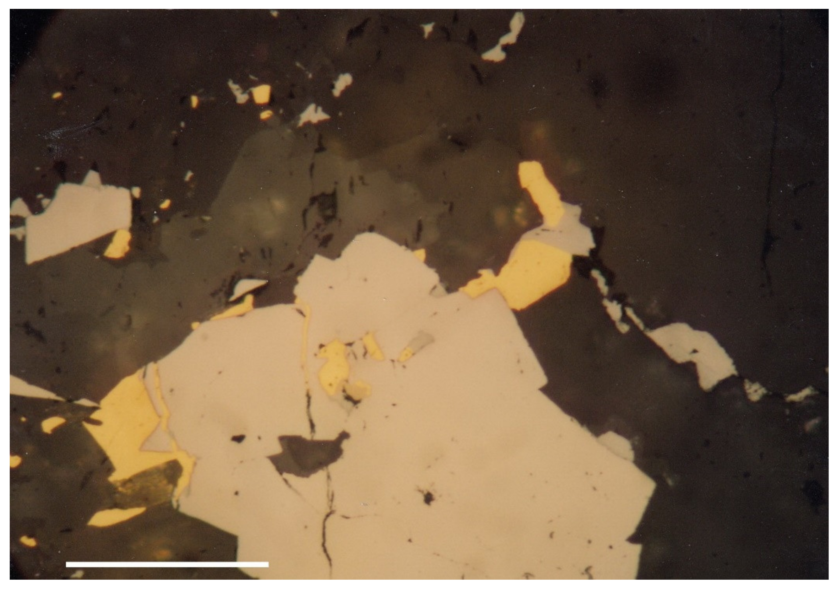
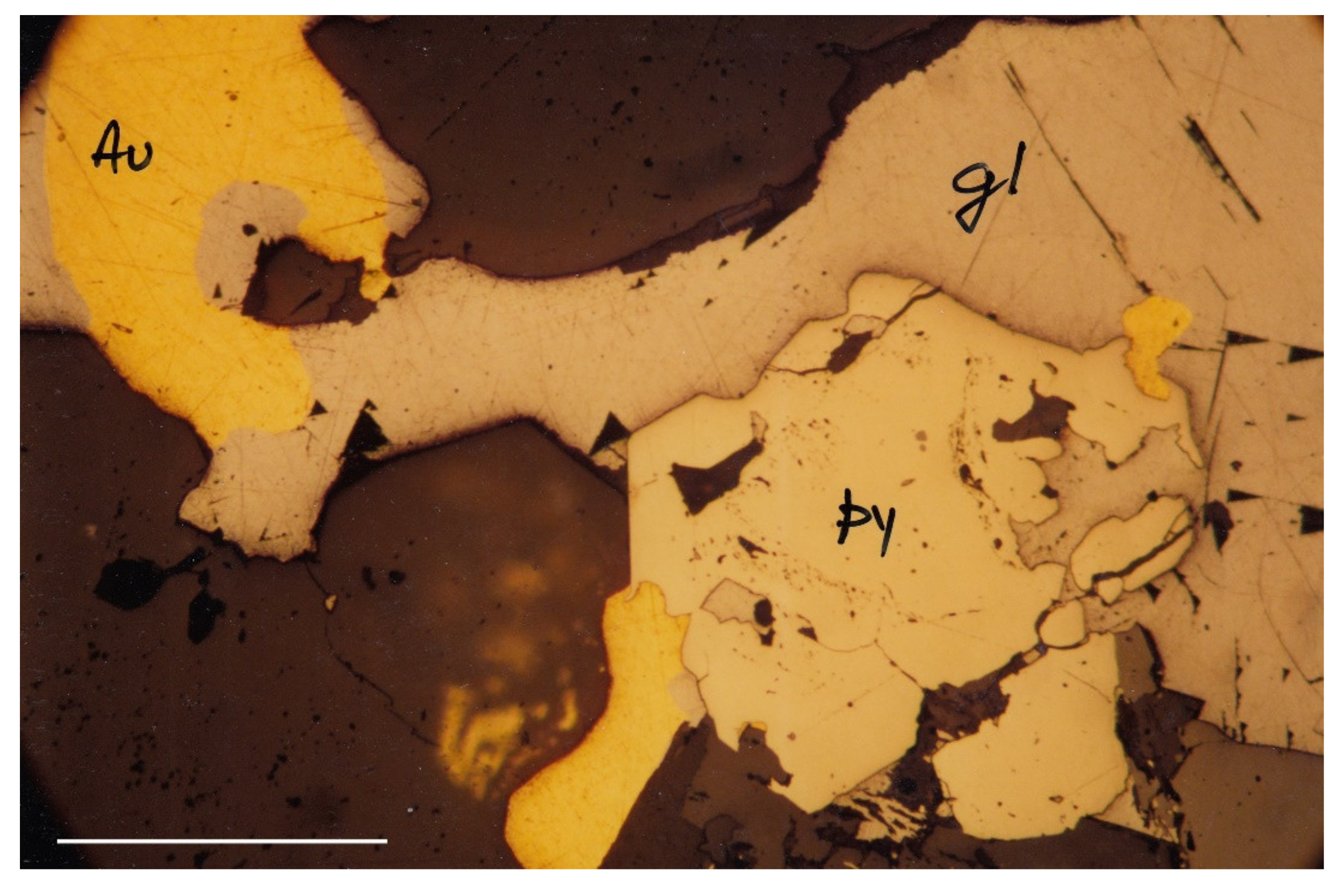
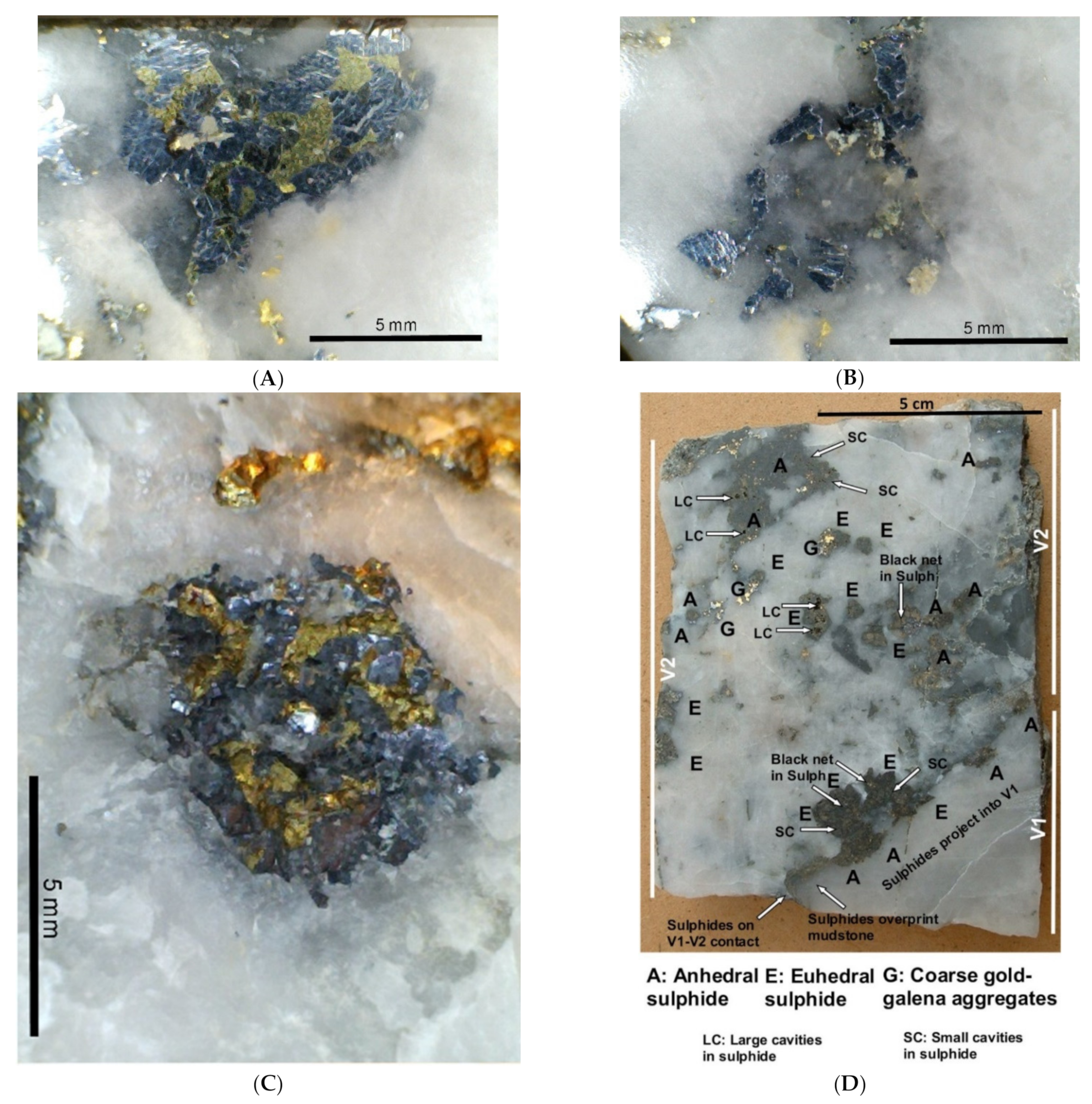
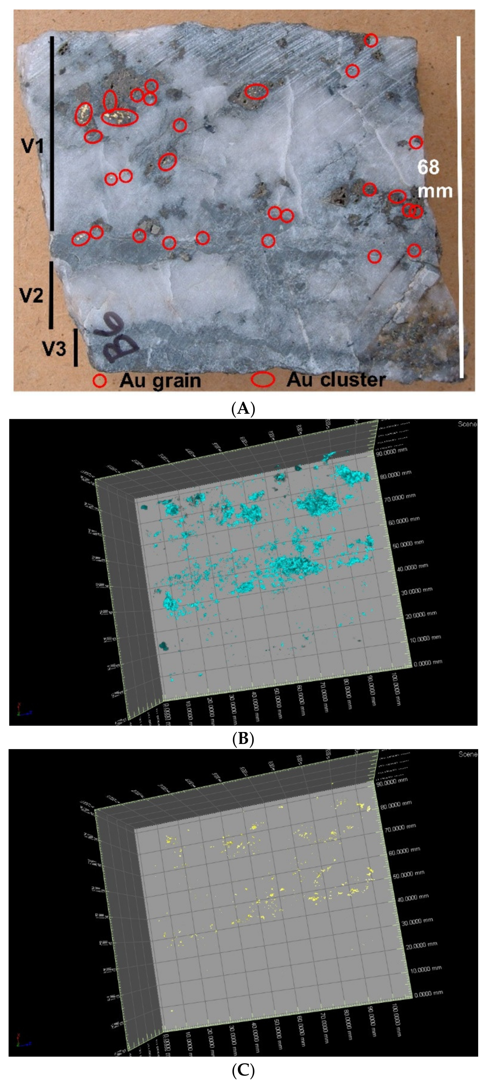
3.5.3. Gold Appearance

Gold particle textures and setting are illustrated in Figure 9, Figure 10 and Figure 11. Gold is irregularly distributed in the samples, producing clusters at different scales and settings. Gold content varies between the component veins in the sample. In B5 (Figure 9) veins V4, V5 and V8 lack gold, minor gold occurs in V1 and V6, whilst gold is abundant in V7. Gold is abundant along some screens (V6 and V7), but rare or absent on others. In B6 gold is common in V1, much of it hosted in altered sulphide (Figure 11E), but only 3 gold particles are seen in V2 and V3.
Gold does not appear to be uniformly distributed in the individual veins. Instead, it forms clusters of various sizes. In sample B5 (Figure 9), vein V7 shows small (<1 cm) clusters of particles, larger (1–3 cm) clusters and these build a vein scale cluster. There is a distinct concentration of gold particles along the mudstone lined contact between V6 and V7 (Figure 9 and Figure 10A). Small clusters are present in most other samples (Figure 10 and Figure 11), with some being in or associated with the altered sulphides and galena aggregates.
Notable is the wide range of gold particle sizes illustrated in Figure 9, Figure 10 and Figure 11. The range is illustrated in V7 of B5. The largest particle seen on any surface was 4.3 mm by 1.9 mm. Particles from 3.2 mm by 1.7 mm to 0.5 mm are seen on Figure 9, particles of 100–500 µm in Figure 11A, and particles from 50–150 µm in Figure 11F, with particles <50 µm identifiable on the sample. Sample D2 shows a comparable range with the coarsest associated with galena, visible in Figure 10D. Examples of the finer gold particles are seen in Figure 11. The ranges are comparable with those identified in the MIN1 and MIN2 studies (Figure 7).
Isolated gold particles set in quartz are moulded against quartz facets (Figure 11C); sheet-like particles and sheets of small particles that follow a net-like pattern possibly marking quartz-quartz grain boundaries (Figure 11B,D); irregular equant particles (Figure 11A, particle 1); rounded particles (Figure 11C); and combinations (Figure 11D). Gold particles are commonly associated with galena (Figure 10A,B,D and Figure 11A). They occur immediately adjacent to galena particles, but not inside individual galena particles. Gold in the galena particle aggregates is found between the component galena particles.

4. XCT Scanning

4.1. Introduction to XCT

High-resolution XCT provides a non-destructive method for analysing mineral particles and textures in rock samples [36,52,53,54]. It can be used to calculate the modal abundance, particle size and distribution of gold in the entire 3D volume of a sample, which other more traditional techniques such as scanning electron microscopy analyses and physical assays cannot (Table 9). The advantage of measuring the 3D characteristics of mineral particles by XCT is that the stereological issues which bias polished sections are removed.
The method uses X-rays to generate a 2D radiograph/shadowgraph of a sample, where differences in greyscale represent changes in X-ray absorption, which is a function of the thickness, density, and atomic number of the materials in a sample. A series of 2D radiographs is acquired over 360° of rotation and the data reconstructed into a stack of virtual slices which can be used to generate a computerised 3D virtual model of the sample.
XCT can rapidly acquire high resolution 3D datasets of gold-bearing samples, typically quarter to one hour per scan depending on size and abundance of gold in the sample. However, accurately processing large numbers of samples to extract quantitative statistics can be difficult and time consuming. Howard et al. [55] discuss the problems with the manual processing of data and look at implementing a protocol and dedicated software to calibrate and normalise XCT data and allow automatic processing.
Minnitt et al. [56] present the first account of using XCT to determine dℓAu based on some South African Witwatersrand gold ores. They note considerable discrepancies between XCT and DSA testwork results. Dominy et al. [36] present a study based on high-grade visible gold ore from the Nalunaq mine, Greenland. They conclude that the XCT outputs are in broad agreement with previous mineralogical and metallurgical studies, though need to be integrated with those studies to resolve gold particle sizing below 150 µm.

4.2. Data Acquisition, Image Processing and Validation

4.2.1. Data Acquisition and Image Processing

The samples B1–B6 and D2–3 was scanned by XCT (Table 10) using a Nikon Metrology (Derby, UK) HMX ST225 XCT system housed at the University of Leicester, Leicester, UK. Machine operating conditions were 225 kV with between 170 µA and 280 µA, using a tungsten target and 4.5 mm copper filter. Some 3142 projections per sample were used.
The voxel dimension of the original scan will determine the effective resolution of the XCT data. In this case, the voxel dimensions are 100 µm thus the effective resolution is 200 µm if it is assumed that at least two voxels are required to define an object [55]. Therefore, any gold particles with a diameter smaller than the effective resolution were not accounted for.
Scanning of geological samples encompasses a greater range of material densities than medical scanning and thus, standards which span a broad range of densities are required [55]. The standards used in this study consist of 2.5 cm discs of polytetrafluoroethylene (2.2 g/cm3), aluminium (2.7 g/cm3), titanium (4.5 g/cm3) and steel (7.85 g/cm3). The calibration uses the actual density of the standards, giving a true density scale once normalised.
The volume of gold was calculated from XCT data after it was segmented in VGstudiomax to distinguish gold from the sample matrix material. The segmentation is achieved by thresholding of the grayscale frequency distribution plot of the dataset. The volume calculation is a mathematical integration calculation of the grayscale frequency distribution curve represented by the segmented phase. By manipulating the greyscale frequency distribution histogram for each dataset, mineral phases were segmented from the bulk rock, allowing their visualisation in 3D. As the composition of a gold particle can be variable within a sample and between samples, depending on the gold-silver compositional ratio, a single threshold value for gold was not applied. However, because gold is the densest phase in the sample and has a density value significantly greater than the next densest phase, sulphide, the lower threshold value that depicts this phase is all that is required and is approximately the same value between samples.
The images have been processed to show the shape of the sample surface, low-density sulphides (e.g., pyrite, marcasite, arsenopyrite and sphalerite), and high-density sulphides (e.g., galena) and gold particles. The different low-density sulphides are not differentiated by XCT. The classes are differentiated by colour in the images, quartz, and wallrock, white; low density sulphides, peach/brown; high density sulphide, blue; and gold, yellow. The results from different density classes can be shown together in an image to identify the relative location of phases. The resulting images, featuring gold particles and aspects of sulphide mineralogy, are then compared with the hand specimen descriptions.

4.2.2. Validation

The nine scanned samples could not be cut, so validation using scanning electron microscopy (SEM) was not extensively undertaken. The polished face from sample D3 was analysed in a LEO 1455 (Thornwood, NY, USA) variable pressure SEM, located at the Natural History Museum London, allowing elemental mapping and backscattered electron imaging of the surface. Energy dispersive X-rays were mapped and recorded using an Oxford Instruments (Abingdon, UK) X-Max silicon drift detector. The 2D elemental maps and backscattered electron image of the sample were analysed using the threshold and measurement tools in ImageJ to determine the area of gold on the sample face. Comparison between the SEM element mapping and XCT images indicated no significant differences.
For all samples, the detailed hand specimen review (Figure 2, Figure 9 and Figure 10D) enabled the XCT scans to be visually checked against surface features. No significant differences were found, and observed gold, sulphides and silicates were effectively represented.
In addition, sample B1 was also scanned by XCT at the Natural History Museum London using the same equipment and operating conditions. Video outputs from both sets of scans were compared visually for gold and sulphide distribution. No significant differences were found.

4.3. Example XCT Results from Samples B5 and B6

4.3.1. Sample B5

The sample is illustrated in hand specimen (Figure 9, Figure 11A,F and Figure 12) and XCT image (Figure 12) with the raw XCT gold particle sizes given in Table 10. Figure 9 provides the hand specimen data with the polished surface in the plane of the page. Figure 12 shows the polished surface viewed obliquely and the top tilted slightly away from the observer.
Figure 12B shows arsenopyrite (brown) as euhedra in the wallrock, the abundant large particles obscure internal details in the image. Arsenopyrite forms conspicuous continuous sheets along the V4/5, V5/6 and V6/7 contacts.
Figure 12C shows galena particles in blue/green with gold in yellow. The general galena distribution matches well with the hand specimen observations: most abundant in V7 but patchy, being absent or rare in the part adjacent to V8 and within parts of the quartz dominated region on the right. The dense blue areas in V7 appear to indicate a dense mass of galena not visible in either Figure 9 or the reverse side of the slab.
Figure 12D shows gold particles with a pattern like that in Figure 9: abundant in V7, much smaller quantities present in order of decreasing amount in V6, V1 and V8. No gold is shown in V2–V5. This generally consistent pattern gives confidence that gold particles are being successfully imaged. Only one surface gold particle from Figure 9 is identified, the 1 mm particle near the wallrock contact of V1.
The gold particles on the far left on the cut side of the slab decrease in abundance towards the sample margin in a manner consistent with the inferred 3D shape of the large gold cluster in V7. The internal structure of the cluster shows smaller sub-clusters differentiated by particle size and spacing. Discrete gold free volumes occur within the cluster, the largest matching with white quartz on Figure 9 and on the reverse of the slab.
The galena-gold association noted in hand specimen is also seen in the images. Comparing Figure 12C,D shows that the general gold distribution is like the galena distribution. The gold particles in V1 all sit on galena particles in Figure 12C. In V6 gold particles are seen both on galena particles and on their own. Some galena particles have no associated gold. Similar relationships are seen in V7 away from the dense galena areas, with gold also adjacent to galena particles.
Gold particle size as shown on Figure 12C,D, ranges from 4 mm longest dimension down to a few hundred microns. The XCT equivalent sphere diameter for B5 is given in Table 10, with a maximum of 2100 µm and mean of 530 µm. The largest gold particle seen in Figure 9 (1.7 mm by 3.4 mm, Figure 10C shows 90–850 µm gold, and Figure 11F shows gold to <50 µm. There is a distinct cluster of >2 mm particles in V7 in the image that shows particles larger than those visible at the surface of the hand specimen (Figure 9).

4.3.2. Sample B6

The sample shows three parallel component veins (V1–3) which are separated by local mudstone screens (Figure 13A). V1 has parallel layers of psuedomorphs after coarse sulphide suggesting crustified vein fill. Galena is present in or adjacent to psuedomorphs, particularly associated with the coarse gold clusters at the top left of Figure 13A. There are no relicts of the pseudomorph pre-cursor, so mineralogy is unknown but most likely to be a sulphide phase.
Gold is common in V1 but rare in V2 (two particles from whole sample) and V3 (one particle from whole sample) (Figure 13A). Figure 11E shows detail of gold clustered in part of a pseudomorph. Figure 11C (particle 1) shows rare, isolated gold in quartz, burying terminations on clear quartz crystals. The XCT scan (Figure 13C) shows abundant gold in V1, most associated with the two layers of pseudomorphed sulphide. There is little gold in the rest of the sample, one particle in each of V2 and V3, both matched with hand specimen. Gold is rare in the large areas of white quartz in V1 occurring in the centre and on far left (Figure 13A,C), effectively holes in the gold distribution in V1.
Gold particle ESDs recorded by XCT are a maximum of 1200 µm and mean of 440 µm. The two largest gold two particles seen in hand specimen are 1500 µm by 600 µm and 1700 µm by 600 µm. The latter almost touches another large particle and the two appear as a single, elongate 3000 µm particle in Figure 13A. These are associated with a pseudomorph which carries galena. The smallest particles are 100 µm, seen in a cluster of 100–500 µm particles in a pseudomorph (Figure 11E).
The gold in V1 occurs in clusters up to 6 mm diameter in V1 (Figure 13A). The whole of V1 in the sample, measuring 40 mm by 80 mm by 24 mm, is characterised by these small clusters. As such, in the context of the whole LV, it potentially represents part of a gold cluster >8 mm3 (Equivalent spherical diameter [ESD] >1.25 mm). This may be an indication of a hierarchy of clusters.

4.4. High Resolution XCT

To investigate potential improved gold particle size resolution, a single 6 mm diameter (240 mm3 volume) plug was drilled out of sample D4. Sample D4 contained trace visible gold, though the plug was purposefully drilled away for this occurrence. This was run using the Australian National University helical cone-beam tomography scanner. The scan resolved gold particles down to 5 µm. Relatively disseminated gold particles up to 50 µm were observed, which displayed a spatial association with undifferentiated sulphide phases. Hand specimen observation of D4 confirms the presence of galena and arsenopyrite.

5. Gold Particle Size Analysis: Integrating Mineralogical, Metallurgical and XCT Testwork

5.1. Limitations of the Testwork Methods Applied in This Study
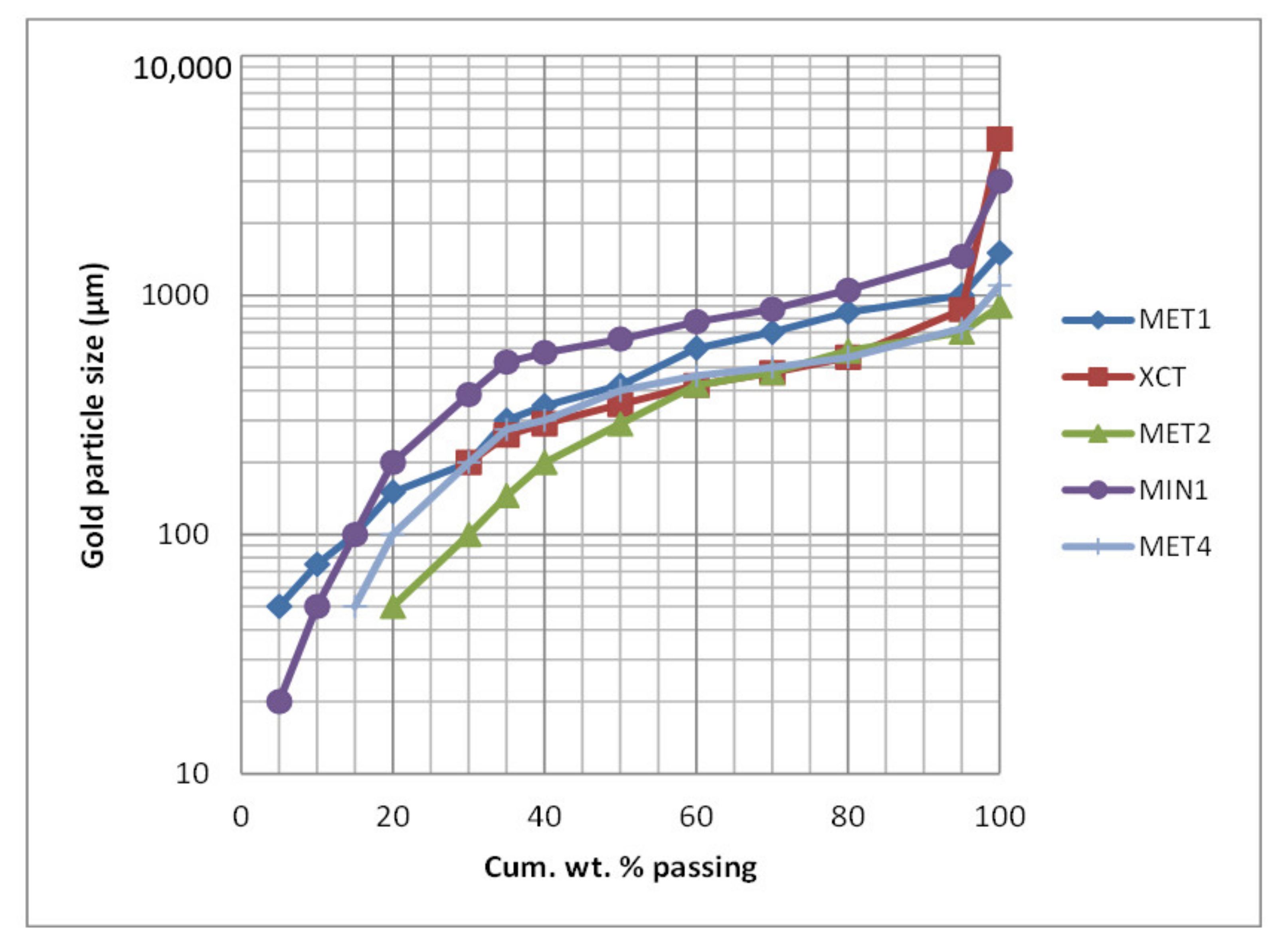
Three characterisation techniques were used during this study: optical mineralogy, metallurgical testwork and XCT; each have limitations (Table 11).
Appropriately sized metallurgical samples are likely to be more representative, though comminution to liberate gold affects the particle size profile. Optical mineralogy is prone to well-known stereological issues. Many polished thin sections are likely to be required to provide a representative count of gold particles, particularly in low grade material. In this case, 126 polished thin sections were studied.
The XCT method provides a method to characterise the in situ nature of mineral particles of contrasting densities. These studies are effective in the study of gold and other very high-density particles. The advantage of determining 3D characteristics by XCT is that the stereological issues which bias polished sections are removed. Continuous XCT scanning of drill core is the goal and would provide many advantages to a project across early stage commencement, automation, and speed (e.g., Orexplore technology).

5.2. XCT Data

All samples analysed by XCT were used for statistical analysis of the gold particle population (Table 12). The ESD was determined from the XCT software particle volume output. Because of software processing issues, the particle size data need to be scaled for analysis and as a result, the effective resolution deteriorates. For this study, all particle size data have been used and the results accord with the hand specimen and optical microscopy studies.
The critical issue is that the particle population is not representative of the total population in each sample due to XCT resolution (i.e., in situ particles below 200 µm in size are not reported). It effectively represents only the coarse fraction of the gold. Based on metallurgical testing (MET1 and MET4), some 30% of gold is less than 200 µm in high-grade ore (>30 g/t Au).
The data from the samples were combined to yield a total population of 6463 particles. The population 95th percentile (P95) was 930 µm. If the population is corrected for the missing 30% of <200 µm particles, the P95 value reduces to 850 µm. Review of a log-probability plot of the raw XCT data indicates a tri-modal population with break points at 400 µm and 1000 µm. The first break point may indicate a change from relatively fine gold/low grade (background) gold, through to a very coarse population related to higher grades above break point two.

5.3. Combined XCT, Metallurgical and Mineralogical Data

5.3.1. Visible-Gold Strongly Laminated Veins

The distribution of gold particle sizes in LVs, determined using XCT and other methods are presented in Figure 14. The metallurgical data were based on both GRG testing (MET1) and sequential grinding, screening, and assaying (MET2 and MET4). Gold was liberated sequentially, which will have resulted in some particle denudation and flattening. The dℓAu value ranges from 1000 µm for MET1, to 700 µm and 725 µm, respectively for MET2 and MET4.
The XCT based curve represents in situ gold particle distribution, corrected for 30% of gold below 200 µm unresolved by XCT. The raw dℓAu value is 930 µm and the corrected value 850 µm. The mineralogical (MIN1) study showed relatively coarser gold, which is likely to be a feature of a 2D analysis and relatively small data population. The MIN data indicate 20% of the gold population is below 200 µm, based on an effective optical resolution of 15 µm.

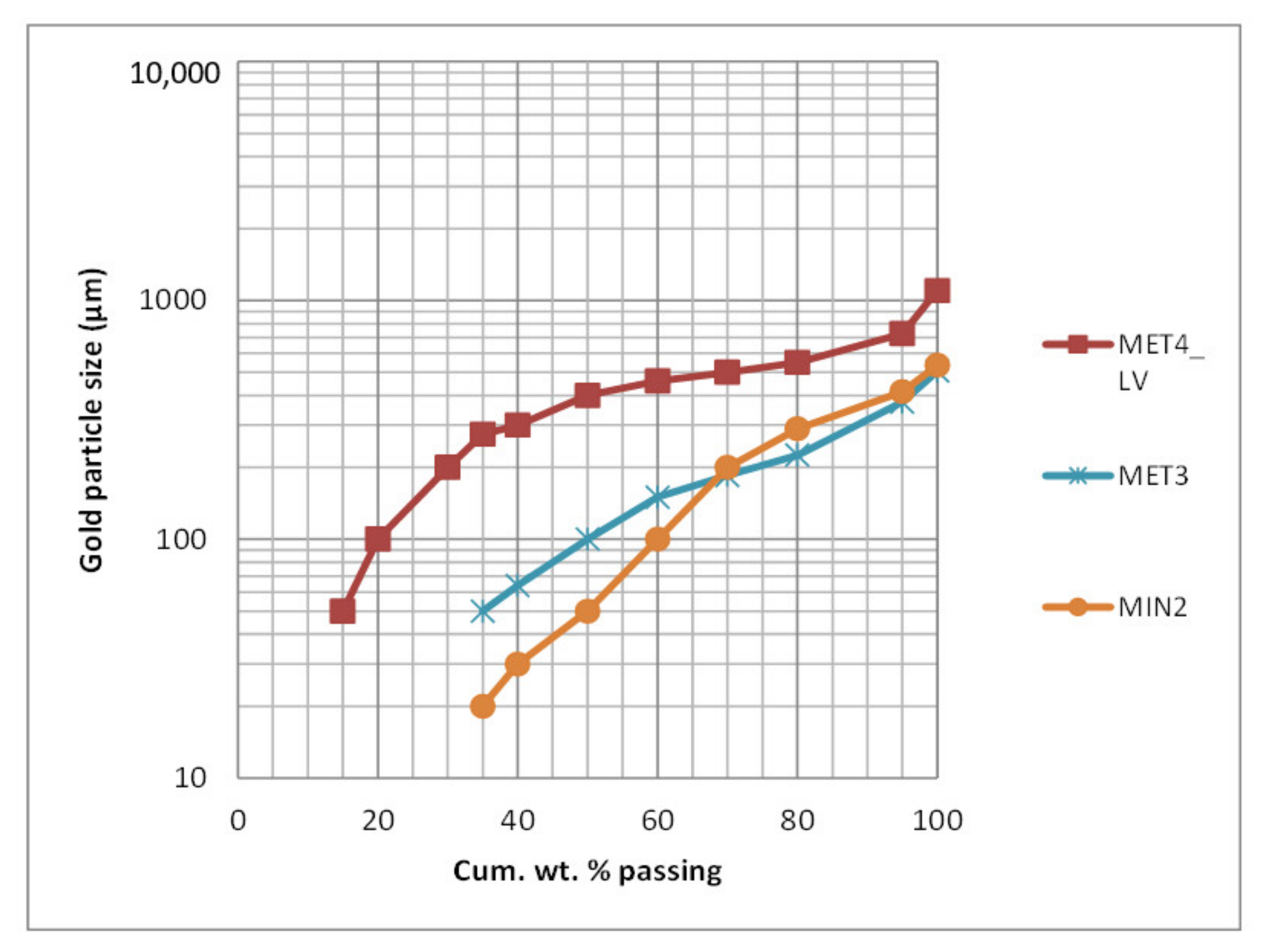
5.3.2. No Visible-Gold Weakly Laminated Vein

The distribution of gold particle sizes from WLV with no visible gold in mineralogical and metallurgical testwork is presented in Figure 15. The metallurgical data were based on sequential grinding, screening, and assaying (MET3). The dℓAu value is 375 µm. The mineralogical (MIN2) study showed relatively coarser gold, which is likely to be a feature of a 2D analysis and relatively small data population. The gold particle distribution of the weakly LVs is notably finer than the strongly LVs, e.g., 50% >100 µm versus 80% >100 µm.

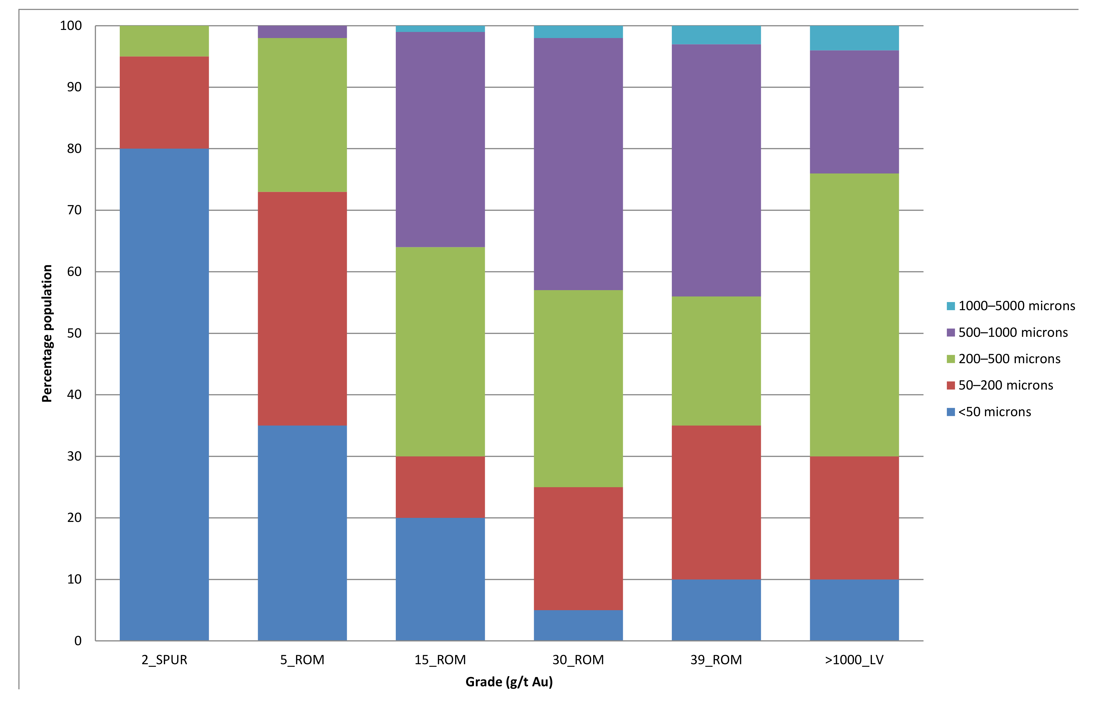
5.4. Gold Distribution by Grade

The NOT ore contains a dominant coarse gold population like other Central Victorian deposits such as Bendigo and Ballarat (e.g., 85% >100 µm and 60% >1000 µm, respectively [9,12]. For NOT ROM ore, 80% of grade relates to >100 µm gold (Table 12; MET4). As grade decreases, the proportion of coarse gold generally reduces. Screen fire assay of core and chip samples confirm more gold in the <100 µm fraction than in grades below 5 g/t Au. This is also confirmed in the MET2 and MET3 samples (Table 12). Gold particle size distributions across low to ultra-high-grade ore are shown in Figure 16.
Test samples MET2, MET3 and MET4 (mean grade 23 g/t Au) show that 30% of the gold is below 200 µm in size. The ultra-high-resolution scan of D4 confirmed the presence of disseminated gold particles between 5 µm and 50 µm in size. The low-grade spur veins (MET5) show extremely low coarse gold content (12% >100 µm) compared to the LV material.

5.5. Gold Distribution by Fraction in ROM Ore

The gold distribution and number of particles by fraction was estimated for ROM ore from the data presented in Figure 16. An effective ESD value was estimated for each fraction using the 70th percentile [37]. The results are presented in Table 13, which shows that 92% of ROM grade is contained in 4% of the estimated contained gold particles. This estimate does not include any consideration of gold particle clustering.

5.6. Calculated Grade of XCT Samples

The XCT gold particle size output can be used to estimate a gold grade for each scanned sample (Table 14). As expected, the XCT identified extremely high grades running into the 1000s g/t Au.
The XCT grade is the grade based on the XCT identified gold only. The estimated head grade includes the estimated 30% fine gold component unresolved by XCT.

5.7. XCT Outcomes

The outcomes of the XCT study are summarised in Table 14 and Table 15. The findings corroborate previous work identifying the coarse nature of the gold and clustering effects. It is important that the gold population characterised by XCT is put into an entire population context. Without the conditioning data of previous mineralogical and metallurgical work, the XCT study was unable to place the coarse gold population into the total (coarse >200 µm and fine <200 µm) gold context.
Visible gold-rich samples such as those from the NOT can be problematic under XCT due to interferences such as star and streak artefacts [53,55]. For many deposits, this type of high-grade ore is not representative of the whole orebody and more likely represents rare high-grade patches. The material studied here is believed to be reasonably representative of the ultra-high grade laminated quartz veins, but not the “average” run of mine ore. The impact on sampling optimisation is discussed in the next section.

6. Sampling Optimisation: In Situ Representative Sample Mass

6.1. Representative Sample Mass: Single Particle Liberation Diameter and Small Cluster (<5 mm) Scenarios

This study uses an approach like that described by Stanley [38] to achieve a precision of ±20% (68% confidence limits). Across the NOT, gold is observed as single particles or as sub-1 cm clusters. A series of dℓAu and dℓclus scenarios were obtained from the mineralogical and metallurgical programmes. RSM values for these scenarios are given in Table 16.
For a ROM ore face at 29 g/t Au, the RSM is 5–6 kg. Once clustering is introduced, the RSM rises to 200 kg (face) and 45 kg (LV). The BCOG is a critical parameter in any operation, and one where sampling protocols are often optimised [59]. In this case, the face RSM for the BCOG is 8 kg, rising to 100 kg if clustering is present. The values across the LV-only are 5 kg and 10 kg.
Gold particle clustering (<5 mm), as observed in hand specimens, polished thin sections and in the field, has a marked effect on the RSM [19,21]. Based on field observation, clustering in lower grade material (<15 g/t Au faces) is considered rare, however at grades approaching the ROM face grade clustering is not uncommon.

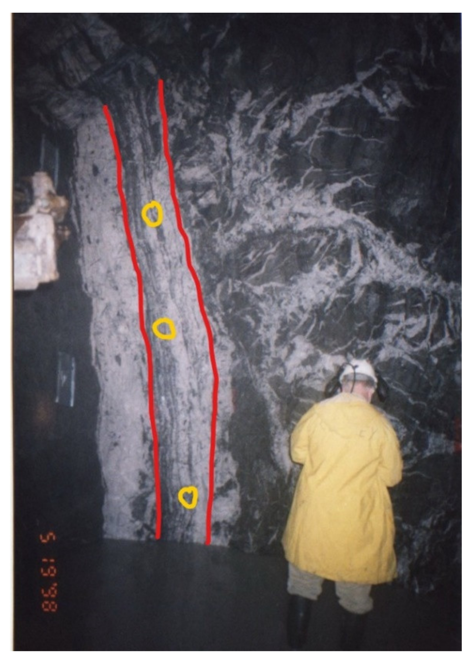
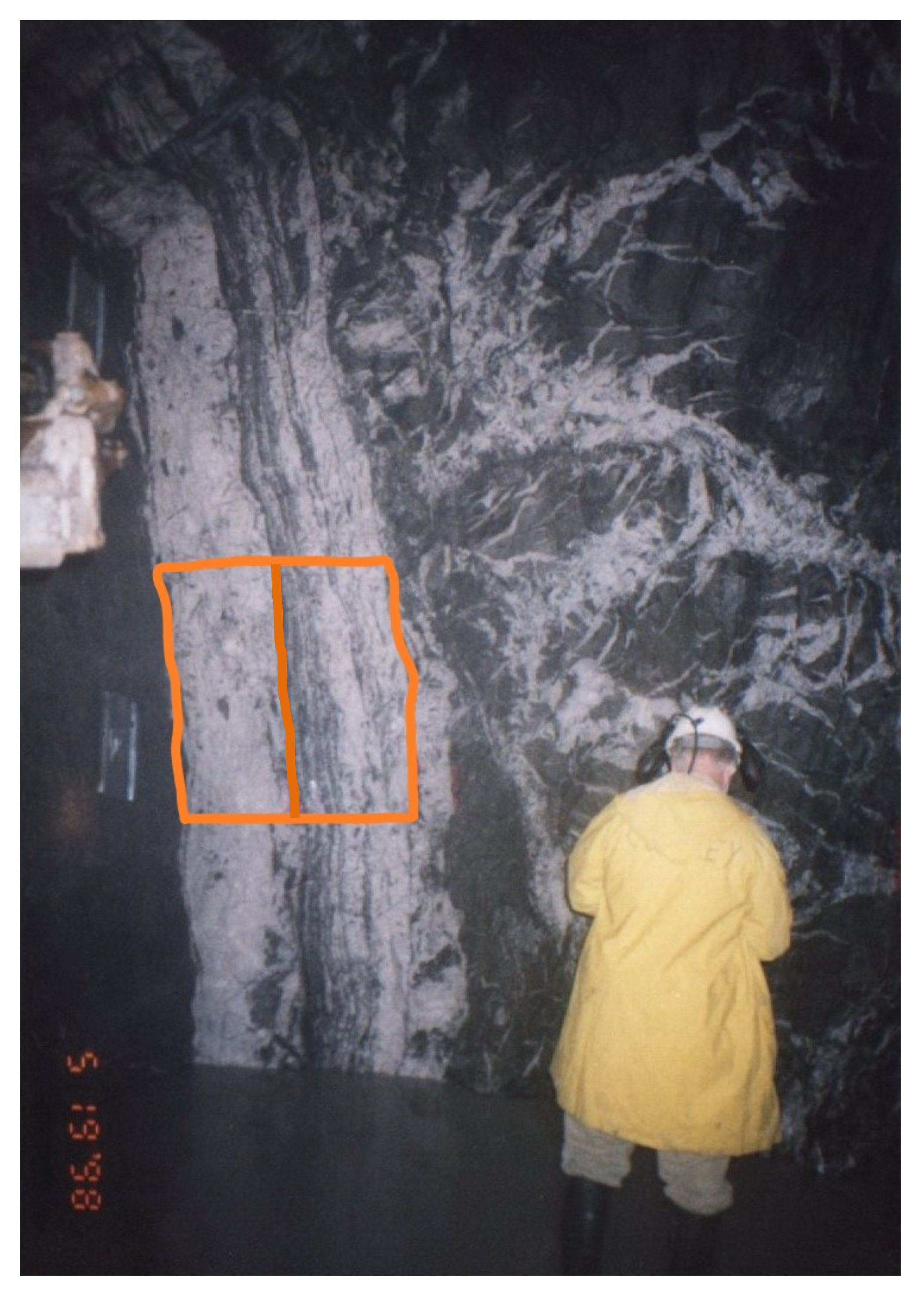
6.2. Representative Sample Mass: Ultra-High Grade Laminated Vein Gold Particle Clustering on Faces

This section investigates face RSM values where ultra-high-grade clusters occur in the upper sections of the mine above 990 m RL. The diluted face grade, assuming an LV grade of 6900 g/t Au (Table 14) is 1200 g/t Au. Although it is based on over 1000 grade control samples taken during production, this figure is clearly too high. The full-face grades range between <0.04 g/t Au and 225 g/t Au with a mean of 26 g/t Au. The grade control programme sampled LV separately to the spur veins and/or barren wallrocks. The LV grade ranged from <0.04 g/t Au to 3105 g/t Au, with a weighted mean of 140 g/t Au. LV widths ranged from 0.1 m to 1.8 m, with an average of 0.7 m. The spur veins generally yielded grades in the range of <0.05 g/t Au to 7 g/t Au, and a mean of 2.5 g/t Au.
From face mapping, the XCT sample determined grade does not reflect the LV material. Whilst visible gold is observed on many faces (generally those >20 g/t Au), it does not dominate, and by area is <20% of the exposed LV. Visible gold may be seen as individual particles up to 5 mm (Figure 11C), as <5 mm scale clusters (e.g., Figure 11A,E,F), and as large <10 cm (e.g., lower part of XCT sample B5; Figure 9) cluster groupings.
Face mapping reveals that ultra-high-grade material occurs locally and may be observed as one to three areas on a face. Rarely did it appear to be more dominant. The 3D continuity of ultra-high-grade mineralisation is unknown, but likely to be relatively short-lived (potentially <1 m along strike). Face separation is 2.7 m in mechanical development, with the difference in LV grade being for example, 1.1 m at 92 g/t Au versus 0.9 m at 1.6 g/t Au in the next face. In another case, two face samples separated vertically by 0.5 m were an order of magnitude different: 953 g/t Au with abundant visible gold versus 29 g/t Au with trace visible gold. The hangingwall and footwall LV are continuous, for example over 65 m along the 965 m level, but the ultra-high-grade occurrences are less so. Figure 17 shows how such ultra-high-grade clusters might occur on an actual face.
Based on field observation, ultra-high-grade zones were unlikely to be more than 100 cm2 patches on the face and potentially not more than 1000 cm3 in 3D. The effect of these 10 cm by 10 cm by 10 cm scale cluster occurrences on the RSM is investigated. Scenario face grades were calculated from different percentages of ultra-high grade LV grading at 6900 g/t Au (Table 9).
RSM values were calculated from the face grade scenarios based on three different cluster sizes (Table 17). The single cluster (one cluster; Table 17) is based on all the gold in the XCT scanned material, agglomerated to give an equivalent spherical gold diameter of 1.2 cm [19]. The other cluster scenarios represent ½ and ⅓ of the single scenario (Table 17).
The results in Table 17 show that when clustering is factored in, the RSM can be substantially higher than when single particle liberation diameter is considered (Table 16). The highest RSM is unsurprisingly for the face BCOG scenario, which reaches 26 t. In this case, face mapping indicates that visible gold of any size is relatively rare in 15 g/t Au or less faces and, when present is observed as single or dispersed particles.
Based on observation, ultra-high-grade material is not expected in faces with a grade of <60 g/t Au, and only as one or two clusters. At higher grades, the RSM values drop below 6 t for all scenarios.

6.3. Representative Sample Mass: Effects of Ultra-High Grade Laminated Vein Gold Particle Clustering

This section investigates LV RSM values where ultra-high-grade clusters occur in the upper sections of the mine (above 990 m RL). Each vein type/domain is likely to possess its own RSM needs based on different grade and dℓAu or dℓclus scenarios [20]. Table 18 shows RSM values for the LV only, applying the >65 g/t Au face scenarios as previously. Given the high LV grades, the RSM values are <1 t and <0.5 t for the grades that are most likely to contain ultra-high-grade mineralisation.
The true proportion of LV containing ultra-high-grade clusters is unknown. An estimate by one of the authors (B.W.C.), suggests overall <10% throughout the NOT. In the upper levels (>990 m RL) this may locally reach around 30% (narrower LVs; 0.1 m to 0.5 m) and in the lower levels (<990 m RL) down to a few percent to zero. In most cases where present, the face grade was >65 g/t Au (>365 g/t Au LV grade assuming a 0.7 m width). In the areas above the 1129 m RL level (Block 4: Figure 3), reconciled head grades were c. 50 g/t Au. Based on field observation, this indicates that the shoot is likely zoned with respect to gold particle clustering and grade, with more ultra-high-grade clusters in the top 60 m of the shoot (Figure 3 and Table 4).

7. Grade Control Sampling, Sample Preparation and Assaying

7.1. Sampling Approach during Production

No DQOs were set for the original sampling programme. Faces were chip-channel sampled across the hangingwall spur veins, LV and footwall spur veins. Chip-channel is a standard underground sampling method, though is not without its weaknesses [59]. The method involves taking a series of chips over a continuous “channel” using a hammer and chisel and/or geopick across the face. Chip-channel sampling is susceptible to high DE and EE errors through operator preference and/or variation in rock hardness [59].
DE reflects poor and variable demarcation of the sample channel. EE is expected to be high, as the sample is chipped out and generally leaves an irregular band in 3D. EE can be extreme if different rock properties are encountered across a sample. The method is prone to operator bias for high-grade sections and/or soft material [59]. For example, where abundant sulphides are present these will break more easily and report to the sample. Where gold is associated with sulphides, this may locally result in a positive grade bias.
At the NOT, chip-channel samples were taken across each face (as a single line) to represent the geological domains present. Samplers were instructed not to bias samples with visible gold and/or sulphides, though reducing this visual bias is hard to achieve in practice. Sample length was restricted to 1 m, with two samples collected if a domain was >1 m. Sample masses were between 5 kg to 10 kg, with a target of 5–7 kg per metre.

7.2. Sample Preparation and Assaying during Production

No DQOs were set for the original sample preparation and assaying programme. All samples were submitted to a commercial laboratory, where they were crushed to P80 −4 mm and riffle split in half. The half was pulverised to P90 −75 µm and split to 1 kg for a 24-h cyanide leach. In some cases, the 1 kg pulp was screen fire assayed. It was not known how the pulps were split, therefore the GSE could have been high and potentially greater than the FSE. Based on the parameters determined here, the FSE was estimated for selected scenarios based on Equation (8) (Table 19).
By domain, the FSE values are generally acceptable (below ±30%), except for the low-grade LV and spur veins. This reflects the low grade of the material and relatively high dℓAu. Where small clusters are present and remain after crushing (e.g., 4 mm crush size versus, for example 2 mm clusters), then the FSE is elevated. Large scale clusters (>1 cm) are unlikely to be an issue, as they would be substantially reduced by the crushing process.
An improvement in the sampling protocol could be achieved by applying a finer crush product. Beyond the FSE several other issues were likely to pervade the sampling protocol. This principally relates to the pulverising of the coarse material to −75 µm. In the presence of coarse gold there is always the risk of gold loss and/or contamination in the pulverising bowl generating PE [8,11,12,22].
The cyanide leach applied for assay is an incomplete gold determination method. Current standard practice is to fire assay the leach tails on a regular basis to monitor leach recovery and reconcile the head grade. This was not done on the NOT samples. Based on limited metallurgical testwork (cyanide leaching for 24 h on P80 −75 µm), at 5 g/t Au recovery is c. 91% and up to 98% for grades >50 g/t Au. Therefore, sample grades are likely to be understated by 2% to 9%.

7.3. Field and Laboratory Duplicate Sample Pairs Analysis

A small number of field and laboratory duplicate pairs are available for LV and spur vein samples. Duplicates allow the analysis of error across the sample collection, sample preparation and assay stages [39]. The target errors for sample collection, sample preparation and assay are <50%, <20% and <10% [59].
The total sampling precision for the LV duplicates is high at ±92%, with the sampling, preparation, and assay component precisions at ±77%, ±51% and ±10%, respectively (Table 20 and Table 21). The laboratory coarse crush duplicate precision is poor at ±50%, which indicates the preparation protocol is not optimal for the coarse gold ore type. The sample collection precision (inclusive of the GNE) swamps the other components, accounting for 69% of all error. As no analytical duplicates were reported, a 10% precision was used. Note the latter was based on analytical duplicates values from another project.
The total sampling error (precision) for the spur duplicates is moderate, at ±38%, with the sampling, preparation, and assays component precisions at ±27%, ±25% and ±10%, respectively (Table 21). The laboratory coarse crush duplicate precision at 25% is relatively high. The sample collection precision dominates the other components taking 50% of all error. No analytical duplicates were reported; therefore a 10% precision was used based on assay duplicate results for the same methodology elsewhere.
In both the LV and spur samples, the sample collection error dominates over the other errors and indicates that the chip-channel process is not optimal. Errors are likely to be driven by samples that are too small, and DE, EE and WE generation during collection. The preparation component errors are also high, indicating sub-optimal sample splitting, crushing and pulverising. Given pulverising of the sample, the effect of liberated gold may have a high impact on the GSE. The analytical error is also high due to the incomplete nature of the assay method.

7.4. Optimisation of the Sample Preparation and Assay Protocol

A key DQO requirement for the preparation and assaying of coarse gold bearing samples, is to avoid gold loss/contamination via liberation (e.g., pulverising) and to achieve total gold assay. In addition, the total sampling error (inclusive of the FSE), excluding the in situ nugget effect, should be less than ±30%.
Two protocols provide an improvement by reducing the FSE and effects of gold liberation during pulverisation (Table 22). Both utilise the non-destructive PhotonAssay method, which is a technology that measures gold concentration via X-ray excitation to produce gamma rays [60]. For grades >3 g/t Au, PhotonAssay provides an analytical precision of ±2.5% or better [60]. PhotonAssay does not solve coarse gold issues per se, however it provides a large charge (e.g., 500 g) or multiple charge (e.g., multiples of 500 g) capability for assaying without the need for pulverisation. The sample needs to be crushed to −2 mm, thus eliminating gold liberation in most cases. The sampling protocol prior to crushing and assaying must be fully optimised.
The reduced FSE values via the two recommended protocols are given in Table 23.
In all but one case, the FSE is reduced below the target 30%. In Protocol 2, the FSE is reduced to zero as the entire crushed sample is assayed. The samples are also not pulverised, so PE gold loss and/or contamination are reduced drastically.

7.5. Actual Sample Mass Compared to RSM

Several RSM scenarios have been presented (Table 16, Table 17 and Table 18). Those deemed likely to be the most material based on knowledge of the NOT mineralisation is summarised in Table 24.
The highest RSM values are observed for the ultra-high grade LV material located in the upper shoot area. Despite the high grade, the large ESD of the clusters drives a high RSM. Without a priori knowledge of ultra-high-grade cluster abundance it is difficult to assess the need for large and impractical sample masses. Smaller samples will most likely understate grade, though collection bias may lead to local overstatement of grade.
During operation, the grade of each development round (the decision unit) was based on the weighted mean of four faces to inform the central round (e.g., four sets of face samples). No geostatistical methodology was applied. Subsequent variography (Table 5) indicates an 8–9 m range in the strike direction, which is nominally four faces (three rounds). The grade was a weighted average estimate made along the entire development drive.
Based on reconciliation with the plant, the weighted average approach using face grades was generally 10–30% higher than that achieved in the plant. This suggests bias in the sample collection process. Avoiding bias due to over-sampling of high-grade areas (e.g., containing visible gold and/or sulphides) and/or softer high-grade material is a common challenge when performing chip-channel sampling [59].

7.6. Recommended Sampling Approach

7.6.1. Protocol

The DQOs for the recommended approach aim to reduce the total sampling errors to less than ±40% compared to the original ±92% (Table 20 and Table 21). The LV sample should be crushed in its entirety to P85 −2 mm and assayed in total via PhotonAssay. Alternatively, the sample can be split in half after crushing, albeit subject to maintaining an acceptable FSE error (Table 25). Combination crusher units (e.g., Rocklabs Boyd smart crusher) can accept a 10–15 kg feed and provide the required 50% split via a rotary splitter.
Given that >85% of the gold is located within the LVs, this should be the focus for more representative sampling. Based on the worst case RSM scenario presented in Table 24 a mass of 45 kg is required. This is however impractical both from a collection and manual handing (transport and sample preparation) perspective. A target LV sample mass of 15 kg per m is recommended, thus providing 11 kg across the mean LV width of 0.7 m. Samples should be collected as panels with a height of 1 m by the vein width (Figure 17). The sample should be collected via multiple continuous chips over the panel area. A well-collected panel sample covers a wider spatial area of the face (Figure 17), based on a large sample collected via contiguous chips taken across the delimited area (Dominy et al. 2018).
The LV varies in width from 0.1 m to 1.6 m, with a mean of 0.7 m. Given this variation, it is suggested that minimum and maximum sample width be set at 0.5 m (7.5 kg) and 1 m (15 kg). A vein <0.5 m should be sampled across 0.5 m including wallrock. An LV >1 m should be sampled as two samples (Figure 18).
In the context of the four-face weighted averaging approach, each round is informed by a total LV sample mass of between 28 kg and 56 kg. This mass range accords with those noted in Table 24 for the LV-only approach. If a kriging approach were used for grade estimation, the search neighbourhood could be informed by between 3 and 12 samples. This provides a total sample mass of between 33 kg and 132 kg, excluding any drillholes that may be present. Proper kriging neighbourhood optimisation would be required.
The spur veins should also be sampled, where a 2 kg per m chip-channel sample should suffice. The spur samples should be collected in 0.5 m ± 0.15 m lengths. Therefore, a 3.5 m wide face with a 0.7 m LV, the spur vein sample should be taken as five 0.55 m samples.
NQ (48 mm diameter at c. 3.5 kg over the mean LV width) diamond core drilling was originally undertaken from surface into the NOT. If continued, whole core or half core assay via PhotonAssay would be recommended to yield an effective FSE of zero.

7.6.2. Sampling Protocol Cost and Value Proposition

The likely cost of the original and recommended protocols is provided (Table 26).
The original protocols are lower cost than the recommended protocols, principally relating to the lower primary sample mass. The single and four sample (four samples to inform the decision unit) total precisions are high. It is estimated that the preparation-assay precision is around ±50%, which is high compared to an acceptable value of <±25%.
The pragmatic solution would be to apply Protocol 1 (Table 22 and Table 26), where half the sample is assayed at a cost of c. A$125 for a single sample precision estimated at <±25%. A duplicate monitoring programme would be required to validate the approach.

8. Conclusions

8.1. General Conclusions

  • Based on the case study presented, mine sampling practitioners can understand the inputs and analysis required to optimise sampling protocols. The approach presented can be applied to fine- or coarse-gold mineralisation to determine the nature of the gold particle sizing and make inferences about the mineralisation.
  • Characterisation of gold mineralisation should be undertaken from the earliest opportunity, whether from diamond drill core or exposure sampling. Integrated programmes of mineralogical and metallurgical testwork provide a direct approach to evaluate the dℓAu and/or dℓclus, and gold particle size distribution. Any such programme has its limitations but will provide better results than more traditional heterogeneity testing.
  • The impact of gold clustering should be evaluated, as it may be significant, influencing the RSM and increasing sample masses to tonnes or even tens of tonnes. Determination of dℓclus is no trivial matter and requires evaluation during surface and/or underground mapping and core logging. While the ultimate resolution of clustering is influenced by XCT, the gold particle size distribution and degree of clustering may vary across the mineralisation.
  • XCT provides an opportunity to study the 3D distribution of gold, and in particular the resolution of clustering. XCT studies must include validation steps and other testwork to resolve gold particle size below the effective resolution.

8.2. Nick O’Time Shoot Conclusions

  • The NOT was domained into low-grade spur vein and high-grade LVs. The LVs can be sub-divided into hangingwall and footwall vein domains, though they are geostatistically, mineralogically and texturally the same so were treated as one. More than 85% of the recovered gold came from the LVs which had a weighted mean grade of 140 g/t Au compared to 2.5 g/t Au for the spur veins. Grade shows a broad zoning, with higher grades in the upper portion of the shoot (>990 m level). Below the 990 m level grade reduces.
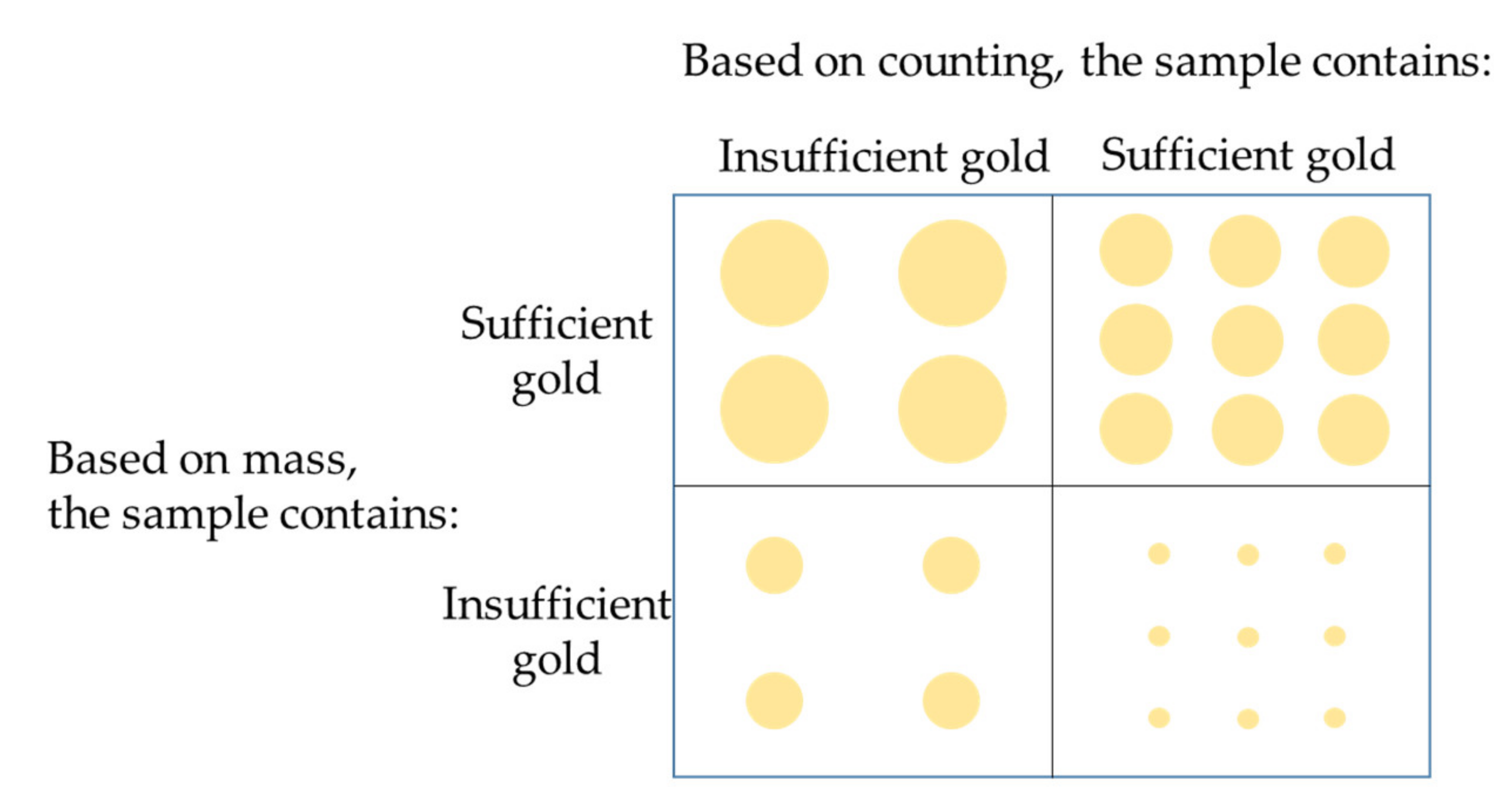
  • NOT is typical of many nuggety deposits dominated by coarse gold where, at a ROM grade of 29 g/t Au, 92% of the contained gold occurs in 4% of the estimated total number of gold particles per tonne. This contrasts with the low-grade spur veins where 80% of the contained gold occurs in 99.8% of the estimated total number of gold particles per tonne. At the mean LV grade of 140 g/t Au, 98% of the contained gold occurs in 12% of the estimated total number of gold particles per tonne.
  • Gold particle clustering on two scales was identified. In ROM and higher-grade mineralisation <5 mm (<65 mm3) scale clustering was observed in thin sections, and mine faces and drill core. At high- to ultra-high grades, >10 mm (>524 mm3) clusters were observed in samples scanned by XCT and field observation.
  • XCT application proved to be effective in defining gold clusters. In addition to the thin section microscopy, it identified a spatial association between gold with arsenopyrite and/or galena. XCT resolved gold particle size to 200 µm, the population below which was defined by reflected light microscopy, metallurgical testwork and high-resolution XCT.
  • LV single particle dℓAu value of 850 µm was recorded for the ROM, with local <5 mm clusters dℓclus values of <3000 µm. At the BCOG, the dℓAu value of 750 µm, with rare dℓclus values of 1500 µm. In high- to very-high grade mineralisation, the same single particle value is appropriate, though >1 cm large cluster dℓclus values range up to 12 cm. Spur veins yield a single particle dℓAu value of 250 µm.
  • A background gold grade population of c. 5–6 g/t Au was identified in the LV domain. This material contains less coarse gold (25% between 200–525 µm) and possesses a dℓAu of 375 µm. Clustering is very rare. The estimated RSM is 5 kg.
  • Given the distinctive grade and textural domains identified at NOT, the approach was taken to optimise RSM by domain (e.g., LV versus spur veins). RSM values for the LV ROM mineralisation are 5 kg for the single particle material, once 3 mm clustering occurs the RSM rises to 45 kg. At very high-grade mineralisation the RSM is 5–10 kg by virtue of the high grade. At the BCOG the RSM is 5–10 kg, and 7 kg for low grade mineralisation. For the ultra-high grade made up of abundant visible gold clusters, RSM values are <1 t and down to 100 kg. The biggest clusters are expected to relate to LV grades of >700 g/t Au for which the RSM is <550 kg.
  • The proposed sampling protocol focusses on the economically gold-bearing LV domain. Larger area panel samples of around 11 kg (over a 0.7 m LV width, approximating to 15 kg per m) are recommended. Two preparation and assay options are suggested based on the PhotonAssay method. In both cases the sample is reduced to P90 −2 mm via a smart crusher, and then either split in half or retained whole. The −2 mm can then be directly assayed via PhotonAssay without the need for pulverising. The 50% sample split option gives reduced FSE values, and the 100% sample option gives a zero FSE. The removal of pulverising from the protocol is particularly valuable, as it reduces the potentially severe effect of the GSE in the presence of liberated gold.

9. Recommendations for the Mine Sampling Practitioner

  • The sampling, sample preparation and assay process should aim to produce a variogram with a <50–60% nugget effect so that estimation variances are as low as possible. To achieve low-nugget variances, larger sample masses must be used when there is a high GNE. They will yield the best estimates of spatial correlation, which in turn will provide optimal SMU grade estimates.
  • Characterisation must start as soon as mineralisation is encountered by outcrop (surface or underground) and/or drilling. At brownfield sites, review of historical information, including core, mapping and metallurgical data can provide data to drive the initial sampling and assaying campaigns. Preliminary dℓAu and/or dℓclus values may be identified and potential worst-case scenarios investigated
  • Initial assaying campaigns should commence with screen fire assaying to identify the presence of coarse gold. This must be backed up by core/exposure logging/mapping to identify visible gold and gold associations. This stage will also identify if clusters are present.
  • When mineralisation is physically accessible or enough core is available, undertake mini-bulk sampling (100–200 kg samples) and testwork, and integrate with mineralogical and metallurgical needs. Testwork should be based on a staged crush-liberation-concentration approach.
  • Sample protocols should be reviewed on a scenario basis and accounting for the correlation of grade with dℓAu (or dℓclus). As a protocol progresses though sample comminution, consideration should be given to the change in dℓAu. Optimisation around the cut-off grade should be investigated as it may be the worst-case scenario.
  • Practitioners should be justifiably critical of face sampling, given its potential for poor precision and high bias. However, it has a role to play in underground grade control, depending on its ultimate use. Maintaining representative samples is advantageous; however, there will always have to be a balance between what is theoretical, practical, and safe. It is important to understand what decisions the sample data will be used for, and the inherent risks involved in that decision process. The removal of face sampling will come from the use of pre-development drilling at a spacing to allow local estimation.
  • Embrace new technologies such as smart crushers and PhotonAssay to achieve large volume assays in a cost-effective way. Any proposed protocol will require validation during initial implementation. This should include review of practical application; collection of duplicates; optimisation of grade control estimates; and reconciliation.
  • There is a need to move towards the quantification of sampling and analytical errors to better communicate uncertainty and risk. A first step is the application of the protocol pro forma and RSV metric presented in Danish Standard DS3077 [61]. Resolution of component relative errors across sampling, preparation and analysis can be gained from the analysis of duplicate sample pairs.

Author Contributions

Conceptualization, S.C.D.; methodology, S.C.D. and H.J.G.; software, S.C.D.; formal analysis, S.C.D., I.M.P., H.J.G. and S.P.; resources, S.C.D.; data curation, S.C.D. and B.W.C.; writing—original draft preparation, S.C.D., I.M.P., H.J.G., S.P. and B.W.C.; writing—review and editing, S.C.D., I.M.P., H.J.G. and S.P.; project administration, S.C.D. and B.W.C. All authors have read and agreed to the published version of the manuscript.

Funding

This research received no external funding.

Data Availability Statement

Not applicable.

Acknowledgments

This contribution is dedicated to co-author Brian W. Cuffley (B.W.C.) who passed away in May 2020. Brian was instrumental in the discovery and mining of the Nick O’Time shoot. Reef Mining NL is acknowledged for access to the Nick O’Time shoot in 1998, 1999 and 2000. XCT scanning was undertaken at the University of Leicester, Natural History Museum London and Australian National University. Reflected light mineralogy was undertaken at Cardiff University, James Cook University and the University of Science and Technology Beijing. Scanning electron microprobe analysis was undertaken at Cardiff University and James Cook University. Metallurgical testwork was undertaken at Cardiff University and the Camborne School of Mines. Tim Evans (formerly Reef Mining NL) is thanked for discussions and provision of data. An early version of this study was presented at the Third AusIMM International Geometallurgy Conference 2016.

Conflicts of Interest

The authors declare no conflict of interest.

Abbreviations

AEAnalytical error
BCOGBreakeven cut-off grade
CLConfidence limits
DEDelimitation error
d or dℓAuLiberation diameter
dℓclusClustered liberation diameter
DSADuplicate series analysis
DQOData quality objective
ESDEquivalent spherical diameter
EEExtraction error
FSEFundamental sampling error
GNEGeological (or in situ) nugget effect
GRGGravity recoverable gold
GSEGrouping and segregation error
HGHigh grade
HTHeterogeneity test
KSampling constant
LVLaminated vein
MLVModerately laminated vein
NOTNick O’Time shoot
PEPreparation error
RLRelative level above a given reference horizon
ROMRun of mine grade
RSMRepresentative sample mass
RSVRelative sampling variability
SLVStrongly laminated vein
SMUSelective mining (or decision) unit
SNESampling nugget effect
TOSTheory of Sampling
WEWeighting error
WLVWeakly laminated vein
XCTX-ray computed tomography

References

  1. Carrasco, P.C.; Carrasco, P.; Jara, E. The economic impact of incorrect sampling and analysis practices in the copper mining industry. Chemom. Intell. Lab. Syst. 2004, 74, 209–214. [Google Scholar] [CrossRef]
  2. Gy, P.M. Sampling of Particulate Materials: Theory and Practice; Elsevier: Amsterdam, The Netherlands, 1982; p. 431. [Google Scholar]
  3. Minnitt, R.C.A. Sampling: The impact on costs and decision making. J. S. Afr. Inst. Min. Metall. 2007, 107, 451–462. [Google Scholar]
  4. Dominy, S.C. Importance of good sampling practice throughout the gold mine value chain. Mining Tech. 2016, 125, 129–141. [Google Scholar] [CrossRef]
  5. Lyman, G.J.; Bourgeois, F.S. Sampling, corporate governance and risk analysis. In We Are Metallurgists Not Magicians: Landmark Papers by Practicing Metallurgists; The Australasian Institute of Mining and Metallurgy: Melbourne, VIC, Australia, 2017; pp. 349–354. [Google Scholar]
  6. Dominy, S.C.; O’Connor, L.; Purevgerel, S. Importance of representative metallurgical sampling and testwork programmes to reduce project risk—A gold case study. Mining Tech. 2019, 128, 230–245. [Google Scholar] [CrossRef]
  7. Pitard, F.F. Theory of Sampling and Sampling Practice; CRC Press: Boca Raton, FL, USA, 2019; p. 694. [Google Scholar]
  8. Royle, A.G. Splitting gold assay pulps containing coarse gold. J. Leeds Univ. Min. Assoc. 1989, 89, 63–68. [Google Scholar]
  9. Johansen, G.F.; Dominy, S.C. Development of Sampling Protocols at the Bendigo Gold Project, Australia. In Proceedings of the World Conference on Sampling and Blending, Sunshine Coast, QLD, Australia, 10–12 May 2005; Australasian Institute of Mining and Metallurgy: Melbourne, VIC, Australia, 2005; pp. 175–183. [Google Scholar]
  10. Cintra, E.C.; Scabora, J.A.; Viegas, E.P.; Barata, R.; Maia, G.F. Coarse Gold Sampling at Sao Francisco Mine, Brazil. In Proceedings of the World Conference on Sampling and Blending, Porto Alegre, Brazil, 23–25 October 2007; Fundacao Luiz Englert: Porto Alegre, Brazil, 2007; pp. 187–197. [Google Scholar]
  11. Dominy, S.C. Predicting the unpredictable–evaluating high-nugget effect gold deposits. In Mineral Resource and Ore Reserve Estimation Guide to Good Practice; Australasian Institute of Mining and Metallurgy: Melbourne, VIC, Australia, 2014; pp. 659–678. [Google Scholar]
  12. Dominy, S.C. Sampling Coarse Gold-Bearing Mineralisation–Developing Effective Protocols and a Case Study from the Ballarat Mine, Australia. In Proceedings of the World Conference on Sampling and Blending, Perth, WA, Australia, 9–1 May 2017; Australasian Institute of Mining and Metallurgy: Melbourne, VIC, Australia, 2017; pp. 71–84. [Google Scholar]
  13. Gonzalez, P.; Cossio, S. A Review of Sampling Protocol for a Gold Ore Based on Liberation Study. In Proceedings of the World Conference on Sampling and Blending, Porto Alegre, Brazil, 23–25 October 2007; Fundacao Luiz Englert: Porto Alegre, Brazil, 2007; pp. 163–174. [Google Scholar]
  14. Pitard, F.F. The Advantages and Pitfalls of Conventional Heterogeneity Tests and a Suggested Alternative. In Proceedings of the World Conference on Sampling and Blending, Bordeaux, France, 10–12 June 2015; IM Publications LLP: Chichester, UK, 2015; pp. 13–18. [Google Scholar]
  15. Villanova, F.L.S.P.; Heberle, A.; Chieregati, A.C. Heterogeneity Tests and Core Logging—A Final Reconciliation. In Proceedings of the World Conference on Sampling and Blending, Perth, WA, Australia, 9–11 May 2017; Australasian Institute of Mining and Metallurgy: Melbourne, VIC, Australia, 2017; pp. 107–113. [Google Scholar]
  16. Dominy, S.C.; Platten, I.M.; Xie, Y.; Minnitt, R.C.A. Underground grade control protocol design: Case study from the Liphichi gold project, Larecaja, Bolivia. Appl. Earth Sci. 2011, 119, 205–219. [Google Scholar] [CrossRef]
  17. Dominy, S.C.; O’Connor, L.; Glass, H.J.; Purevgerel, S. Xie, Y. Towards representative metallurgical sampling and recovery testwork programmes. Minerals 2018, 8, 193. [Google Scholar] [CrossRef] [Green Version]
  18. Arkenbout, A.; Brochot, S.; Esbensen, K.H.; Minkkinen, P.; Holmes, R.J.; Huachang, L.; Dominy, S.C.; Mingwei, Z.; Romanach, R.J.; Robben, C.; et al. Economic arguments for representative sampling. Spectrosc. Eur. 2021, 33. in press. [Google Scholar]
  19. Dominy, S.C.; Platten, I.M. Clustering of gold particles and implications for sampling. Appl. Earth Sci. 2007, 116, 130–142. [Google Scholar] [CrossRef]
  20. Dominy, S.C.; Xie, Y.; Platten, I.M. Gold Particle Characteristics in Narrow Vein Deposits: Implications for Evaluation and Metallurgy. In Proceedings of the Narrow Vein Mining Conference, Ballarat, VIC, Australia, 14–15 October 2008; Australasian Institute of Mining and Metallurgy: Melbourne, VIC, Australia, 2008; pp. 91–104. [Google Scholar]
  21. Pitard, F.F. The In-situ Nugget Effect: A Major Component of the Random Term of a Variogram. In Proceedings of the World Conference on Sampling and Blending, Porto Alegre, Brazil, 23–25 October 2007; Fundacao Luiz Englert: Porto Alegre, Brazil, 2007; pp. 91–110. [Google Scholar]
  22. Dominy, S.C.; Petersen, J.S. Sampling Coarse Gold-Bearing Mineralisation-Developing Effective Protocols and a Case Study from the Nalunaq Mine, Southern Greenland. In Proceedings of the World Conference on Sampling and Blending, Sunshine Coast, QLD, Australia, 10–12 May 2005; Australasian Institute of Mining and Metallurgy: Melbourne, VIC, Australia, 2005; pp. 151–165. [Google Scholar]
  23. Dominy, S.C.; Purevgerel, S.; Esbensen, K.H. Quality and sampling error quantification for gold mineral resource estimation. Spectroscopy Europe 2020, 32, 21–27. [Google Scholar]
  24. Lyman, G.J. and Esbensen, K.H. Critique of Gy’s Sampling Theory–Misplaced expectations of Wikipedia’s democratic intentions. TOS Forum 2013, 1, 28–30. [Google Scholar]
  25. Esbensen, K.H. Introduction to the Theory and Practice of Sampling; IM Publications: Chichester, UK, 2020; p. 328. [Google Scholar]
  26. François-Bongarçon, D.M. Theory of sampling and geostatistics: An intimate link. Chemom. Intell. Lab. Syst. 2004, 74, 143–148. [Google Scholar] [CrossRef]
  27. Pitard, F.F.; François-Bongarçon, D.M. Demystifying the Fundamental Sampling Error and the Grouping and Segregation Error for Practitioners. In Proceedings of the World Conference on Sampling and Blending, Santiago, Chile, 25–28 October 2011; GECAMIN: Santiago, Chile, 2011; pp. 39–56. [Google Scholar]
  28. François-Bongarçon, D.M.; Gy, P.M. The most common error in applying Gy’s formula in the theory of mineral sampling and the history of the Liberation factor. J. S. Afr. Inst. Min. Metall. 2002, 102, 475–479. [Google Scholar]
  29. François-Bongarçon, D.M. Extensions to the demonstration of Gy’s formula. Explor. Min. Geol. 1998, 7, 149–154. [Google Scholar]
  30. Minnitt, R.C.A.; Rice, P.; Spangenberg, C. Experimental calibration of sampling parameters K and alpha for Gy’s formula by the sampling tree method. J. S. Afr. Inst. Min. Metall. 2007, 107, 513–518. [Google Scholar]
  31. Minnitt, R.C.A.; Assibey-Bonsu, W. A Comparison between the Duplicate Series Method and the Heterogeneity Test as Methods for Calculating Gy’s Sampling Constants, K and Alpha. In Proceedings of the World Conference on Sampling and Blending, Cape Town, South Africa, 21–23 October 2009; Southern African Institute of Mining and Metallurgy: Johannesburg, South Africa, 2009; pp. 137–154. [Google Scholar]
  32. Pitard, F.F. Practical and theoretical difficulties when sampling gold. In Proceedings Mineral Processing Plant Design, Practice and Control; SME: Littleton, CO, USA, 2002; pp. 77–89. [Google Scholar]
  33. Bazin, C.; Hodouin, D.; Mermillod-Blondin, R. Reproducibility of Low-Grade Ore Batches Prepared for Metallurgical Testing. In Proceedings of the World Conference on Sampling and Blending, Santiago, Chile, 10–12 July 2013; Gecamin: Santiago, Chile, 2013; pp. 419–433. [Google Scholar]
  34. Dominy, S.C.; Xie, Y. Optimising sampling protocols via the heterogeneity test: Challenges in coarse gold mineralisation. Mining Tech. 2016, 125, 103–113. [Google Scholar] [CrossRef]
  35. Minnitt, R.C.A.; Francois-Bongarçon, D.M.; Pitard, F.F. Segregation Free Analysis for Calibrating the Constants K and Alpha for Use in Gy’s Formula. In Proceedings of the World Conference on Sampling and Blending, Santiago, Chile, 25–28 October 2011; GECAMIN: Santiago, Chile, 2011; pp. 133–150. [Google Scholar]
  36. Dominy, S.C.; Platten, I.M.; Howard, L.E.; Xie, Y.; Bell, R.F.; Minnitt, R.C.A. Determination of the Sampling Liberation Diameter in a High-Grade Coarse Gold Ore by High-Resolution X-Ray Computed Tomography. In Proceedings of the Sampling Conference, Perth, WA, Australia, 21–22 August 2012; Australasian Institute of Mining and Metallurgy: Melbourne, VIC, Australia, 2012; pp. 161–169. [Google Scholar]
  37. Clifton, H.E.; Hunter, R.E.; Swanson, F.J.; Phillips, R.L. Sample Size and Meaningful Gold Analysis, Professional Paper 625-C; United States Geological Survey: Washington, DC, USA, 1969; p. 19.
  38. Stanley, C.R. Nugget calculation parameters for samples and elements affected by the nugget effect. Explor. Min. Geol. 1998, 7, 139–147. [Google Scholar]
  39. Stanley, C.R.; Smee, B.W. Strategies for reducing sampling errors in exploration and resource definition drilling programmes for gold deposits. Geochem. Explor. Env. Anal. 2007, 7, 1–12. [Google Scholar] [CrossRef]
  40. François-Bongarçon, D.M. Fishy Samples: How Big a Sample to Avoid the Infamous Poisson Effect. In Proceedings of the World Conference on Sampling and Blending, Cape Town, South Africa, 21–23 October 2009; Southern African Institute of Mining and Metallurgy: Johannesburg, South Africa, 2009; pp. 43–46. [Google Scholar]
  41. Villanova, F.L.S.P.; Chieregati, A.C. The use of equant grain particles to validate analytical sample size in gold deposits—A case study. Chemo. Intell. Lab. Syst. 2018, 181, 36–44. [Google Scholar] [CrossRef]
  42. Dominy, S.C.; Platten, I.M.; Xie, Y. Determining Gold Particle Size in Gravity Ores for Sampling and Metallurgical Characterisation–Discussion and Test Protocol. In Proceedings of the Gravity Gold Conference, Ballarat, Australia, 21–22 September 2010; Australasian Institute of Mining and Metallurgy: Melbourne, VIC, Australia, 2010; pp. 83–95. [Google Scholar]
  43. Mariano, R.A.; Evans, C.L. Error analysis in ore particle composition distribution measurements. Mins. Eng. 2015, 82, 36–44. [Google Scholar] [CrossRef]
  44. Pitard, F.F. Guidelines for Acceptable Allotted Sampling Uncertainty. In Proceedings of the World Conference on Sampling and Blending, Santiago, Chile, 10–12 July 2013; Gecamin: Santiago, Chile, 2013; pp. 89–98. [Google Scholar]
  45. Graindorge, J. Maintaining Sample Data Quality through Robust Quality Assurance and Quality Control Protocols. In Proceedings of the Sampling Conference, Perth, Australia, 11–12 May 2010; Australasian Institute of Mining and Metallurgy: Melbourne, VIC, Australia, 2010; pp. 111–116. [Google Scholar]
  46. Wilson, J.L.; Moore, D.H.; Vollgger, S.A.; Madeley, H.E. Structural evolution of the orogenic gold deposits in central Victoria, Australia. Ore Geol. Rev. 2020, 120, 103390. [Google Scholar] [CrossRef]
  47. B.W. Tarnagulla Mineralisation Report Including a Grade and Tonnage Estimate for the Nick O’Time Shoot; Unpublished Report for Castlemaine Goldfields Ltd.: Ballarat, VIC, Australia, 2013; p. 45. [Google Scholar]
  48. McCarthy, P.L.; Faulkner, L. Tarnagulla Gold Mine. In Proceedings of the Narrow Vein Mining Conference, Ballarat, VIC, Australia, 14–15 October 2008; Australasian Institute of Mining and Metallurgy: Melbourne, VIC, Australia, 2008; pp. 237–248. [Google Scholar]
  49. Krokowski de Vickerod, J.; Cuffley, B.W.; Evans, T. Tarnagulla Goldfield, Central Victoria. In Victorian Initiative for Minerals and Petroleum Report No 71; Minerals and Petroleum Victoria: Melbourne, VIC, Australia, 2001; p. 160. Available online: http://earthresources.efirst.com.au/product.asp?pID=542&cID=8 (accessed on 28 September 2021).
  50. Cuffley, B.W.; Krokowski de Vickerod, J.; Evans, T.; Fraser, R. A new structural model for fault-hosted gold mineralisation: An example from the Nick O’Time ore shoot, Poverty Reef, Tarnagulla. In Developments in Victorian Geology and Mineralisation; Australasian Institute of Geoscientists Bulletin No. 24: Perth, WA, Australia, 1998; pp. 53–63. [Google Scholar]
  51. Laplante, A.R. Report on the Characterization of Gravity Recoverable Gold in a Sample of Reef Mining NL Ore. In Unpublished Report by the Department of Mining and Metallurgical Engineering; McGill University: Montreal, QC, Canada, 1998; p. 15. [Google Scholar]
  52. Chisambi, J.; von der Heyden, B.; Tshibalanganda, M.; Le Roux, S. Gold exploration in two and three dimensions: Improved and correlative insights from microscopy and X-ray computed tomography. Minerals 2020, 10, 476. [Google Scholar] [CrossRef]
  53. Kyle, J.R.; Ketcham, R.A. Application of high-resolution X-ray computed tomography to mineral deposit origin, evaluation and processing. Ore Geol. Rev. 2015, 65, 821–839. [Google Scholar] [CrossRef]
  54. Guntoro, P.I.; Ghorbani, Y.; Butcher, A.R.; Kuva, J.; Rosenkranz, R. Textural quantification and classification of drill cores for geometallurgy: Moving toward 3D with X-ray microcomputed tomography. Nat. Res. Res. 2020, 29, 3547–3565. [Google Scholar] [CrossRef]
  55. Howard, L.E.; Elangovan, P.; Abel, R.L.; Dominy, S.C.; Armstrong, R. Characterisation of Gold Ores by X-Ray Micro-Computer Tomography Part 1: Software for Calibration and Quantification of Mineralogical Phases. In Proceedings of the International Geometallurgy Conference, Brisbane, Australia, 5–7 September 2011; Australasian Institute of Mining and Metallurgy: Melbourne, VIC, Australia, 2011; pp. 321–330. [Google Scholar]
  56. Minnitt, R.C.A.; Collins, D.; Whitten, W.; Gay, S.L.; Louwrens, E.; Morrison, R. Comparison of the Liberation Size Determined by Different Methods. In Proceedings of the World Conference on Sampling and Blending, Porto Alegre, Brazil, 23–27 October 2007; Fundacao Luiz Engler: Porto Alegre, Brazil, 2007; pp. 253–267. [Google Scholar]
  57. Dominy, S.C.; Murphy, B.; Gray, A.H. Characterisation of Gravity Amenable Gold Ores–Sample Representativity and Determination Methods. In Proceedings of the International Geometallurgy Conference, Brisbane, QLD, Australia, 5–7 September 2011; Australasian Institute of Mining and Metallurgy: Melbourne, VIC, Australia, 2011; pp. 281–292. [Google Scholar]
  58. Dominy, S.C.; O’Connor, L.; Glass, H.J.; Xie, Y. Geometallurgical study of a gravity recoverable gold orebody. Minerals 2018, 8, 186. [Google Scholar] [CrossRef] [Green Version]
  59. Dominy, S.C.; Glass, H.J.; Lam, C.K.; O’Connor, L.; Purevgerel, S.; Minnitt, R.C.A. Integrating the Theory of Sampling into underground grade control strategies. Minerals 2018, 8, 232. [Google Scholar] [CrossRef] [Green Version]
  60. Tremblay, C.D.; Tickner, J.; Treasure, D.; Oteri, A.; Wheeler, G. PhotonAssay–Efficient and Bulk Gold Analysis in the Modern World. In Proceedings of the International Mining Geology Conference, Perth, WA, Australia, 25–26 November 2019; Australasian Institute of Mining and Metallurgy: Melbourne, VIC, Australia, 2019; pp. 88–98. [Google Scholar]
  61. DS3077. Representative Sampling–Horizontal Standard; Danish Standards Foundation: Copenhagen, Denmark, 2013; p. 41. [Google Scholar]
Figure 1. High-grade (c. 2700 g/t Au) LV material from the Crystal Hill mine, Australia. Photograph of sample B1 showing individual coarse gold particles between 500 µm to 1500 µm in size.
Minerals 11 01109 g001
Figure 2. Comparison of sample analysis evaluation based on the mass (proportional number of coarse particles) and total number of particles (counting).
Minerals 11 01109 g002
Figure 3. Bonanza and Nick O’Time shoots on the Poverty reef (after [47]).
Minerals 11 01109 g003
Figure 4. Geological plan of the 992 m level, Block 2E/1 in the NOT showing the laminated hanging- and foot-wall veins (black) and central-barren massive-quartz core. Grade of development 20 g/t Au over 60 m strike length (after [47]).
Minerals 11 01109 g004
Figure 5. Hangingwall vein in the NOT at the south end of the 992 m level in Block 2E/1, where three distinct geological domains are observed. The high-grade strongly LV in the centre (0.7 m at 157 g/t Au) is associated with a massive weakly LV (0.5 m at 2 g/t Au). The spur vein zone (2.8 m at 0.5 g/t Au) on its hangingwall. The grade of the LV is 92 g/t Au over 1.2 m. The face grade is 28 g/t Au over 4 m. Brian W. Cuffley for scale.
Minerals 11 01109 g005
Figure 6. Log-probability plot for LV grades based on 625 face samples.
Minerals 11 01109 g006
Figure 7. Strongly laminated quartz vein material from MIN1 comprising individual grains of arsenopyrite and coarse gold. Field of view: 0.7 mm; Scale bar 0.175 mm.
Minerals 11 01109 g007
Figure 8. Strongly LV material from MIN1 comprising coarse gold grains associated with galena (gl) and pyrite (py). Field of view: 1.5 mm; Scale bar: 0.375 mm.
Minerals 11 01109 g008
Figure 9. Sample B5 illustrating features of vein assemblage, mudstone-arsenopyrite screens and distribution of visible gold in laminated reef. V1 shows arsenopyrite-gold assemblage associated with mudstone flakes. V2–V5 shows very narrow veins with minor arsenopyrite with only gold near V2/3 boundary. V7 shows a major gold pocket. Estimated sample grade 4200 g/t Au from XCT.
Minerals 11 01109 g009
Figure 10. Aspects of sulphide occurrence. (A) Sample B1, irregular aggregate of galena particles with other sulphides intergrown. Gold (100–500 µm) present in field of view. (B) Sample B1, chains of single galena particles in clear quartz. (C) Sample B4, galena, chalcopyrite, and clear quartz aggregate filling pseudomorph of euhedral sulphide phase. (D) Sample D2, hand specimen showing altered sulphide with euhedral and anhedral forms, gold is visible in these on the actual sample. The coarsest gold is visible in galena-gold aggregates.
Minerals 11 01109 g010
Figure 11. Aspects of gold occurrence. (A) Sample B5, gold occurrence at the V6/7 boundary in Figure 9. 1, Gold with frilled margin in quartz; 2, possible euhedral particles in quartz; 3, scalloped gold grain on V6/7 boundary; 4, gold particles in galena aggregate; 5, string of small particles along V6/7 boundary; 6 string of gold particles along possible quartz-quartz grain boundary. (B) Sample D2, gold particles and sheets inferred to follow quartz grain boundaries. (C) Sample B6, gold isolated in quartz. 1, gold moulded on quartz terminations; 2 gold with rounded form. (D) Sample D2, small (2 mm) gold cluster. (E) Sample B6, gold cluster (3 mm) in part of sulphide pseudomorph. Gold particles range from 100–500 µm. (F) Sample B5, cluster of small gold particles in quartz with mudstone debris. Core of cluster 2 mm. Particles range from <50–150 µm.
Minerals 11 01109 g011
Figure 12. Images derived from XCT scans of sample B5. Images show a slightly oblique view of the face illustrated in Figure 9 and shows the cut side of the sample slab that is not visible in Figure 9. The background grid is part of the sample co-ordinate system, grid spacing is 10 mm. (A) Sample surface showing position relative to grid and locating veins (V) and wallrock (WR). (B) Full volume of lower density sulphides (arsenopyrite—brown). (C) Full volume of high-density sulphide (galena—blue) with gold (yellow). (D) Full volume of gold (yellow) with sample outline shown by spots.
Minerals 11 01109 g012
Figure 13. Sample B6, photograph and XCT images. The XCT images are viewed in same direction as the hand specimen photograph but are slightly rotated left hand down relative to hand specimen photograph. (A) Hand specimen photograph. Single gold particles (>500 µm) circled in red, gold particle clusters in red ovals. Most gold occurs in, or adjacent, sulphide psuedomorphs. (B) Distribution of sulphides through the sample. (C) Distribution of gold through the sample.
Minerals 11 01109 g013
Figure 14. Gold particle size curves for high-grade LV material. Results plotted: MET1; MET2; MET4; MIN1 and XCT.
Minerals 11 01109 g014
Figure 15. Gold particle size curves no visible gold weakly LV mineralisation (MET3 and MIN2). LV MET4 (ROM grade) data included for comparison.
Minerals 11 01109 g015
Figure 16. Gold particle size distribution across low (2_SPUR MET5: 2 g/t Au; 5_ROM MET3: 5 g/t Au), moderate (15_ROM MET2: 15 g/t Au), ROM (30_ROM MET4: 30 g/t Au) to high (39_ROM MET1: 39 g/t Au) grades, and ultra-high grade (XCT: >1000_LV g/t Au).
Minerals 11 01109 g016
Figure 17. LV (highlighted in red) with spurry veins on its hanging wall. Three theoretical occurrences of potential ultra-high grade are marked for illustration. Occurrences are not necessarily circular. Compare spacing with chip-channel sample collected during mining which was based on a single line across the face.
Minerals 11 01109 g017
Figure 18. Panel sample outlined area on LV (highlighted in orange). In this case, the composite LV is 1.2 m wide and should be collected as 0.5 m (massive LV) and 0.7 m (strong LV) wide panels.
Minerals 11 01109 g018
Table 1. Definition of TOS sampling errors.
Sampling
Error
AcronymError TypeEffect on SamplingSource of ErrorError Definition
FundamentalFSECorrect Sampling Error (CSE)Random Errors-
Precision Generator
Characteristics of the
mineralisation. Relates to
Constitution and Distribution Heterogeneity
Grade heterogeneity of the broken lot. FSE does not cancel out and remains even after a sampling operation is perfect. Experience shows that the total nugget effect can be artificially high because sample weights are not optimal.
Grouping and SegregationGSEError due to the combination of grouping and segregation of rock fragments in the lot. Once rock is broken, there will be segregation of particles at any scale.
DelimitationDEIncorrect Sampling Error (ISE)Systematic Errors-
Bias Generator
Sampling equipment and
materials handling
Incorrect shape of the volume delimiting a sample.
ExtractionEEIncorrect extraction of a sample. Extraction is only correct when all fragments within the delimited volume are taken into the sample.
WeightingWECollection of samples that are of a comparable support. Samples should represent a consistent mass per unit.
PreparationPEIssues during sample transport and storage (e.g., mix-up, damage), preparation (contamination and/or losses), and intentional (sabotage) and unintentional (careless actions and non-adherence of protocols) human error.
AnalyticalAEAnalyticalAnalytical processErrors during the assay and analytical process, including issues related to rock matrix effects, human error, and analytical machine maintenance and calibration.
Table 2. Overview of quartz vein domains and the gold type identified in each.
Quartz Vein DomainStructural Event (1)Domain Grade
(g/t Au)
Visible GoldDisseminated Single
Particle Gold
<5 mm Gold Clusters<10 cm Gold ClustersReviewed in This Work
Core zoneD3A<5
(mean 2 g/t Au)
NoRareNoNoNo
LVD3B140
(weighted mean)
CommonCommonCommonYesMIN; MET; XCT (2)
Spur veinsD3A<5
(mean 2 g/t Au)
RareRareRareNoMET
(1) After [49,50]. (2) MIN: mineralogical study; MET: metallurgical testwork; XCT: X-ray computed tomography.
Table 3. Analysis of the combined LV grade data.
Cumulative Probability RangeGrade Range
(g/t Au)
Mean Grade
(g/t Au)
Contained Gold
P0–480.03–2062%
P48–9120–40010331%
P91–99400–200062637%
P99–100>2000344030%
Table 4. Analysis of grades based on vertical elevation.
Level Interval
(m RL)
BlockWeighted Mean LV Grade
(g/t Au)
Mean LV Thickness
(m)
1129–115543000.35
1050–112931500.75
1032–10502W1250.65
990–10322E/11600.65
965–9902E/2550.55
940–9652E/360.50
Table 5. Variogram parameters.
Laminated Vein DomainNugget EffectStrike RangeDip Range
Hangingwall65%8 m25 m
Footwall65%9 m30 m
Table 6. Summary of mineralogical datasets used in this study.
Data SetLocationDomainSource MET Samples
(Refer Table 7)
No of
Sections
Est. LV Grade
(g/t Au)
MIN1Blocks 2E/1, 2W and 3SLVMET470 >200
MIN2Block 2E/2WLVMET2 and MET35640–60
SLV: strongly laminated vein with abundant visible gold; WLV: weakly laminated vein with minor visible gold.
Table 7. Overview of MET samples collected and tested as part of this study. SLV: strongly laminated vein with abundant visible gold; MLV: moderately laminated vein with minor visible gold; WLV: weakly laminated vein with minor visible gold.
Sample IDMine Block LocationTestwork LaboratoryDomainSample Mass (kg)Sample Grade (g/t Au)Grade Type
MET1Upper (>990 m RL)McGillSLV5039.0High
MET22E/2CardiffMLV25014.9Moderate/BCOG
MET32E/2CardiffWLV2505.2Low
MET42E/1, 2W and 3CamborneSLV25030.4High/ROM
MET5VariousCamborneSPUR2002.1Low
Table 8. Overview of the metallurgical testwork protocol enacted for MET samples 2 to 5.
StageCrush/Grind StepGold ConcentrationGold Particle Size Evaluation
1Crush entire sample to −5 mmScreen product at 2 mm
Pan + 2 mm product
Pass −2 mm fraction over a
Wilfley table
Review each gold concentrate(s) by optical microscopy
Screen gold concentrate at 5000; 1000; 500; 200; 50 µm
Weigh and assay each fraction to extinction
2Crush S1 fraction to −2 mmPass entire fraction
over a Wilfley table
3Crush S2 fraction to −1 mm
4Grind S3 fraction to −0.5 mm
5Grind S4 fraction to −0.2 mm
6Grind S5 fraction to −50 µmBy assayCyanide leach entire fraction; fire assay tails
Table 9. Key outputs from XCT that support sampling optimisation and metallurgical evaluation.
Gold Particle ParameterSampling OptimisationMetallurgical Processing
SizeSize range and dℓAuSize range
ShapeShape and range of shape typesShape and range of shape types
Distribution (incl. clustering)Presence of and degree of clustering (dℓclus)--
Associations--Associated mineral distribution and degree of encapsulation
Table 10. Summary of raw (uncorrected for <200 µm content) gold particle equivalent spherical diameter (ESD) statistics from XCT image analysis.
SampleNumber of Gold Particles IdentifiedMean ESD (µm)Maximum ESD (µm)P95 ESD (µm)
B1–6 and D2–464634754500930
B110504001300660
B233065045001800
B359051025001100
B47305001800985
B590553021001060
B64604401200820
D275552525001130
D38804201500760
D47634251600675
Table 11. Limitations of analytical/testwork methods used in this study.
MethodLimitations
Optical mineralogyLarge number of sections required to be representative (1)
2D representation only—stereological effects
Gold plucking (loss) during sample preparation/polishing
Particle size resolution below microscope capability
Scanning electron microscopy/micro-analysisLarge number of sections required to be representative (1)
2D representation only—stereological effects
Gold plucking (loss) during sample preparation/polishing
Particle size resolution below microscope capability
Metallurgical testworkPotentially unrepresentative primary sample mass
Modified gold particles sizes due to comminution—outputs represent minimum gold particle size distribution
XCTHigh relative cost controls number of samples scanned and thus representativity
Computer intensive processing
Scanning artefacts
Particle size resolution (200 µm in this case) (2)
(1) Automated mineralogical systems reduce these limitations; (2) Improvement via smaller samples.
Table 12. Summary of gold particle size and liberation diameter values determined by different methods. SLV: strong laminated vein; WLV: weakly laminated vein; SPUR: spur vein.
Data SetProportion of LV DomainTypeMethodIndicated Grade
(g/t Au)
Percent of Gold >100 µmPercent of Gold >200 µm Maximum Gold Particle ESD (µm)Liberation Diameter—dℓAu (µm) (7)
(1) MIN1100% SLV65 PTS Reflected light>200878030001450
(2) MIN2100% WLV40 PTSReflected light40–604030575400
(3) MET1Not known, assumed c. 20%50 kg sampleGRG test39857015001000
(4) MET2 20% SLV250 kg sampleCrush, screen and assay157060900700
(4) MET320% WLV250 kg sampleCrush, screen and assay55025525375
(5) MET420% SLV250 kg sampleCrush, screen and assay3080701000725
(5) MET5100% SPUR250 kg
sample
Crush, screen and assay2118300250
(6) XCT
(raw)
100% SLV9 hand specimensXCT4800-654500930
(1) Moderately to strongly laminated vein material with abundant visible gold; (2) Low to moderately laminated vein material with rare visible gold; (3) Testwork at McGill University [51] via three-stage gravity gold test method [57,58]; (4) Testwork at Cardiff University via test protocol in Table 8; (5) Testwork at Camborne School of Mines via test protocol in Table 8; (6) Corrected assuming 30% gold below 200 µm based on MET2 and MET4; (7) ESD.
Table 13. Theoretical estimate of the number of gold particles in one tonne of ROM (29 g/t Au) grade ore.
Fraction
(µm)
Effective Single Gold Particle Mass (mg)Fraction Grade
(g/t Au)
Percentage Grade of ROM GradeEst. No. of Gold
Particles
Percentage of
Particles
1000–50004270.73%2<0.01%
500–10006.1211.941%20000.04%
200–5000.647.726%12,0000.2%
50–2000.0346.522%194,0003.7%
<500.00042.28%5,100,00096.1%
Table 14. Estimated grade of XCT samples. The XCT identified grade is based solely on the >200 µm gold. The estimated head grade is the XCT grade plus 30% <200 µm gold.
SampleSample Mass
(kg)
XCT Identified GoldEstimated Head Grade
g/t Auoz/t Aug/t Auoz/t Au
B10.49190061270087
B20.2520,90067129,800958
B30.22930030013,500429
B40.752250723200103
B50.723000984300140
B60.43150047210068
D20.2610,60034215,200489
D30.402600843700120
D40.1759001898400270
ALL3.6948001566900222
Table 15. Summary of gold particle parameters from XCT.
Parameter/FeatureValueComment
Mineralogical associationsGalena and arsenopyriteStrong association between gold and galena. Intimate mixed particle and/or close association
Gold particle abundance (grade)3000–30,000 g/t AuConfirms extremely high grade of samples
Particle orientationPoorElongate or plate fragments rare, so fabrics local
Gold particle shapeEquidimensionalGenerally equidimensional, sometimes rounded or complex forms
Gold particle size range200–4500 µm
5–50 µm
Leicester University and NHM London scans
ANU plug scan
Liberation diameter980 µm (raw)
850 µm (corrected)
Values relatively consistent with metallurgical and mineralogical testwork
Gold particle clustering on XCT sample scaleUp to 5000 µm
>10,000 µm
Smaller ROM grade clusters
Larger clusters related to very high grades
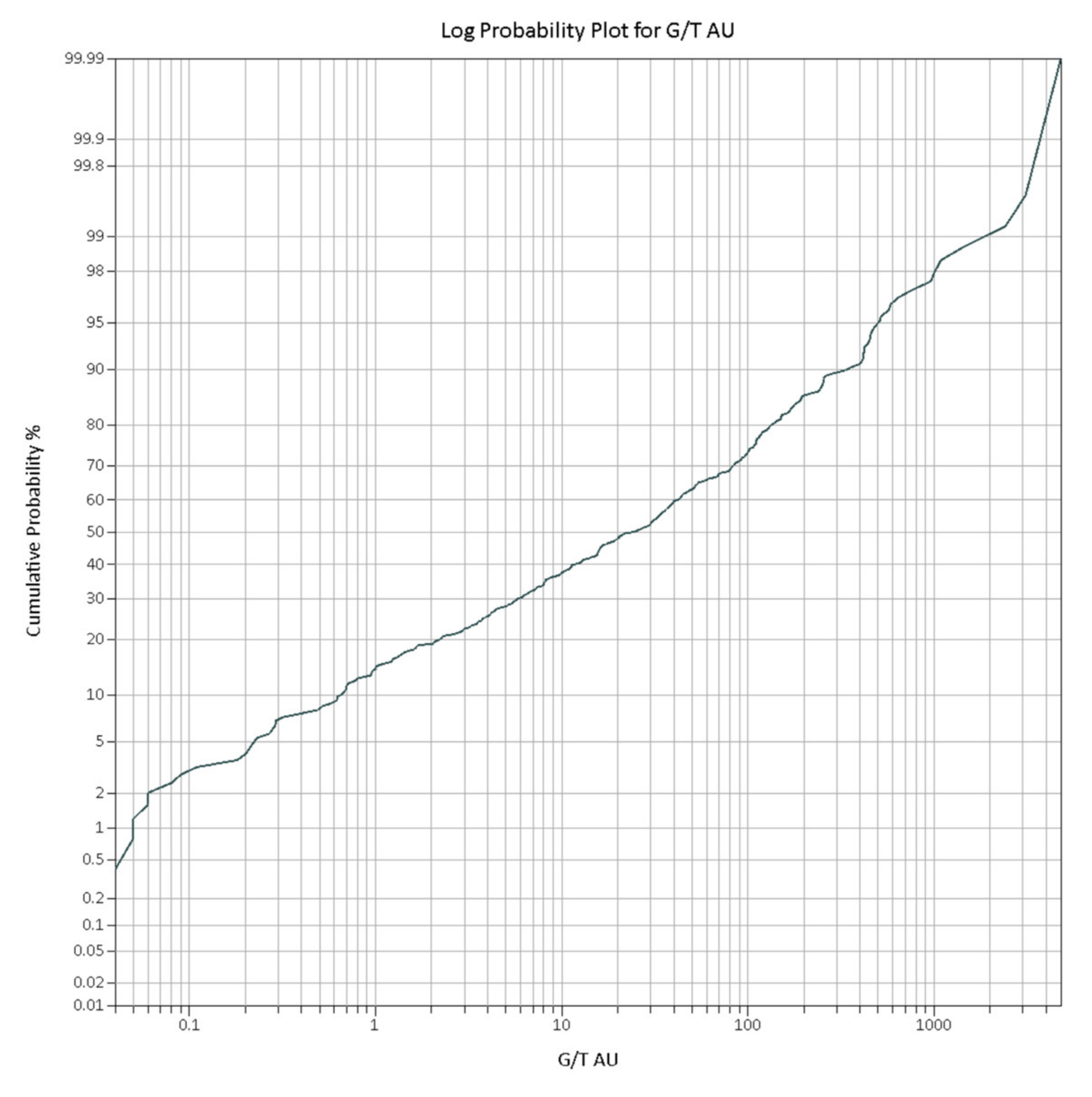
Gold particle populationVery coarse population >1000 µmLog-probability plot break point at approx. 1000 µm. Lower break point around 100 µm from MET/MIN data
Gravity recoverable goldVery highRaw data indicate dominant coarse gold (>200 µm) that has strong GRG potential
Gold association with galena flags potential concentration of galena within the gold gravity process. This was indeed noted during production.
Table 16. Representative sample mass for diluted mine faces and LV- and spur-only required to achieve precision of ±20% at the 68% confidence limits for different grade-liberation diameter scenarios. ROM: run of mine; BCOG: breakeven cut-off grade; CL: confidence limits; (c): clustered.
Grade TypeFace Grade (1)
(g/t Au)
LV Grade (1)
(g/t Au)
Liberation
Diameter (6)
(dℓAu—µm)
Face Diluted RSM (11,12) at 68% CL
(kg)
LV-Only
RSM (11,12) at 68% CL
(kg)
Very high grade (c)150 (2)74085055
Very high grade150 (2)74030004510
High grade39 (3)18585055
High grade (c)39 (3)1853000 (7)15035
ROM29 (4)15785065
ROM (c)29 (4)1571500 (8)305
ROM (c)29 (4)1573000 (7)20045
BCOG15 (5)8075085
BCOG (c)15 (5)80150010010
Low grade5 (9)15750107
Background grade4–6 (10)537555
Very low grade15375135
Low (spurs only)2.5-25055
(1) Grade based on 3.5 m minimum mining width and mean LV width of 0.7 m; (2) Very high grades encountered in upper levels; (3) Grade of MET1 (Table 12); (4) Reconciled Nick O’Time grade based on a variable mining width at a mean of 3.5 m; (5) Approximate breakeven cut-off grade during mine operation. dℓAu based on MET2 (Table 12). Additionally, typical grade of some lower mine areas; (6) Where appropriate, dℓAu used corrected XCT value (Table 12); (7) Clustering: dℓclus based on maximum cluster size from XCT; (8) Clustering: dℓclus based on half maximum value; (9) Typical grade of below 965 m RL; (10) Defined as the background gold grade (Table 3 and Figure 6), as diluted face grade of 3–4 g/t Au; (11) Optimum sample mass calculated via Poisson method. Any RSM below 5 kg, is reported as 5 kg; (12) ±20% at the 68% CL (N = 25 particles).
Table 17. Face RSM values for ultra-high grade cluster containing LV (0.7 m width) scenarios based on diluted face grade at 3.5 m width. RSM reported at a precision of ±20% at the 68% confidence limits and rounded to the nearest tonne. LV: laminated vein; ESD: equivalent spherical diameter.
Approx. Proportion of UHG ClustersLV Grade (g/t Au)Face Grade
(g/t Au)
1 Cluster (5)
ESD 12.2 mm
½ Cluster (5)
ESD 9.6 mm
⅓ Cluster (5)
ESD 8.4 mm
Representative Sample Mass
(t)
1%8015 (1)26139
1.5%140 (3)251896
2%15729 (2)1474
5%36565632
10%710125321
15%1050183211
19%1300225 (4)110.5
(1) BCOG; (2) ROM; (3) Mean LV grade; (4) Maximum recorded face grade; (5) Clusters are assumed to be spherical and based on agglomerated gold particle ESD.
Table 18. LV only RSM values for ultra-high-grade cluster containing LV (0.7 m width). LV: laminated vein; ESD: equivalent spherical diameter.
Approx. Proportion of UHG ClustersLV Grade (g/t Au)Face Grade
(g/t Au)
1 Cluster (2)
ESD 12.2 mm
½ Cluster (2)
ESD 9.6 mm
⅓ Cluster (2)
ESD 8.4 mm
Representative Sample Mass
5%365651 t525 kg350 kg
10%710125550 kg300 kg200 kg
15%1050183400 kg200 kg125 kg
18.5%1300225 (1)300 kg150 kg100 kg
(1) Maximum recorded face grade; (2) Clusters assumed to be spherical and based on agglomerated gold particle ESD.
Table 19. FSE values for the original production sampling protocol by vein domain for different grade-liberation diameter scenarios. The primary sample mass is based on a 0.7 m wide laminated vein (LV) and 2.8 m of spur vein. [c]: clustering.
DomainLV Grade
(g/t Au)
ScenariodℓAu
(µm)
Primary Sample Mass
(kg)
FSE
Laminated vein750Very high-grade LV3000 [c]5–7±11%
850±5%
140Mean LV to give mean face8505–7±10%
1500 [c]±16%
8015 g/t Au BCOG face8505–7±13%
1500 [c]±35%
155 g/t Au low grade face8505–7±32%
1500 [c]±48%
Spur vein2.5Mean2505–7±31%
Table 20. Duplicate evaluation of LV chip-channel samples.
Duplicate TypeExplanationNumberComponent
Error
Component Relative
Error
(RSV)
Proportion of Total
FieldChip-channel sample54Sampling±77%69%
CoarseLaboratory split after crushing37Preparation±51%30%
AssayAssayEst.Analytical±10%1%
Total--Total±92%100%
Table 21. Duplicate evaluation of spur vein chip-channel samples.
Duplicate TypeExplanationNumberComponent
Error
Component
Relative
Error
(RSV)
Proportion of Total
FieldChip-channel sample45Sampling±27%50%
CoarseLaboratory split after crushing37Preparation±25%44%
AssayAssayEst.Analytical±10%7%
Total--Total±38%100%
Note: the number of duplicate pairs is small compared to what would normally be considered optimal (>250 pairs). This is all that is available in this instance.
Table 22. Recommended PhotonAssay-based protocols to reduce the FSE and the effects of gold liberation by pulverising (gold loss/contamination).
ProtocolProtocol Steps
1
  • Dry and crush primary sample to P90 −2 mm
  • Rotary split 50%
  • PhotonAssay the entire 50% split
2
  • Dry and crush primary sample to P90 −2 mm
  • Take the entire sample for PhotonAssay
Table 23. Based on original grade control sample mass the FSE values for optimised sample preparation and PhotonAssay by vein domain for different grade-liberation diameter scenarios. The primary sample mass is based on a 0.7 m wide LV and 2.8 m of spur vein. Recommended sampling protocol as noted in Table 22. [c]: clustered gold values.
DomainLV Grade
(g/t Au)
ScenariodℓAu
(µm)
Primary Sample Mass
(kg)
Protocol 1: FSEProtocol 2: FSE
Laminated vein
(1 m × 0.7 m sample)
750Very high-grade LV8505–7±2–3%±0%
3000 [c]±6–7%±0%
140Mean LV to give mean face8505–7±6–7%±0%
1500 [c]±9–10%±0%
8015 g/t Au BCOG face8505–7±7–9%±0%
1500 [c]±11–13%±0%
155 g/t Au low grade face8505–7±17–20%±0%
1500 [c]±26–31%±0%
Spur vein
(3 m × 0.9 m samples)
2.5Mean2505–7±17–20%±0%
Table 24. Summary of RSM values for key scenarios.
LocationFaceLaminated Vein-Only
Upper mine levels
(>990 m RL)
UHG[c] >65 g/t Au<6 tUHG[c] >365 g/t Au<1 t
HG[c] 39 g/t Au150 kgHG[c] 185 g/t Au35 kg
ROM[c] 29 g/t Au30 kgROM[c] 157 g/t Au5 kg
Lower mine levels
(<990 m RL)
ROM[c] 29 g/t Au200 kgROM[c] 157 g/t Au45 kg
BCOG 15 g/t Au8 kgBCOG 15 g/t Au5 kg
LG 5 g/t Au 10 kgLG 15 g/t Au 7 kg
VLG 1 g/t Au13 kgVLG 5 g/t Au5 kg
UHG: ultra-high grade; HG: high grade; ROM: run of mine; BCOG: breakeven cut-off grade; LG: low grade; [c]: clustered.
Table 25. FSE values for the new optimised sampling protocols using PhotonAssay by vein domain for different grade-liberation diameter. 0.7 m wide LV and 2.8 m of spur vein. [c]: clustered gold.
DomainLV Grade
(g/t Au)
ScenariodℓAu or dℓclus
(µm)
Primary Sample Mass
(kg)
Protocol 1: FSEProtocol 2: FSE
Laminated vein
(1 m × 0.7 m sample)
750HG to give face grade of 150 g/t Au8507–14±2–3%±0%
3000 [c]±4–6%±0%
140Mean face grade of 29 g/t Au8507–14±4–6%±0%
1500 [c]±6–9%±0%
80BCOG face grade of 15 g/t Au8507–14±5–7%±0%
1500 [c]±8–11%±0%
15Low face grade of 5 g/t Au8507–14±12–17%±0%
1500 [c]±19–26%±0%
Spur veins (0.5 m samples)2.5Mean2501–2±0%±0%
Table 26. Cost data (Australia, October 2021) for the original and revised protocols and associated sample data precision. Analysis based on LV samples only.
ProtocolEstimated Cost per Sample
(A$)
Single Sample
Total Precision
Single Sample Laboratory to Assay PrecisionFour Sample Precision Based on a Single Development Round Informed by Four
Samples
Original6 kg sample to CL1000$85±92% (1)±51% (1)±46%
6 kg sample to SFA1000$100±92% (2)±50% (2)±46%
RecommendedProtocol 2: 11 kg sample to PA11000$210<±15% (3)<±5% (3)<±8% (3)
Protocol 1: 11 kg sample t PA5500$125<±25% (3)<±20% (3)<±13% (3)
CL: Cyanide leach 1 kg charge; SFA1000: Screen fire assay 1 kg charge; PA11000 & PA5500: PhotonAssay 11 kg and 5.5 kg charge. (1) Based on the global precision values given in Table 20; (2) Based on global precision values given in Table 20 with reduced analytical error for the screen fire assay; (3) Estimated values based on this study that may not be achieved in reality. A QC monitoring programme would be required to validate these estimates. Costs are based on generic values.
Publisher’s Note: MDPI stays neutral with regard to jurisdictional claims in published maps and institutional affiliations.

