Predicting the Logarithmic Distribution Factors for Coprecipitation into an Organic Salt: Selection of Rare Earths into a Mixed Oxalate

Abstract

Thermodynamic modelling of a leaching system that involves concurrent precipitation depends on an understanding of how the metals distribute into the precipitate before an assessment of solubility can be made. It has been suggested in the past that a pair of rare earths (A and B) in solution will separate from each other by oxalate precipitation according to a logarithmic distribution coefficient ($\mathsf{\lambda }$), determined by the kinetics of the precipitation. By contrast, the present study hypothesises that $\mathsf{\lambda }$ may be approximated from thermodynamic terms, including the solubility product (K_Sp) of each rare earth oxalate and the stability constant (${\mathsf{\beta }}_1)$ for the mono-oxalato complex of each rare earth. The proposed model was used to calculate $\mathsf{\lambda }$ between pairs of rare earths. An experimental study was conducted to determine $\mathsf{\lambda }$ between selected pairs using homogenous precipitation through the hydrolysis of an oxalic acid ester, with fairly close agreement to the values under the proposed model. Though this model requires more thorough testing, as well as application to other organic salts, it may provide insight into distribution factors of a precipitate formed by a sequence of organic complexes.

1. Introduction

In rare earth extraction, a common technique for overcoming the poor solubility of rare earth minerals is to transfer the rare earth ions into a more stable solid. In sulfuric acid cracking, for example, the rare earths are transferred into solid sulphates. In caustic conversion, the rare earths are put into hydroxides. In more recent studies, minerals of rare earth phosphates have been dissolved in oxalic acid, while the rare earths concurrently precipitate as rare earth oxalates [1,2]. In each of these techniques, an effective transfer of the rare earths depends on each rare earth having a lower solubility or a higher stability in the destination compound.

The way that rare earths distribute into an oxalate precipitate has not been modelled, beyond describing the results of specific experimental conditions. This is despite oxalate coprecipitation being a common technique in a broad range of areas. Oxalate coprecipitation is a standard method for producing precursor powders that are calcined into mixed metal oxides. Examples in the literature abound, such as precursors for magnetic materials [3], piezoelectric oxides [4], superconducting materials [5,6] and alloys [7]. It is also used to separate rare earths and actinides from other ions in solution by precipitation. Breakdown of rare earth minerals such as monazite are often done in extreme conditions [8] that dissolve impurity ions along with the rare earths. The very low solubility of rare earth and actinide oxalates enables an isolation of rare earths from mixed solutions [9].

The most advanced modelling of oxalate co-precipitation appears to have come from experiments to separate rare earths from each other in controlled precipitation. Oxalic acid was generated homogeneously throughout the solution by hydrolysis of dimethyl oxalate, in order to minimize concentration gradients within the solution and allow separations closer to those predicted by solubility [10]. Feibush, Rowley and Gordon [11] found, however, that the separations were much lower than predicted, according to solubility for the rare earths tested in their study. There remained no method to predict the separation from fundamental terms, and the techniques for oxalate coprecipitation more generally appear to be based on trial and error.

Feibush, Rowley and Gordon [11] did find that the precipitation between pairs of rare earth oxalates follows a Doerner–Hoskins or logarithmic distribution coefficient. Such a distribution assumes that the precipitating solid does not re-order its whole self to be in equilibrium with the solution; rather, the precipitated surface is in equilibrium with the solution and once precipitated it forms an unchanging substrate for the next surface layer [12]. Doerner and Hoskins were the first to describe this running equilibrium mathematically [13]. It can be described between concentrations of rare earth ions [A] and [B] by Equation (1).

$$\frac{d\left[A\right]}{d\left[B\right]}=\lambda \frac{\left[A\right]}{\left[B\right]}$$

(1)

Here, $\frac{d\left[A\right]}{d\left[B\right]}$ is the ratio of the concentration of A to B lost from the solution in an infinitesimal increment, or, in other words, precipitated onto the surface in an infinitesimal increment. The letter $\lambda$ signifies the logarithmic distribution coefficient. This expression can be integrated to give Equation (2).

$$ln\frac{\left[A\right]final}{\left[A\right]initial}=\lambda ln\frac{\left[B\right]final}{\left[B\right]initial}$$

(2)

Doerner and Hoskins [13] did not attempt to correlate the coefficient to fundamental terms, probably in the knowledge that different salts may be governed by different terms. Feibush, Rowley and Gordon [11] suggested that with rare earth oxalates, the coefficient should be the ratio between the square roots of the solubility products of the pure rare earth oxalates (square root because each unit of rare earth oxalate has two rare earth ions), as shown in Equation (3).

$$\lambda \cong \frac{\sqrt{K_{Sp,A}}}{\sqrt{K_{Sp,B}}}$$

(3)

This equation is based on $K_{Sp, A}$, as the solubility product for the equation shown in Equation (4).

$$A_2{\left(C_2{O}_4\right)}_3\to 2A^{3+}+3C_2{O}_4{}^{2-}$$

(4)

Their experiments, however, showed that the experimental values of the coefficients, while being logarithmic in nature, were far from what was predicted by solubility in the form of Equation (3). Equation (3) does not form a basis in the present study for further development of a model.

Some more recent work on the solubility of rare earth oxalates has determined that the saturated concentration of rare earth A in a solution of concentrated oxalic acid is determined by Equation (5) [14].

$$\left[A_{total}\right]=\frac{\sqrt{K_{Sp,A}}}{{\gamma }_3}{\left(a_{C_2{O}_4{}^{2-}}\right)}^{-3/2}+\frac{\sqrt{K_{Sp,A}}{\beta }_{1,A}}{{\gamma }_1}{\left(a_{C_2{O}_4{}^{2-}}\right)}^{-1/2}$$

(5)

In Equation (5), ${\beta }_{1,A}$ is the equilibrium constant for the reaction in Equation (6), with the subscript number denoting the number of oxalates in the complex formed. The expression for ${\beta }_{1,A}$ is shown in Equation (7), where $a$ is the activity of the species denoted as subscript. The symbol ${\gamma }_1$ is the activity co-efficient for the rare earth mono-oxalato complex, and ${\gamma }_3$ is the activity co-efficient for the free rare earth ion, the subscript based on the magnitude of the charge.

$$A^{3+}+C_2{O}_4{}^{2-}\to A{C}_2{O}_4{}^{1+}$$

(6)

$${\beta }_{1,A}=\frac{a_{A{C}_2{O}_4{}^{1+}}}{a_{A^{3+}}{a}_{C_2{O}_4{}^{2-}}}$$

(7)

It can be seen in Equation (5) that the total concentration of rare earth A is made up of two main species, the free or weakly-complexed rare earth ion in the first term, and the mono-oxalato complex in the second term. In one sense, Equation (5) represents the saturated concentrations of each of these species in the particular system. The challenge from a theoretical point of view is how a model of precipitation can be constructed if there are complexes present. For example, the precipitate may be formed from a sequence of complexation reactions, where the mono-oxalato complex is the precursor to the precipitate, rather than the free rare earth ion.

2. Materials and Methods

Rare earth oxides at a minimum of 99.9% purity were obtained from Treibacher Industries in Austria, along with certificates of assay. Dimethyl oxalate (99%) was obtained from Alfa Aesar, and diethyl oxalate (99%) from Sigma Aldrich. Analytical grade hydrochloric acid was used. Brand-new Duran 100 mL conical flasks were used for each experimental flask.

The method underwent considerable development. In the original method, each conical flask was initially weighed. To each conical flask was added at least two, but up to six, rare earth oxides. The amount of each rare earth oxide added was determined by a random number generator in Microsoft Excel, to be an amount between 0.00 and 0.10 g. As close to this number as possible was weighed and added to the flask. Hydrochloric acid was then added to dissolve the rare earth oxides into chlorides until a clear solution was obtained. The flask was then heated on a hotplate to evaporate the remaining hydrochloric acid and water, and leave a precipitate of rare earth chlorides. To the flask was added about 100 g of deionized water. The mass of dimethyl oxalate (DMO) required for a complete precipitation was calculated, and a fraction of this was chosen at random, weighed and added to the flask. The solution was swirled until all the dimethyl oxalate was dissolved. This also had the effect of dissolving any residual rare earth particles (either difficult crystals of chlorides or hydroxides). A stopper was placed in the opening of the flask. The flask was submerged in a water bath at 25 °C and left for a week. One week was chosen based on informal testing—after about four days, the solution could be decanted into another vessel without further precipitation. A sample of the solution was taken by pipette and diluted with hydrochloric acid (0.1 M), for analysis by ICP-AES. The density of the solution was checked to be 1 g/mL.

This method produced internally consistent results between yttrium, erbium and thulium. However, in the case of lanthanum or neodymium, the initial stages of the precipitation proceeded without the involvement of one or more of the elements. To minimize the impact of this initial precipitation, a higher initial concentration of rare earths was used so that the final concentration covered a greater range of concentration. Also, to minimize errors of measurement of the initial solution, a stock solution was prepared for use in every conical flask. To allow a slower, more gradual precipitation, diethyl oxalate (DEO) was chosen as the oxalic acid ester. This appears to have a slower rate of hydrolysis than dimethyl oxalate.

About 5 g of each of lanthanum, neodymium and yttrium oxides were dissolved together in the one flask in hydrochloric acid, and evaporated to rare earth chlorides. Deionized water and 1 mL of hydrochloric acid (10 M) was added to a total of 1000 g. The 1 mL of hydrochloric acid was to dissolve any rare earth hydroxides that may be present. The pH was not measured, since the acidity during the experiment increases as more of the oxalic acid ester hydrolyses, so that a constant pH could not be maintained without the use of a buffer that may complex the rare earth ions. To each 100 mL conical flask was added to about 100 g of rare earth solution and a weighed amount of diethyl oxalate solution. The diethyl oxalate was added by a glass dropper, as diethyl oxalate can be a solvent of plastic. A sample of the solution was taken by pipette and diluted with hydrochloric acid (0.1 M) for analysis by ICP-AES. The density of the solution was checked to be 1 g/mL.

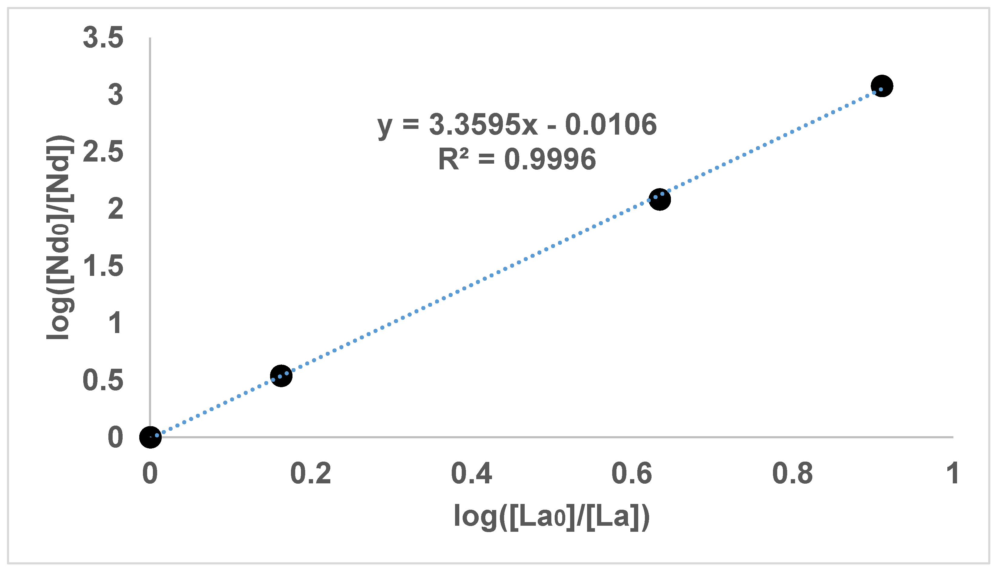
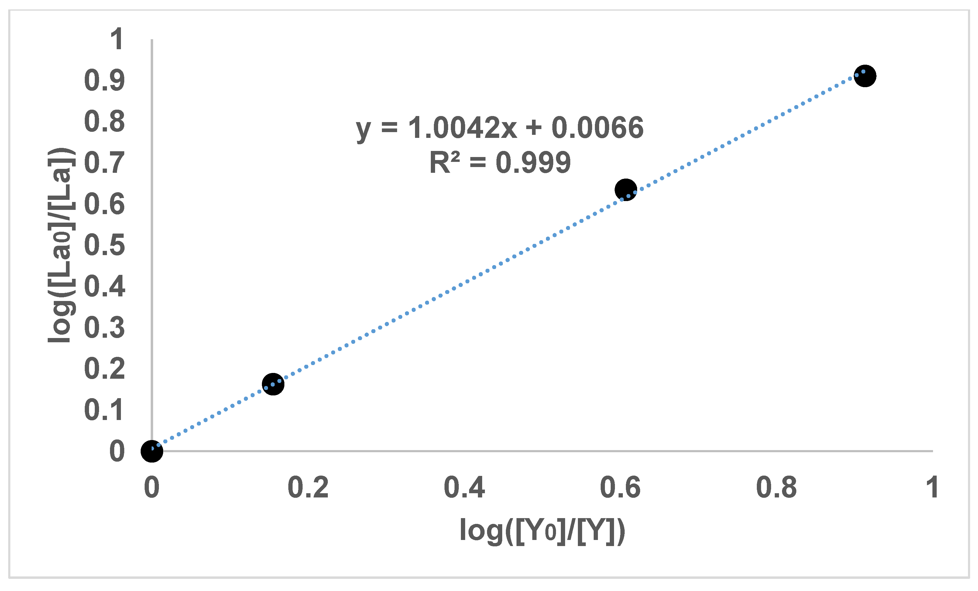
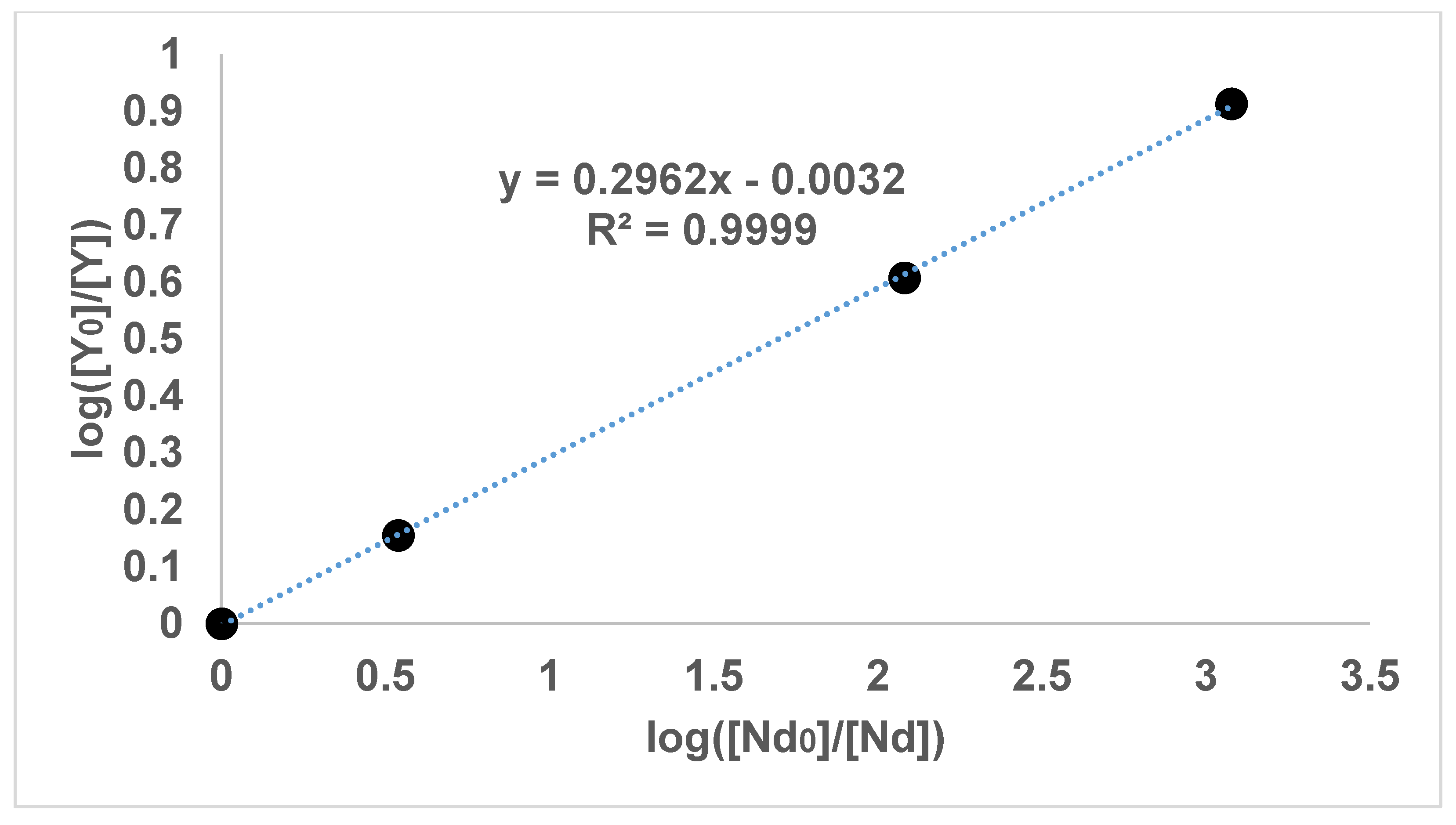
It was decided to plot the results between two rare earths from every experimental vessel on the one graph. The graph was based on Equation (2), so that the logarithm of the quotient of the starting concentration and final concentration was plotted on an axis for one element, while the same was plotted on the other axis for the other element. In this way, the slope of the graph should give the logarithmic distribution coefficient. The reason why this graphical method was chosen rather than tabulating the coefficient for each experiment was because the graph allows checks of internal consistency. Firstly, the line of best fit should be passing through the origin. This is because any constants of integration would be cancelled out in the integration of Equation (1) to Equation (2). Secondly, the ratios between a pair should be expressible in terms of the others; for example, pairs in a triplet should multiply to one, as illustrated by Equation (8):

$$K_{\frac{A}{B}}=K_{\frac{C}{B}}\times K_{\frac{A}{C}}$$

(8)

This is because the logarithmic distribution coefficient should be consistent between a pair regardless of how many rare earths are in the system.

3. Results

Table 1. Identity of solution components and masses for each experiment.

Experiment Number	Solution Components	Solution Mass, g	Ester	Ester Mass, g	Total Mass, g
1	La, Pr, Nd, Y, Er, Tm	$100.00$	DMO	-	$100.00$
2	Y, Er, Tm	$100.16$	DMO	-	$100.16$
3	La, Pr, Nd, Y, Er, Tm	$100.01$	DMO	-	$100.01$
4	Y, Er, Tm	$100.04$	DMO	-	$100.04$
5	Y, Er	$100.84$	DMO	-	$100.84$
6	La, Nd, Y	$102.62$	DEO	$2.04$	$104.66$
7	La, Nd, Y	$102.24$	DEO	$4.20$	$106.45$
8	La, Nd, Y	$102.65$	DEO	$1.05$	$103.70$
9	La, Nd, Y	$101.50$	DEO	$3.15$	$104.65$

shows which rare earths and ester were in each experimental vessel or conical flask, as well as the solution masses used to calculate the initial concentration. The first five experiments used the original experimental method. In this procedure, the total solution mass was weighed after the rare earth chlorides and dimethyl oxalate were dissolved. The last four experiments used the stock solution. In this method, the assayed stock solution was weighed into the conical flask and then the addition of diethyl oxalate was weighed.

Table 2. Initial and final solution concentrations for each experiment.

Experiment Number		La (ppm)	Pr (ppm)	Nd (ppm)	Y (ppm)	Er (ppm)	Tm (ppm)
1	Initial	$486$	$880$	$183$	$603$	$450$	$883$
	Final	$289$	$493$	$90$	$508$	$340$	$621$
2	Initial	-	-	-	$802$	$661$	$600$
	Final	-	-	-	$323$	$170$	$168$
3	Initial	$549$	$115$	$920$	$430$	$191$	$514$
	Final	$199$	$15$	$66$	$198$	$57$	$158$
4	Initial	-	-	-	$589$	$493$	$385$
	Final	-	-	-	$330$	$202$	$163$
5	Initial	-	-	-	$962$	$274$	-
	Final	-	-	-	$667$	$150$	-
6	Initial	$5603$	-	$4831$	$3681$	-	-
	Final	$1300$	-	$40$	$910$	-	-
7	Initial	$5488$	-	$4732$	$3606$	-	-
	Final	$BDL$	-	$BDL$	$BDL$	-	-
8	Initial	$5656$	-	$4877$	$3717$	-	-
	Final	$3885$	-	$1410$	$2600$	-	-
9	Initial	$5542$	-	$4779$	$3642$	-	-
	Final	$680$	-	$4$	$445$	-	-

shows the calculated initial concentrations and the measured final concentrations in each experimental vessel. In Experiment 7, too much diethyl oxalate was added, and complete precipitation occurred, so that the rare earths were below the detection limit (BDL).

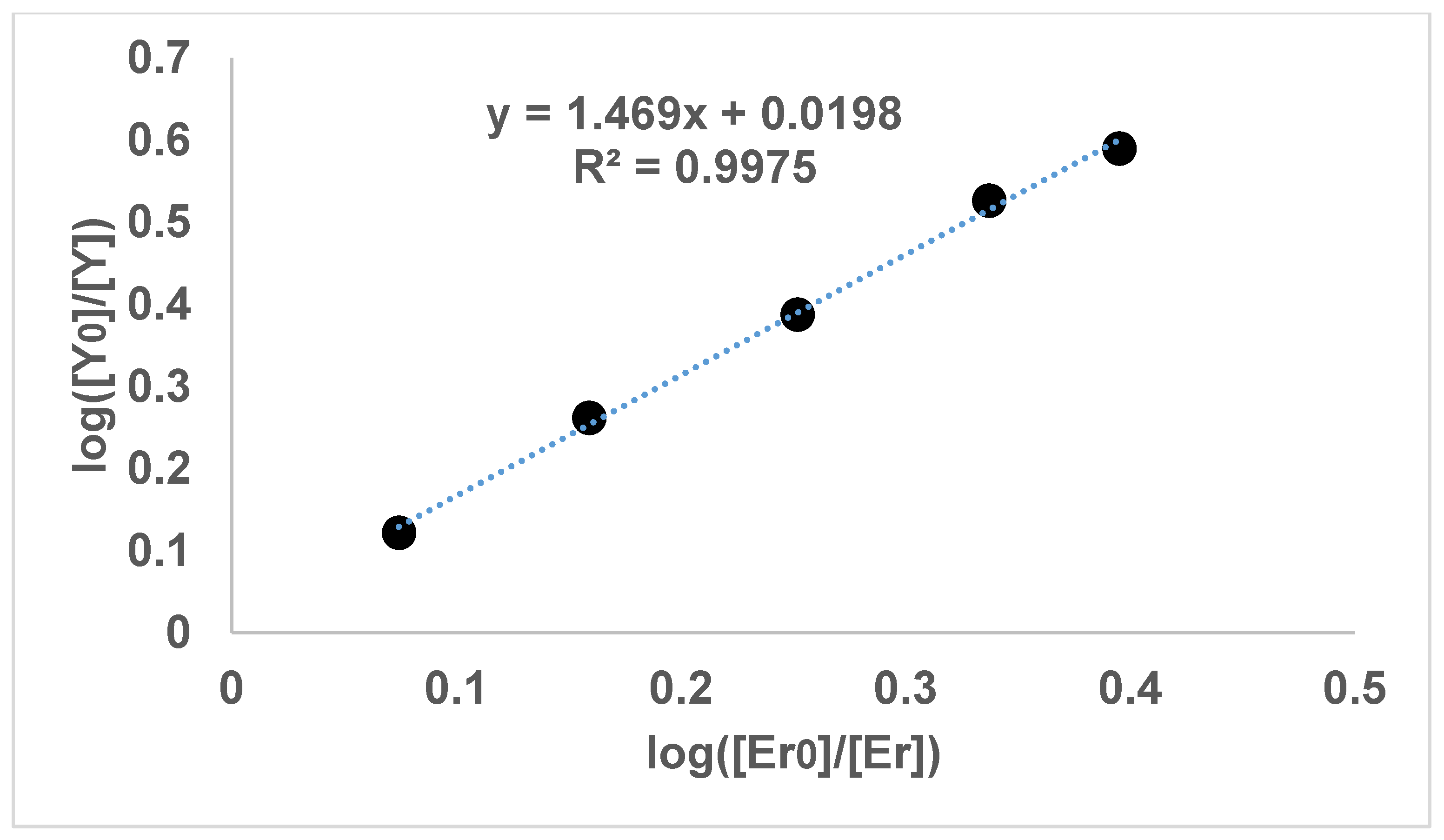
Figure 1, Figure 2 and Figure 3 show the results of the experiments with diethyl oxalate and concentrations of lanthanum, neodymium and yttrium. In addition, Figure 4 shows the result of the experiments with dimethyl oxalate and yttrium and erbium, in which the intercepts were also small, so that the use of diethyl oxalate was not required. The graphical results involving thulium also had a small intercept but are not shown here, as no thermodynamic data for thulium could be found for correlating the slopes of the graphs.

It can be seen in Figure 1, Figure 2, Figure 3 and Figure 4 that the results have an internal consistency, with the lines of best fit having an intercept close to the origin. Also, when the slopes of Figure 1, Figure 2 and Figure 3 are multiplied together as a triplet, the product is very close to one, indicating another internal consistency. The data points also fit fairly closely to a straight line, although deviations will appear to be diminished somewhat by the logarithmic axes.

It would have been preferable to have had a greater number of data points on each graph. However, each data point comes from a separate experimental vessel, and there was no exclusion of outliers, apart from Experiment 7, in which the precipitation was complete. In terms of repetition, in one sense each data point on the one graph is a repetition of the same separation, although repetition of the same specific conditions would also provide greater confidence. Overall, it seems that the slope values in Figure 1, Figure 2, Figure 3 and Figure 4 can be described as the logarithmic distribution coefficient ($\mathsf{\lambda }$), found experimentally.

4. Discussion

Given that Equation (3) did not describe the distribution coefficient $\mathsf{\lambda }$ [11], and that it is based on the solubility of the free or weakly-complexed rare earth ion, an alternative basis for describing $\mathsf{\lambda }$ was needed. It was hypothesized that the precipitation was governed by the energy difference between the solid rare earth oxalate and the mono-oxalato complex in Equation (9).

$$A{C}_2{O}_4{}^{1+} \leftrightarrow 0.5 A_2{\left(C_2{O}_4\right)}_3$$

(9)

Equation (10) was posed as a way to describe $\mathsf{\lambda }$, because it represents the ratio of the equilibrium constants for Equation (9), which in turn is based on Equations (4) and (6). It also approximates the ratio of the saturated concentrations of the mono-oxalato complexes of each rare earth in question on the basis of Equation (5), assuming that the activity coefficient ${\gamma }_1$ is similar between rare earths. The term in Equation (5) for the free or weakly-complexed rare earth ion was neglected, as it seemed unlikely that solid rare earth oxalates would form directly from this simple species.

Equation (10) was used to calculate theoretical values in

Table 3. Comparison between theoretical and experimentally obtained values for the logarithmic distribution coefficient.

Pair	Theoretical	Experimental
Nd/La	3.25	3.36
La/Y	0.96	1.00
Y/Nd	0.32	0.30
Y/Er	1.47	1.47

. The experimentally found values match these theoretical values fairly closely.

$${\mathsf{\lambda }}_{\frac{\mathrm{B}}{\mathrm{A}}}\cong \frac{\sqrt{{\mathrm{K}}_{\mathrm{Sp},\mathrm{A}}}{\mathsf{\beta }}_{1,\mathrm{A}}}{\sqrt{{\mathrm{K}}_{\mathrm{Sp},\mathrm{B}}}{\mathsf{\beta }}_{1,\mathrm{B}}}$$

(10)

The theoretical values for $\mathsf{\lambda }$ were calculated using Equation (10) on the results obtained by Chung, Kim, Lee and Yoo [14], shown in

Table 4. Solubility products [14], equilibrium constants [14] and their products $\sqrt{K_{Sp} }{\beta }_1$.

Element	$\mathbf{Solubility}\mathbf{Product},{\mathit{K}}_{\mathit{S}\mathit{p}}$	$\mathbf{Equilibrium}\mathbf{Constant},{\mathit{\beta }}_1$	$\sqrt{{\mathit{K}}_{\mathit{S}\mathit{p}}}\mathit{·}{\mathit{\beta }}_1$
Y	$5.1\times {10}^{-30}$	$2.3\times {10}^7$	$5.2\times {10}^{-8}$
La	$6.0\times {10}^{-30}$	$2.2\times {10}^7$	$5.4\times {10}^{-8}$
Nd	$1.3\times {10}^{-31}$	$4.6\times {10}^7$	$1.7\times {10}^{-8}$
Sm	$4.5\times {10}^{-32}$	$3.2\times {10}^7$	$6.8\times {10}^{-9}$
Eu	$4.2\times {10}^{-32}$	$3.3\times {10}^7$	$6.8\times {10}^{-9}$
Gd	$4.25\times {10}^{-32}$	$3.5\times {10}^7$	$7.2\times {10}^{-9}$
Dy	$2.0\times {10}^{-31}$	$4.9\times {10}^7$	$2.2\times {10}^{-8}$
Er	$9.0\times {10}^{-31}$	$8.0\times {10}^7$	$7.6\times {10}^{-8}$

. The theoretical values for $\mathsf{\lambda }$ for the range of rare earths for which data is available are shown in

Table 5. Calculated logarithmic distribution coefficients (precipitation of the element in the horizontal row for every one of the elements in the vertical column).

Element	La	Nd	Sm	Eu	Gd	Dy	Er
Y	$0.96$	$3.1$	7.7	7.7	7.2	2.4	0.68
La		$3.25$	7.9	8.0	7.5	2.5	0.71
Nd			2.4	2.5	2.3	0.76	0.22
Sm				1.0	0.94	0.31	0.09
Eu					0.94	0.31	0.09
Gd						0.33	0.10
Dy							0.29

.

The reason why Equation (10) should approximate $\mathsf{\lambda }$ is a conundrum. Firstly, the most abundant form of each rare earth will be the mono-oxalato complex only in a concentrated solution of oxalic acid according to Equation (5). In the present case, a hydrolyzing ester will only produce a very dilute concentration of oxalic acid before precipitation occurs, meaning that the most abundant form of rare earth in solution will be the free or weakly-complexed ion according to Equation (5). This implies that the measured final concentrations are mainly made up of free or weakly-complexed rare earth ions, and that the model is still a relation between the concentration of these ions and the fractions on the surface of the precipitate. Yet, according to Equation (9), the free rare earth ion is not involved in that equilibrium directly.

Nor is there an obvious kinetic argument, as a higher stability of mono-oxalato complex will cause less precipitation into the solid oxalate compound under this particular model. It would perhaps be expected that a higher concentration of mono-oxalato complexes would lead to a higher rate of collisions leading to precipitation.

The notion of a stepwise formation of organic complexes into an organic salt also does not yield an adequate explanation. The concentration of the mono-oxalato complex of each rare earth would be determined by the stability constant in Equation (7), as well as the activity fraction of the free rare earth ion. Adding the chemical equations for the formation of the mono-oxalato complex (Equation (6)), and the formation of the precipitate from the mono-oxalato complex (Equation (9)) merely yields Equation (4), which represents the solubility product.

The system is behaving as though the ratio of the concentrations of the mono-oxalato complex of each rare earth is the same as that for the free rare earth ions. It may be conjectured that Equation (6) for the formation of the mono-oxalato complex is not attaining equilibrium before precipitation is occurring. It is possible that this may be connected to the very low concentration of oxalic acid and the very low solubility of the oxalate precipitate. Overall, it remains difficult to explain the model from kinetic and thermodynamic principles.

5. Conclusions

It was found that the logarithmic distribution co-efficient $\mathsf{\lambda }$ for precipitation between a pair of rare earths was fairly close to the ratio of the equilibrium constants for the step from mono-oxalato complex to the rare earth oxalate salt. This model relates the total concentration of rare earths (mostly free rare earth ions) to the fractions precipitating into the solid, so it is unclear why only the last step of the precipitation counts for $\mathsf{\lambda }$. There appears to be no simple kinetic explanation either, with $\mathsf{\lambda }$ being derived from thermodynamic terms, and the curious result that a higher stability of mono-oxalato complex results in less precipitation.