Mapping Suburbs Based on Spatial Interactions and Effect Analysis on Ecological Landscape Change: A Case Study of Jiangsu Province from 1998 to 2018, Eastern China

Abstract

As the transitional area between urban and rural areas, land-use change in suburbs is drastic, which generates negative effects on the ecological environment. However, the identification of the suburbs remains controversial. Usually, the density of the population and residential land is referenced, and the close spatial interactions between urban areas and suburbs are generally neglected. To fill this research gap, this study adopts a case study method to map the suburbs of Jiangsu based on estimating the spatial interactions. First, a regression model is built to estimate the population distribution. Second, a radiation model is utilized to evaluate the spatial interaction at a grid level. After the main urban area is identified based on the high density of the population and construction land, the interaction strength between the main urban grid and other grid areas is calculated, and the grids that share high values of interaction strength with urban grids are identified as suburban areas. Finally, the suburbs of Jiangsu in 1998 and 2018 are mapped, and the ecological landscape pattern metrics are used to verify the effects of suburban expansion. As a result, the suburban expansion of Jiangsu over the 20 years was significant, and the effects of suburban expansion on ecological land fragmentation were evident. On the basis of the results, the enlightenment of mapping suburbs on ecological landscape planning is discussed.

1. Introduction

Mainland China has experienced unprecedented socioeconomic development since the reform and opening-up in 1979. The urbanization of China retains a rapid pace, which increased from 17.92% in 1978 to 59.60% in 2018, and scholars predict it will reach 70% in 2035 and 75% in 2050 [1]. During urbanization, many people migrate from rural to urban areas; hence, the aggregation of people, industrial development, and urban construction create large demands for land use. Existing studies have proven that the expansion of urban land mainly sacrifices rural land, especially cropland [1,2,3], which produces negative effects such as ecological degradation, water and land loss, and soil pollution [3,4,5,6,7,8]. As one of the basic characteristics of urbanization, urban land expansion has garnered much attention, and studies have focused on land transition monitoring, effects analysis, and mechanism identification [9,10,11,12]. However, discussions on suburban development and its subsequent effects remain insufficient.

Suburbs are areas that are adjacent to the main urban area and are characterized by mixed land use that includes urban and rural areas, with a mediate construction and population density as compared with urban and rural areas and accessible commuting distance to a city [13,14]. The contemporary origins of suburbs are from the UK, USA, and Australia and now extend worldwide in both developed and developing countries [15]. The driving forces of suburban development in developed and developing countries are different. For example, suburban development in the UK was observed in the late 18th century due to the rich middle classes resettling in the outskirts of London [16]. From this perspective, suburban development has usually been studied under the framework of suburbanization; low density and car dependence are historically the main characteristics of such suburban areas [17,18]. Suburban development in developing countries such as China is mainly caused by urbanization and urban expansion. One the one hand, the aggregation of people in urban areas creates a large construction land demand for industrial development and residential land. On the other hand, the pressure produced by the high price of renting and purchasing flats in the city drives some people to live in comparatively cheap suburbs, which also prompts the land-use change of suburban areas. Despite the differences in suburban development in developed and developing countries, land transition, especially the transition from rural to urban land, is a common feature that has negative effects on ecological environment protection, historical town preservation, and cropland guarantees [19,20,21]. Therefore, mapping and tracking the changes in suburbs and analyzing their effects on land-use and landscape change are of great significance.

Forsyth [13] reviewed the studies on identifying suburbs and concluded it is important because it is the premise of taking actions in suburban planning and it provides definitions and features that empirical research requires. Existing studies on mapping suburbs are mainly based on the density of residential land or population. However, it is difficult to set an exact density standard to distinguish between urban, suburban, and rural areas. Additionally, suburbs share close social, economic, and spatial interactions with urban areas [22,23], which are rarely considered in existing studies on mapping suburban boundaries. By adopting a case study method, this study first interprets Landsat series data to extract the land-use information of Jiangsu in 1998 and 2018; then, this study simulates the population distribution at a 30 m resolution, through which a radiation model is applied to estimate the spatial interactions at a grid scale. For the interaction strength, the grids are classified into main urban, suburban, and rural areas. By mapping the suburbs, suburban expansion is traced, and its effects on land use, especially ecological landscape changes, are analyzed. The main goals of this study are (1) to map the suburban areas by considering their spatial interactions, (2) to analyze the ecological landscape change, and (3) to offer possible suggestions for suburban management and planning to aid ecological landscape protection. The structure of this study is as follows: Following the introduction in Section 1; in Section 2 we present the literature review section, which assesses studies on mapping suburbs and ecological landscape change analyses; Section 3, features the introduction of the study area; followed by the methodology in Section 4; in Section 5 we present detailed descriptions about the results of the analyses; in Section 6, we discusses the findings and the implications; and finally, in Section 7, we state concludes with the results and discuss the highlights and significance.

2. Literature Review

2.1. Measures of Mapping Suburbs

Although the definition of a suburb has never been standardized, a suburb is usually thought to be a mixed area of urban and rural lands that is adjacent to a city and within commuting distance of that city. According to existing studies, measurements of mapping suburbs are mainly based on administrative, spatial, social, and functional dimensions. The definitions and relevant applications are shown in

Table 1. Examples of defining suburbs based on different dimensions.

Dimension	Indicator	Explanation	Application
Administrative	Administrative boundaries	Residential municipalities such as towns close to a city	Forman [24] and Banzhaf et al. [25] identified urban and suburbs based on administrative municipalities.
Spatial	Location	Adjacent to the city; within the commuting distance of the city	Clapson and Hutchison [18] defined suburbs as areas that were between the town center and the countryside but within accessible distance. Johnson et al. [26] pointed out living in suburbs is founded on mobility since suburbs are on the periphery of the city.
	Density	Residential land or population density	Gordon and Janzen [27] utilized population density based on census data to identify the urban, suburban, and rural areas of Canada. Heris [28] identified the suburbs in the USA by estimating the housing density.
	Spatial activity	Journey-to-work data	Gordon and Janzen [27] identified the core city and its suburbs according to the proportion of walking and cycling transportation based on people’s journey-to-work data.
Social	Social attributes	Social attributes such as classes, races, and ethnicities of residents that distinguish cities and suburbs.	Gober and Behr [29] found that race and ethnicity were the most important elements to distinguish the core city and suburbs in the USA. Paccoud and Mace [30] discussed the social upscaling of Outer London from 2001 to 2011.

.

Most studies utilize at least two dimensions together to implement identification, and location and density features are the most commonly adopted methods to identify suburbs. However, there is criticism that these methods oversimplify the urban form and depend on arbitrary classifications [31]. To improve the accuracy of identifying suburbs, this study uses the traditional method of population and construction land density to determine the main urban areas and refers to urban–suburban interaction to map suburbs.

2.2. An Effect Analysis of Suburban Expansion

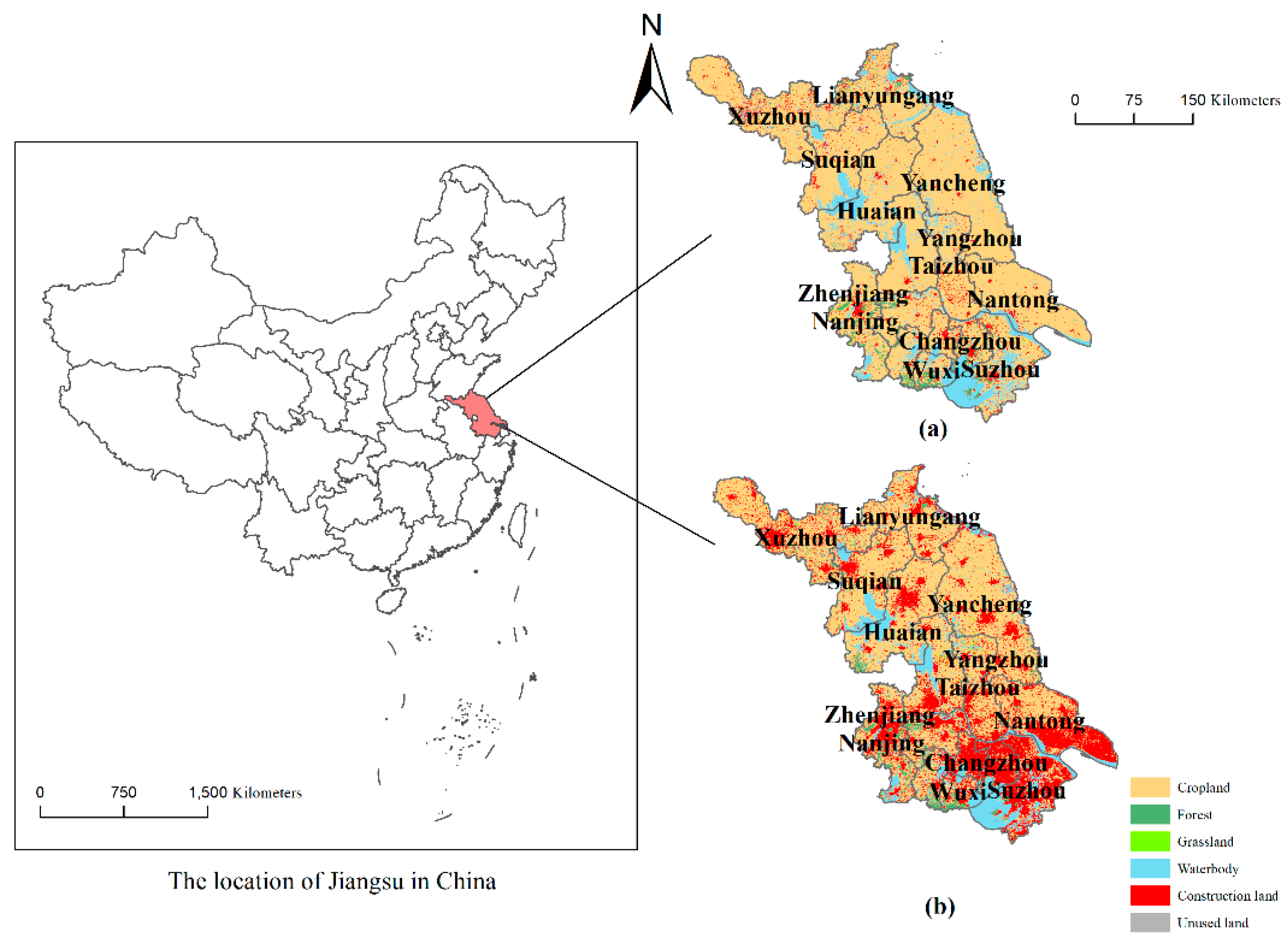
The effects of urban expansion have been discussed widely in existing studies, of which the urban sprawl catches most concerns. The modern term “sprawl” was first proposed by city planners in the early 20th century and was proven to be related to transportation development and an increase in income [32]. Later, the phenomenon of urban sprawl received much attention. “Urban sprawl” denotes an unplanned and uneven pattern of urban development that usually leads to inefficient utilization of land resources [33]. Despite the many studies on urban sprawl, little attention has been paid to suburban expansion. The measurement of urban expansion usually relies on measuring the land transition that occurs beyond the built-up urban area, including low density edge expansion and leapfrog growth [34]. However, the boundaries of suburbs are usually larger than the scope of urban areas, and the land-use change in suburbs includes urban expansion, and also rural construction land increment; hence, the effective areas of suburbs expand the outline of continuous urban construction land, which is insufficiently discussed.

Several studies have proven the effects of suburban expansion on land fragmentation and ecological conservation. For example, Novak and Wang [35] analyzed the impacts of suburban sprawl on Rhode Island’s landscape. Specifically, they found that the land transition in the study area contributed to the scarification of forest land and that ecological connectivity also declined. By applying U.S. census data, Radeloff et al. [36] extracted housing density data and analyzed the environmental impacts of suburban and rural sprawl. The authors concluded that suburban sprawl was related to forest fragmentation. Lian et al. [37] utilized time series data to analyze the spatial-temporal patterns of farmland loss and fragmentation in urban, suburban, and exurban areas under the background of rapid urbanization. Wang et al. [38] analyzed the correlation between suburban development and ecological deterioration. As a conclusion, the authors found that suburban growth caused changes in ecological and environmental quality. In summary, existing studies on the effect of suburban expansion, from the perspective of land transition, have focused on a single land-use type such as forest land or farm land, while ecological effect analyses of suburban growth have mainly focused on a single aspect of the environment, such as the atmosphere or water [39,40,41].

The essence of suburban expansion includes a complex land transition process. First, the land-use structure changes. The identification expansion, cropland land, and other types of rural land, such as forest and grassland, transition into urban construction land. Additionally, rural construction land, including rural settlements and industry construction land located in the countryside, also create a large land demand. Second, suburban expansion also has effects on the landscape, especially the ecological landscape. Although there is no common agreement on the definition of “ecological land”, most scholars define it using the framework of ecosystem services, including supporting, provisioning, regulating, and cultural services [42]. In addition, new works to study ecosystem services, such as the European Biodiversity Strategy to 2020, have adopted a perspective of biodiversity, and classified the terrestrial ecosystems into urban, cropland, grassland, woodland and forest, heathland and shrub, sparsely vegetated land, and wetlands [43]. The components of ecological land differ in different studies. In this study, the ecological land is defined as a kind of land that provides ecological services and goods, which is distinguished from construction land [44]. The land-use types of land classification include cropland, forest (including orchard), grassland, waterbody, construction land, and unused land. Cropland, forest, grassland, and waterbody are classified as ecological land due to the importance of their ecological functions and services. Ecological landscape refers to the landscape of ecological land.

By mapping the scope of the main urban, suburban, and rural areas, this study adopts the landscape pattern metrics to describe changes in suburban ecological landscape patterns. To verify the importance of mapping suburbs, the landscape pattern changes of suburban expansion area and the remained rural areas are analyzed. Additionally, the suburban areas that have the most fragmented ecological landscapes are also identified to provide suggestions for suburban ecological protection and planning.

3. Study Area

3.1. Study Area

Jiangsu Province is located in the southeastern part of mainland China (Figure 1). This province is composed of 13 prefecture-level cities. By the end of 2018, the total gross domestic production (GDP) of Jiangsu was 1399 billion US dollars, ranking second among the 34 provincial administrative regions, with 10.28% of the total national GDP. As one of the most developed provinces in China, Jiangsu has witnessed rapid urbanization in the past years. From 1998 to 2018, the urbanization rate of Jiangsu increased from 30.50% to 69.61%, along with a large aggregation of people and land transition. Jiangsu was chosen as the study area because of the following: First, Jiangsu is representative of the Chinese regions with a fast urbanization rate. The land transitions in such areas are drastic. Second, Jiangsu is characterized by its polycentric development structure. The development levels of suburban towns and villages in Jiangsu are at a high stage. For example, in the annual list of the Top 100 Counties in China in 2018, which is mainly based on each county’s economic levels, the counties of Jiangsu obtained six spots. Therefore, the development of suburban Jiangsu also plays an important role in regional construction. Hence, this study uses Jiangsu as a case study area to map suburban expansion. By comparing the ecological landscape metrics change of the suburban expansion area and the rural area, the effects of suburban expansion on the regional ecological landscape are estimated.

Figure 1 shows the land-use distribution of Jiangsu in 1998 and 2018. As shown in the figure, the expansion of construction is evident over the 20 years, especially in the southern area. The figure also shows that the scale of ecological land experienced a sharp decrease, and its landscape became fragmented. However, ecological landscape changes can be different in suburban and rural areas. To engage in targeted ecological landscape protection planning and management, it is important to map the scope of suburbs, describe suburban expansion, and analyze its effects on land use and ecological landscape change.

3.2. Data Source and Processing

The land-use data of Jiangsu for 1998 and 2018 were interpreted from Landsat 5 TM and Landsat 8 OLI, respectively. The former includes data as far back as 1984, while the latter was launched in 2013. Both Landsat TM and OLI imagery have a spatial resolution of 30 m. Since Landsat OLI has been proven to have better classification accuracy than Landsat TM, this study selected these two data sources to extract the land-use information of Jiangsu Province. The collected images were taken between May and September with a land cloud cover of less than 5%. The image processing steps included radiometric calibration, atmospheric correction, image stacking, and image mosaic. Lastly, supervised classification based on the support vector machine (SVM) was applied. Six land-use types were classified, including cropland, forest, grassland, water, construction land, and unused land. The overall accuracy (87.1% in 1998 and 96.2% in 2018) and kappa indices (0.84 in 1998 and 0.95 in 2018) were calculated for verification.

To estimate the population distribution at 30 m, the statistical data of the population at the county level was collected from the statistical yearbook in 1998 and 2018. DEM data were applied to obtain the slope and difference of elevation. Then, a linear regression analysis was conducted between the population and independent variables, including the slope, difference of elevation, area proportions of cropland, forest, grassland, waterbody, construction land, and unused land, based on which the population was estimated at a 30 m grid scale. The spatial interactions based on the radiation model were calculated and classified using the Python3.7 language, and the results were visualized by ArcGIS10.3.

4. Methodologies

This study first estimated the population distribution of Jiangsu at a 30 m grid scale. Then, the radiation model was applied to evaluate the spatial interactions among the grids. By classifying the interaction strength, the main urban, suburban, and rural areas were identified. Finally, the ecological landscape pattern of the total suburban and rural areas were calculated to analyze the effects of suburban expansion.

4.1. Population Distribution Estimation

Spatial interactions are determined based on people flow. Hence, the first step is to estimate the spatial distribution of the population. According to a previous study [45], first, the regression relationship between the population and related factors is developed at the county scale; then, the population is estimated at a 30 m grid scale based on the regression model:

$$\{\begin{array}{c}pop={\beta }_0+{\beta }_1{x}_1+\dots +{\beta }_k{x}_k\\ po{p}_{ij}={\beta }_0+{\beta }_1{x}_1^{\prime }+\dots +{\beta }_k{x}_k^{\prime }\end{array}$$

(1)

where $pop$ and $po{p}_{ij}$ are the population at the county and grid scale, respectively. $\chi$ is the independent variable, which includes the slope, difference of elevation, and the area proportions of cropland, forest, grassland, waterbody, construction land, and unused land. The difference of elevation indicates the topographic relief which is calculated based on 3 $\times$ 3 grids, and it is equal to the difference between the highest and lowest evaluation values among the 9 grids.

In some studies, nighttime light images and GDP were referenced to develop regression models; however, the resolution of nighttime light images is 1 km (DMPS) or 500 m (VIIRS). The GDP data at a 30 m scale also needed to be estimated. Therefore, light images and socioeconomic data were excluded in the regression model in this study. To improve the estimation accuracy, the population within each prefecture-level city was estimated separately. All together, 26 regression models for 13 cities in 1998 and 2018 were developed, and the populations during the two years were estimated. For verification, each estimated population was summed at the county scale and compared with statistical data.

4.2. Mapping Suburbs Based on Spatial Interaction Quantification

Before identifying suburbs, the main urban area was first decided based on the population density and construction land distribution. Due to the spatial heterogeneity of the population density in different cities, this process was conducted in each city separately. By adopting the natural break method, the spatial population distribution was classified as high, medium, or low density in each city. The overlapping areas of high and medium-high population areas and construction land were determined to be the main urban area.

Then, the suburbs were identified based on spatial interactions at a grid scale. Due to its parameter-free characteristics [46], this study used the radiation model to quantify spatial interactions. The original formula is

$$T_{ij}=T_i\frac{p_i{p}_j}{\left(p_i+s_{ij}\right)\left(p_i+p_j+s_{ij}\right)}$$

(2)

$$T_i=p_i\times c_i$$

(3)

where $p_i$ and $p_j$ denote the population of location i and j with distance $r_{ij}$ between them, and $s_{ij}$ is the total population covered by the circle of $r_{ij}$ centered at i (excluding the population of i and j). $T_i$is the proportion of all commuters among the total population of location i. $T_i$ is the product of $p_i$ and the proportion of the commuting population $c_i$. In this study, $c_i$is estimated based on accessibility at a 30 m grid scale.

Specifically, accessibility is developed based on the time cost by considering the land-use type. The time costs are shown in

Table 2. Time cost of accessibility analysis.

Land Use Type	Arable Land	Garden/Forest Land	GrassLand	Urban/Town Area	Rural Construction Land	Water	Unused Land	Main Road	Sub-Road
Km/h	2	1	3	20	4	0	2	50	40
h/m	0.0005	0.001	0.0003	0.00005	0.00025	9999	0.0005	0.00002	0.000025

. This study sought to identify urban, suburban, and rural areas. Primarily public roads connect these areas. Therefore, only the main road and sub-roads were included, while other forms of transportation, such as airplanes, trains, and ferries, were not considered.

For each grid, the average accessible time to each other grid is calculated and set as $e_i$. The average value of $e_i$ for all the grids is obtained and set as $\overline{e}$. Then, $c_i$ is calculated by the following formula:

$$\{\begin{array}{c}if e_i\ge \overline{e}, c_i=1\\ if e_i<\overline{e}, c_i=e_i/\overline{e}\end{array}$$

(4)

By considering the close interactions between urban and suburban areas, the node symmetry index (NSI) is applied to identify areas that share close interactions with the determined main urban areas. The formula of NSI is as follows [47]:

$$NS{I}_{ij}=\frac{T_{ij}^{in}-T_{ij}^{out}}{T_{ij}^{in}+T_{ij}^{out}}$$

(5)

where $T_{ij}^{in}$ is the estimated connection from location j to location i, $T_{ij}^{out}$ is the outflow of location i to location j, the value of NSI range from −1 to 1, and the value of 0 indicates that the connection between the two locations is equalized and that the interaction is the strongest. If the value is −1, there is only outflow from location i, and if it is 1, there is only inflow in location i. For each grid, if it has a high NSI (−0.5 < NSI < 0.5) with a main urban grid, it is identified as a suburban grid. The remaining grids, other than the main urban and suburban areas, are identified as rural.

One of the basic characteristics of suburbs is that their population and construction land density is mediate between the urban and rural areas. To verify the mapped urban, suburban, and rural areas, the conventional method based on construction land density to distinguish the urban structure was referenced. First, the construction land area was summed to the 30 m grid. Second, using the natural break method, the construction land grid was classified into five categories, namely high, medium-high, medium, medium-low, and low density. The overlapping area of the mapped urban and the high and medium-high density of construction land area was extracted, and its proportion to the high and medium high-density construction land area was calculated. Similarly, the mapped suburbs and areas with medium construction land density were compared.

4.3. Effect Analysis of Suburban Expansion on the Ecological Landscape

To analyze the effects of suburban expansion on the ecological landscape, ecological landscape metrics were utilized, and analyses were conducted at the province and prefecture-level city scale. At each scale, the ecological landscape pattern metrics of the suburban expansion area and remaining rural area were calculated. On the basis of a comparison analysis, the effects of suburban expansion on the ecological landscape were analyzed. The selected landscape pattern metrics are listed in

Table 3. The selected ecological landscape pattern metrics and explanations.

Selected Landscape Pattern Metrics	Full Name	Explanation
CA	Total area	The sum of the total area of the ecological land
NP	Number of patches	Number of ecological land patches
PD	Patch density	Density of the ecological land patches (number/100 ha)
LPI	Largest patch index	The area of the largest patch dived by the total landscape area
AI	Aggregation index	It is built on the adjacency matrix and estimate the level of aggregation of land patches

.

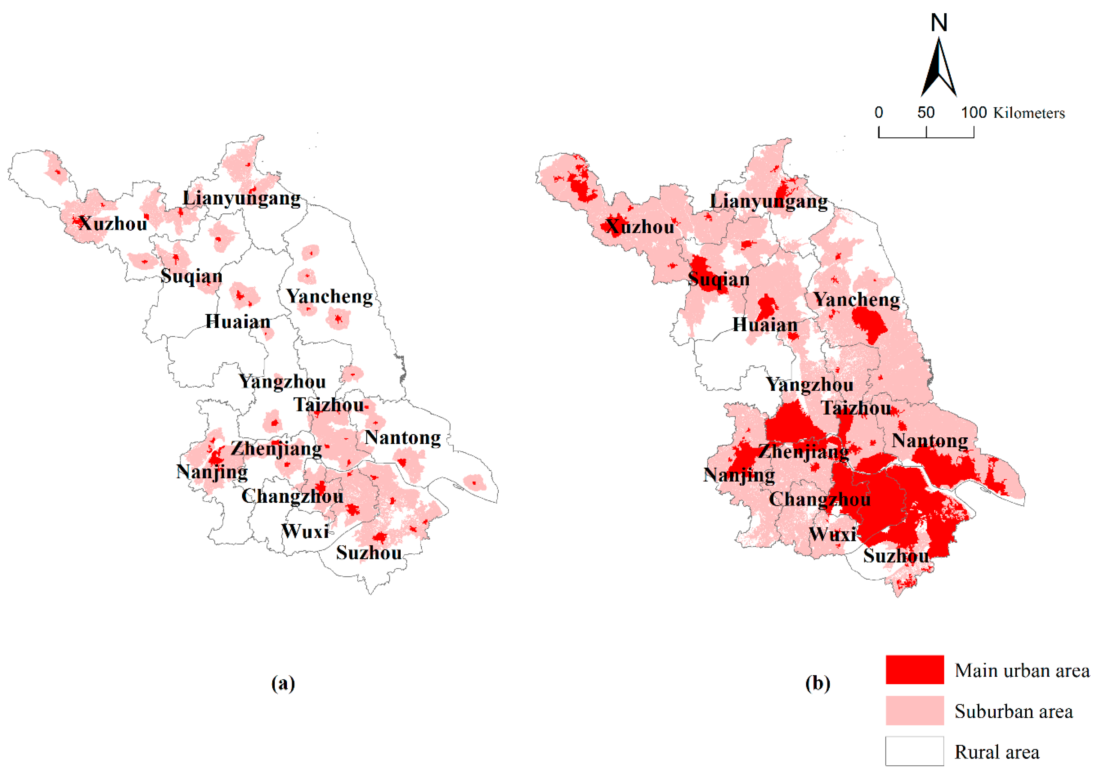
5. Results and Analyses

5.1. Mapping Suburbs Based on Spatial Interaction Estimations

To evaluate spatial interactions at a 30 m grid scale, first, the population distributions in 1998 and 2018 were estimated. For each prefecture-level city, two regression models between the population and the independent variables were developed at the county level for 1998 and 2018, respectively. The values of $R^2$ range from 0.67 to 0.81, and all values of significance are smaller than 0.1, which shows the good performance of the developed regression models (

Table 4. The summary table of the regression analysis.

City	1998		2018
	${\mathit{R}}^2$	Significance	${\mathit{R}}^2$	Significance
Changzhou	0.773	0.022	0.767	0.048
Huaian	0.754	0.082	0.75	0.049
Liangyungang	0.679	0.079	0.714	0.058
Nanjing	0.72	0.063	0.738	0.018
Nantong	0.724	0.084	0.755	0.066
Suqian	0.722	0.057	0.76	0.037
Suzhou	0.805	0.080	0.806	0.005
Taizhou	0.733	0.082	0.674	0.041
Wuxi	0.734	0.094	0.732	0.028
Xuzhou	0.766	0.053	0.79	0.014
Yancheng	0.744	0.023	0.773	0.000
Yangzhou	0.766	0.030	0.672	0.082
Zhenjiang	0.687	0.081	0.732	0.037

).

The population distributions in 1998 and 2018 were estimated. To further assess the estimation accuracy, the estimated population at a 30 m grid scale was summed to the prefectural city level and compared with the data from the statistical yearbook. Then, a linear regression analysis was conducted and the R² values were 0.82 and 0.87 in 1998 and 2018, respectively.

Then, we utilized the estimated population to quantify spatial interactions and to detect the boundaries of the suburbs. First, the main urban area was identified based on the traditional method of using population and residential land. In each prefecture-city, the population distribution was classified into high, medium, and low density using the natural break method. Then, the overlapping area of high and medium population density and the construction land was identified as the main urban area.

Then, the whole study area was divided into 30 m grids, and the grids that were located in the main area were set to “1” as the main urban area grids. For the rest of the grids, their spatial interactions with the main urban grids were calculated; if the value fell between -0.5 and 0.5, the grid was set to “2” as the suburban grid. Finally, the remaining grids were set to “3” as the rural grids. Figure 2. shows the mapped main urban, suburban, and rural areas in 1998 and 2018.

To verify the accuracy of the mapped urban, suburban, and rural areas, the classification based on the construction land density was conducted and compared.

Table 5. The overlapping area proportion to the classification results based on the construction land density.

City	1998		2018
	Urban	Suburban	Urban	Suburban
Changzhou	76.76%	65.08%	91.80%	80.47%
Huaian	84.00%	63.25%	78.30%	74.61%
Liangyungang	72.44%	56.31%	65.98%	63.70%
Nanjing	86.47%	86.18%	92.37%	86.84%
Nantong	79.70%	69.18%	96.17%	89.44%
Suqian	71.26%	67.64%	86.77%	85.96%
Suzhou	93.50%%	68.67	89.11%	80.57%
Taizhou	98.30%	81.12%	94.71%	69.87%
Wuxi	75.32%	89.68%	94.61%	85.06%
Xuzhou	75.51%	79.24%	97.49%	80.54%
Yancheng	88.49%	62.88%	83.48%	71.15%
Yangzhou	80.81%	68.67%	93.19%	75.67%
Zhenjiang	80.00%	85.49%	96.75%	91.38%

shows the overlapping area proportion to the classification results based on the construction land density.

From the table, the proportions of the overlapping area by the spatial interaction estimation and the conventional construction land density of the urban areas were generally higher than that of the suburbs. On the one hand, the identified urban areas refer to the population density and construction land distribution. Therefore, the respondent overlapping proportion is high. On the other hand, the definition of suburbs never reaches a common standard; hence, there exists vagueness in the density classification of suburbs for both population and construction land density. Nevertheless, the overlapping area proportion of the suburbs still reaches at least 62.88%, which indicates the accuracy of the mapped boundaries of suburbs. To further improve the identification accuracy, other methods such as local residents’ investigation about the conceptual definition can be added in the future.

The areas of the mapped main urban, suburban, and rural areas in 1998 were 106.96 ${\mathrm{km}}^2$ (1.37%), 1882.38 ${\mathrm{km}}^2$ (24.08%), and 5829.04 ${\mathrm{km}}^2$ (74.56%), respectively, which shifted, in 2018, to 1518.63 ${\mathrm{km}}^2$ (19.42%), 4417.89 ${\mathrm{km}}^2$ (56.51%), and 1881.86 ${\mathrm{km}}^2$ (24.07%), respectively. This shows that during the 20 years, the scope of the main urban and suburban areas of Jiangsu expanded greatly. Conversely, the rural areas shrank by 67.7%.

5.2. Land-Use Changes in Suburban Jiangsu from 1998 to 2018

Along with the urban construction land expansion, the interactions between urban and suburban areas change simultaneously, and the scope of the suburbs also changes. A land-use transfer matrix was developed to describe the land-use structure changes in the suburban expansion area (

Table 6. The land-use transfer matrix of the suburban expansion area.

Land Use Type	Cropland (2018)	Forest (2018)	Grassland (2018)	Waterbody (2018)	Construction Land (2018)	Unused (2018)
Cropland (1998)	72.34%	3.19%	0.72%	1.34%	22.41%	0.01%
Forest (1998)	26.75%	49.14%	0.66%	1.18%	22.23%	0.04%
Grassland (1998)	50.68%	22.12%	0.84%	1.06%	25.25%	0.06%
Waterbody (1998)	36.48%	2.46%	1.97%	34.00%	25.00%	0.09%
Construction land (1998)	32.34%	2.05%	0.88%	2.28%	62.42%	0.04%
Unused (1998)	25.64%	8.62%	0.47%	7.93%	57.34%	0.00%

).

Within the scope of the suburban expansion area, the land transition was drastic over the 20 years. From the table, the proportion of cropland decreased by 27.66%. However, since the original amount of cropland was huge, the decrease amount was still considerable (99.41${\mathrm{km}}^2$). The proportion of the decreased area of forest was the biggest. In addition, the decrease of grassland and waterbody was also considerable, with areas of 2.94 and 10.53 ${\mathrm{km}}^2$, respectively. The table also indicates that a lot of unused land was utilized for construction land over the 20 years. However, the total amount of unused land was small; therefore, the ecological land was the main source for the construction land development in Jiangsu from 1998 to 2018.

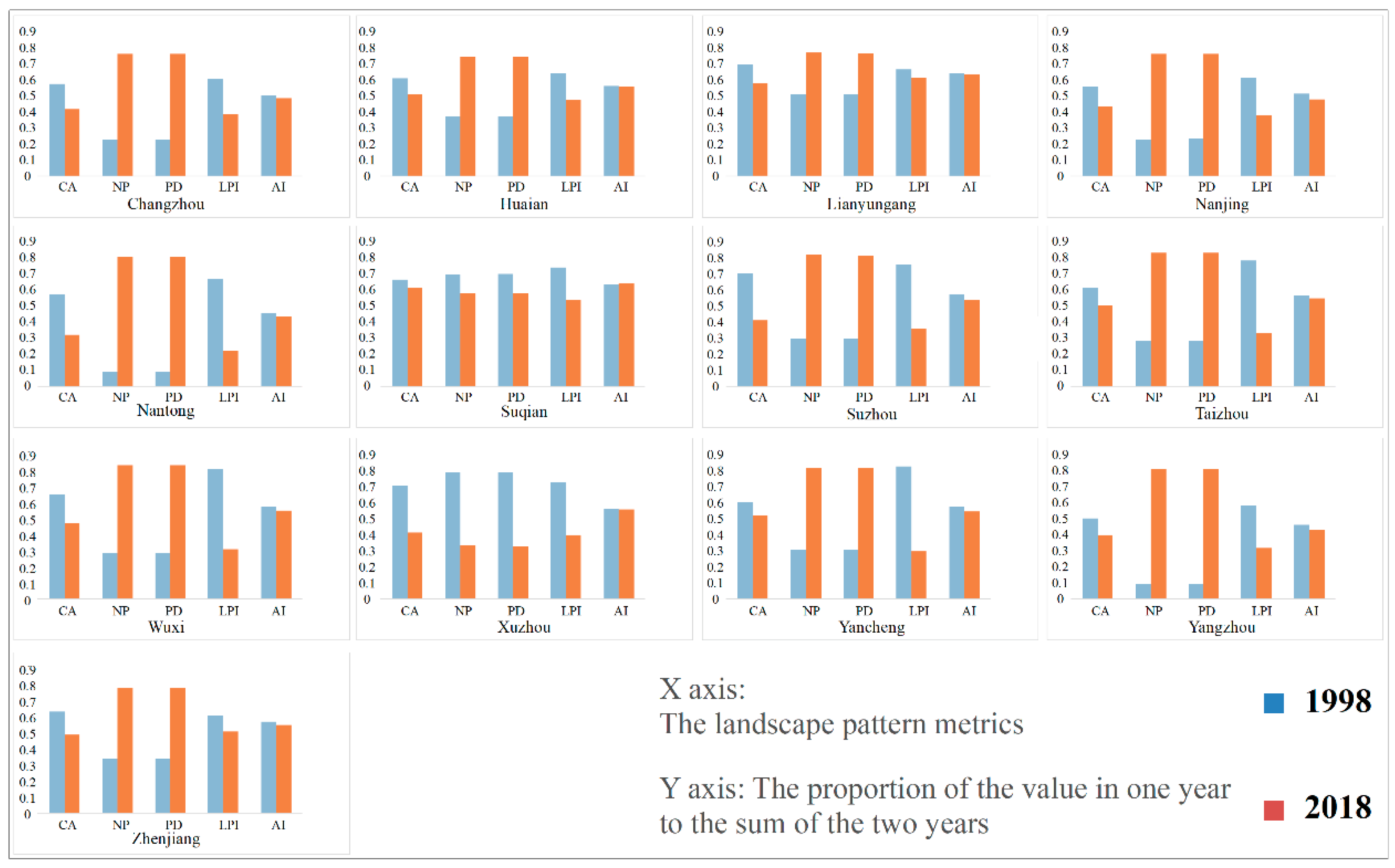
5.3. The Ecological Landscape Changes in Suburban Jiangsu

To analyze the effects of suburban expansion on ecological landscape patterns, the ecological landscape metrics of the suburban expansion area and the remaining rural area from 1998 to 2018 were calculated and compared.

At the province level,

Table 7. The ecological landscape pattern metrics at the province level from 1998 to 2018.

Landscape Pattern Index	Suburban Expansion Area		The Remained Rural Area
	1998	2018	1998	2018
CA (${\mathrm{km}}^2)$	5.00	3.93	2.39	2.32
NP	70284	153301	85383	88385
PD	1.36	2.97	3.51	3.62
LPI	45.48	12.36	28.40	29.17
AI	97.50	93.32	97.06	96.71

shows the values of the total area (CA), number of patches (NP), patch density (PD), largest patch index (LPI), and aggregation index (AI) of the suburban expansion area and the remaining rural area of Jiangsu.

As shown in Table 7, at the provincial level, the total area of ecological land decreased significantly from 1998 to 2018. At the same time, the ecological land patch number and density obviously increased. However, the largest patch index decreased from 45.48 to 12.36, which indicates that the ecological land became fragmented. In addition, the aggregation index changed from 97.5 to 93.32, showing that the distribution of ecological land became unaggregated. For comparison, the ecological landscape in the remaining rural area did not show many changes.

Figure 3 shows the ecological landscape metrics change at the prefectural city level. This figure mainly illustrates the changes of each landscape pattern metric between the two years of 1998 and 2018, and each bar is based on the proportion of one landscape pattern metric to the sum of the two years.

Figure 3 shows that the total area of ecological land in each city decreased during the 20 years. Meanwhile, except for Suqian, the ecological land patch numbers and density of all other cities clearly increased, indicating that the ecological land became scattered. The decrease in the LPI corresponds with the finding that the ecological landscape underwent fragmentation over time. In addition, considering the supporting and provisioning services offered by ecological land, the decrease in LPI also reveals the threat of suburban expansion to ecological function and biodiversity. The values of the AI of all cities experienced a loss over time. However, the change in AI was slight in some cities, such as Huaian, Suqian, and Xuzhou because the number and density of the ecological land patches increased, which affected the aggregation of ecological land at the collective level. Taken together, the decrease in the total area, largest patch area, and aggregation level and the increases in the patch numbers and density demonstrate the shrinkage and division of the ecological land in suburban expansion areas.

For comparison, the ecological landscape metrics of the remaining rural areas in each prefecture-level city were also calculated. Similar to the results at a provincial level, the ecological landscape in the rural area showed little change.

Table 8. Statistical characteristics of ecological landscape metrics in the suburban expansion area and remaining rural areas (unit, ${\mathrm{m}}^2$).

Value	Minimum		Maximum		Average
Area	Suburb	Rural	Suburb	Rural	Suburb	Rural
CA	−289,676.79	−21,155.8	−28,543.23	59.85	−82,441.72	−5427.46
NP	−2942.00	−314	17,228.00	898	6402.08	222.00
PD	−0.46	−0.63	4.44	0.49	1.91	0.12
LPI	−64.47	−25.23	−3.95	12.27	−27.12	−4.36
AI	−5.76	−1.44	0.71	0.16	−2.50	−0.53

displays the minimum, maximum, and average standard deviation values of the suburban expansion area and the remaining rural area after calculating the change values of the five selected landscape pattern metrics at the prefectural city level.

On the basis of the comparison results, the ecological landscape changed drastically in the suburban expansion area as compared with rural areas. The results also indicate that there is obvious spatial heterogeneity in the ecological landscape changes in different prefecture-levl cities. Specifically, Nantong, Yancheng, Suzhou, and Yangzhou experienced the largest ecological land decrease (more than 90,000 ${\mathrm{m}}^2$), while Nanjing, Taizhou, Wuxi, and Yancheng experienced the most severe ecological land fragmentation, showing a sharp decrease in the largest patch index. Nantong, Changzhou, Yancheng, and Yangzhou had the largest AI decrease, indicating the unaggregated distribution trend of the ecological land in their suburban expansion areas. Yancheng had the largest decrease in the ecological land area, as well as the largest patch index and aggregation index, showing the seriousness of ecological landscape degradation in the region.

Conversely, there was little change in the ecological landscape metrics in the remaining rural areas. Specifically, the standard deviation values of PD, LPI, and AI were small, indicating that the change was slight. On the basis of the comparison of the ecological landscape changes in the suburban expansion area and the remaining rural area, it was concluded that suburban expansion contributes much to ecological landscape degradation, while the rural area produces little effect.

6. Discussion

6.1. Spatial Interaction and Suburban Change

For many years, land change analyses were affected deeply by the “urban-rural” dichotomy, wherein urban centers and suburbs were treated as one and the same [48]. Therefore, there are many studies on urban land expansion and its social, economic, and ecological effects. By realizing the differences between the main urban, suburban, and rural areas, efforts have been made in identifying and analyzing the dynamic evolution of urban spatial structures. Despite the differences in population and residential land density between urban, suburban, and urban areas, spatial interaction is another important indicator that can differentiate urban spatial structures.

At the urban center, the density of the population and construction land is at a high level. Usually, the city center is also a place where multiple urban functions are concentrated. The central place theory proposes that the population that a central area serve is determined by the number of kinds of services that it can offer [49,50]. Because of the many services of the urban center, people that inhabit other areas are attracted to visit the urban center to conduct activities, ranging from daily activities such as working to non-daily activities such as attending an exhibition [51]. In this way, the flows of people, material, and information are formed spatially. From this perspective, the spatial interactions inside the main urban area are the most active. On the one hand, the population density is the highest in the main urban area, and spatial interactions are driven by people’s daily life demands, which is the endogenous reason for spatial interactions. On the other hand, varied city services help satisfy peoples’ demands, which is the external cause of these interactions. In the suburbs, although the density of the population and residential land is lower than that of the main urban area, and its land-use function is also simpler, urban and suburban areas experience close interactions. For example, in developing countries such as China, the land use of suburbs is dominated by factories and residential land due to close proximity of suburbs to the urban center and the low price of settlement [52,53]. There are close suburban-urban relationships, such as the provision of materials and interactions of commuting. The attraction of urban services and spatial accessibility enables the occurrence of suburban–urban interaction. In rural areas, the population and residential land are distributed sparsely. Moreover, the land-use function here is the simplest compared to other urban structures. Therefore, the interactions between rural and non-rural areas is weak. There are also spatial interaction differences in urban, suburban, and rural areas in developed areas. For example, the commuting relationship between urban and suburbs is obvious in developed cities such as Amsterdam, Tokyo, and New York [54,55,56]. However, such interactions are usually studied as one characteristic of the suburbs, and insufficiently referenced to map the boundaries of suburbs. Due to the heterogeneity of spatial interactions, the main urban, suburban, and rural areas can be identified, which is possible in both developing and developed cities.

This study mainly utilized the population distribution to estimate the spatial interaction. Other methods that can evaluate the spatial relationship can also be applied. For example, the gravity model, which is widely applied to quantify city connection, can be referenced based on population and economic data to simulate the spatial interaction. In addition, transportation flow based on the road network, social connection based on SNS data, and economic flow based on chain-industry can be also integrated to elaborate the spatial interaction evaluation. Especially in developed countries, where urban expansion can be insignificant, relationships, such as commuting between urban and suburban areas, can be used to distinguish the urban, suburban, and rural areas from each other.

6.2. The Effects of Suburban Expansion on the Ecological Landscape

The negative effects of urban expansion have been analyzed sufficiently in existing studies. Usually, the boundary of the continuous urban construction land is mapped utilizing remote sensing data. It has been demonstrated that the biggest source of urban land is ecological land. Moreover, the relationships among urban expansion and ecosystem function, service, and landscape has been explored [11,57,58]. However, the emphasis on urban expansion in the literature neglects the impacts of suburban expansion. The effects of suburban expansion on the ecological environment can be classified as direct and implicit effects. First, suburbs are composed of urban and rural areas. The spatial scope of suburbs covers part of the urban construction land and part of the non-urban land. Under the background of rapid urbanization, the edge of the urban construction land expands rapidly, and thus exerts direct pressure on the ecological environment. From the perspective of land-use change, large-scale non-urban land, including cropland, forest, and grassland, transitions into urban land, and the total area of ecological land decreases. Second, implicit pressure comes from the frequent spatial interactions between urban and suburban areas. Due to the spatial proximity and low price of land rent, many factories are aggregately distributed in the suburbs. For example, in China, newly-built industrial parks tend to be built in the suburbs [59]. Furthermore, to solve the conflict between high-living costs and occupational opportunities in the urban center, some people settle in the suburbs, which drives residential land construction in the suburbs. In addition, material transportation and people’s daily commuting activities generate demands for public infrastructure development (such as road networks), which also increases the chance of a land transition in the suburbs. The resources consumed and pollutants released due to production and living activities during such interactions create potential ecological risks.

By comparing the ecological landscape patterns in the suburban expansion area and the remaining rural area, this study verified the negative effects of suburban expansion on ecological land decrease and landscape fragmentation. From 1998 to 2018, the ecological land in the suburban expansion area of Jiangsu Province decreased sharply from 5 to 3.93 ${\mathrm{km}}^2$; meanwhile, the ecological land area in the remaining rural area only decreased by 0.07 ${\mathrm{km}}^2$. At the prefectural city level, the ecological land area of all 13 cities decreased. In addition, the increase in the ecological land patch and density also indicates that the distribution of ecological land in suburban Jiangsu became fragmented. Moreover, the aggregation level of the ecological land showed a decreasing trend, which agrees with the fragmentation trend of the ecological land. For comparison, the ecological landscape in the remaining rural area at the prefectural city level did not show significant changes over the 20 years. Existing studies have demonstrated the effects of urban construction land expansion. This study focused on the sprawl of suburbs and proved that the impacts of suburban expansion on the ecological landscape should not be neglected.

By studying the ecological landscape of suburban Jiangsu, this study also found that Yancheng, which is one of the 13 prefecture-level cities of Jiangsu, experienced the largest decrease in ecological land area, ecological land patch area, and aggregation level, thereby revealing a drastic ecological risk due to the suburban expansion. Ecological land protection, aggregation, and construction should be considered in the future city development and management of Yancheng.

6.3. The Implications of Suburban Identification on Suburban and Ecological Landscape Planning

The identification of suburbs has practical significance for suburban and ecological landscape planning. The implementation of suburban planning is usually based on factors such as urban-rural function integration, ecological protection, and industrial complementation. For example, the construction land scale in suburbs is generally determined based on the population growth in the future of the city. In addition, the allocation of construction land in suburbs is also restricted to protected areas such as the primary land, ecological preservation land, and traditional towns. The control and governance from the local government to balance the social, economic, ecological, and cultural benefits affect the form and development of suburbs. Mapping the boundaries of suburbs, therefore, is helpful to assess the suburban development in the past, and to find the potential conflict area in the future. On the one hand, the mapping boundaries are developed based on population distribution and spatial interaction estimation. By comparing the current boundaries with the suburban planning set in the past, assessment on the land-use efficiency, ecological protection, and traditional town preservation can be made. On the other hand, by simulating the population increase and spatial interaction in the future, the suburban growth can be simulated. By checking the overlapping areas of suburbs, especially construction land, with the protected areas, conflict areas can be identified, and special protection strategies can be made.

For ecological landscape planning, suburban identification can offer decision support for ecological security assessments and ecosystem service function assessments. Ecological security is defined as “mankind’s degree of assurance unaffected by ecological destruction and environmental pollution in yield, living, and health” [60]. An ecological security assessment can be used to evaluate ecological carrying capacity, urban development potential, and regional development sustainability, and it is an important factor of ecological protection. The “pressure-status-response” (PSR) model is one of the most commonly applied methods for conducting an ecological security assessment. The “stress” indicator refers specifically to the results of gathering natural resources and generating pollutants due to human needs for various social and economic activities, thereby exerting pressure on the ecological environment. “Status” refers to the state of the environment facing the pressure of such human activities, and “response” denotes human corresponding actions to solve such ecological problems. This study verified that the ecological landscape tends to be more fragmented in the suburbs than in rural areas. Therefore, the identification of suburbs can be utilized as an indicator of the “pressure” exerted by explicit and implicit human impacts.

Ecosystem service function refers to the ability of the ecological environment to maintain various human activities. It includes ecological functions such as food supply, soil and water conservation, wind and sand fixation, and flood storage and also cultural services. The landscape pattern is one of the essential factors that affect the ecosystem service function, including land area and morphological changes. By mapping the boundaries of suburbs, the ecosystem service value can be evaluated and traced, allowing protection planning to be developed and adjusted. In some developed countries, to protect natural scenic rural areas and traditional towns, strategies like delineating “green belt” zones are used to protect rural areas from urban expansion [61,62]. In developing countries, it is important to balance land demands for urbanization and land reservations for ecological protection. On the basis of the analysis results of this study, the ecosystem service function of a city changes greatly during suburban expansion. Hence, strategies such as the “green belt” policy can be applied within suburban expansion to protect important ecological areas.

6.4. Priorities in Future Studies

There are several limitations to this study that can be prioritized in future studies. First, the regression model for estimating population distribution is simple. To increase the estimation accuracy, high-resolution remote sensing images could be referenced in the future, and more factors could be integrated. Second, this study evaluates spatial interactions based on people flow simulated by the radiation model. However, the interactions between urban and suburbs are complicated. More indicators such as traffic flow, mobile phone data, and people’s daily activity diaries could be referenced in the future to elaborate on such spatial interactions. Third, more methods could be applied to map the boundaries of suburbs, such as using a questionnaire investigation to analyze the conceptual recognition of local residents, thereby increasing the accuracy of mapping the boundaries of suburbs.

7. Conclusions

This study identifies the boundaries of suburbs by considering their spatial interactions at a 30 m grid level. This study analyzes the effects of suburban expansion on ecological landscape pattern changes based on mapping the main urban, suburban, and rural areas of Jiangsu Province, in 1998 and 2018. The results demonstrate that suburban expansion was evident over the past 20 years. In addition, by comparing the ecological landscape pattern changes in the suburban expansion area and the remaining rural area, it was concluded that the ecological land in the suburban expansion area decreased significantly and that its distribution showed a trend of fragmentation at both the province level and the prefectural city level. Concerning the significant effects of suburban expansion on the ecological landscape, this study provides two examples of integrating suburban identification into ecological planning, including ecological security assessment and ecosystem service function evaluation.

This study contributes to understanding suburbs from the perspective of spatial interaction, thereby enriching the theoretical framework of suburban studies and verifying the effects of suburban expansion on ecological landscape patterns.

References

1. Gu, C.; Guan, W.; Liu, H. Chinese urbanization 2050: SD modeling and process simulation. Sci. China Earth Sci. 2017, 60, 1067–1082. [Google Scholar] [CrossRef]
2. D’Amour, C.B.; Reitsma, F.; Baiocchi, G.; Barthel, S.; Güneralp, B.; Erb, K.-H.; Haberl, H.; Creutzig, F.; Seto, K.C. Future urban land expansion and implications for global croplands. Proc. Natl. Acad. Sci. USA 2017, 114, 8939–8944. [Google Scholar] [CrossRef] [PubMed] [Green Version]
3. Fazal, S. Urban expansion and loss of agricultural land-a GIS based study of Saharanpur City, India. Environ. Urban. 2000, 12, 133–149. [Google Scholar] [CrossRef]
4. Peng, J.; Pan, Y.; Liu, Y.; Zhao, H.; Wang, Y. Linking ecological degradation risk to identify ecological security patterns in a rapidly urbanizing landscape. Habitat Int. 2018, 71, 110–124. [Google Scholar] [CrossRef]
5. Long, H.; Liu, Y.; Hou, X.; Li, T.; Li, Y. Effects of land use transitions due to rapid urbanization on ecosystem services: Implications for urban planning in the new developing area of China. Habitat Int. 2014, 44, 536–544. [Google Scholar] [CrossRef]
6. Nuissl, H.; Haase, D.; Lanzendorf, M.; Wittmer, H. Environmental impact assessment of urban land use transitions—A context-sensitive approach. Land Use Policy 2009, 26, 414–424. [Google Scholar] [CrossRef]
7. Salvati, L. Monitoring high-quality soil consumption driven by urban pressure in a growing city (Rome, Italy). Cities 2013, 31, 349–356. [Google Scholar] [CrossRef]
8. Zhao, Y.; Wang, Z.; Sun, W.; Huang, B.; Shi, X.; Ji, J. Spatial interrelations and multi-scale sources of soil heavy metal variability in a typical urban–rural transition area in Yangtze River Delta region of China. Geoderma 2010, 156, 216–227. [Google Scholar] [CrossRef]
9. Yin, J.; Yin, Z.; Zhong, H.; Xu, S.; Hu, X.; Wang, J.; Wu, J. Monitoring urban expansion and land use/land cover changes of Shanghai metropolitan area during the transitional economy (1979–2009) in China. Environ. Monit. Assess. 2011, 177, 609–621. [Google Scholar] [CrossRef]
10. Batisani, N.; Yarnal, B. Urban expansion in Centre County, Pennsylvania: Spatial dynamics and landscape transformations. Appl. Geogr. 2009, 29, 235–249. [Google Scholar] [CrossRef]
11. Zank, B.; Bagstad, K.J.; Voigt, B.; Villa, F. Modeling the effects of urban expansion on natural capital stocks and ecosystem service flows: A case study in the Puget Sound, Washington, USA. Landsc. Urban. Plan. 2016, 149, 31–42. [Google Scholar] [CrossRef]
12. Kukkonen, M.O.; Muhammad, M.J.; Käyhkö, N.; Luoto, M. Urban expansion in Zanzibar City, Tanzania: Analyzing quantity, spatial patterns and effects of alternative planning approaches. Land Use Policy 2018, 71, 554–565. [Google Scholar] [CrossRef]
13. Forsyth, A. Defining suburbs. J. Plan. Lit. 2012, 27, 270–281. [Google Scholar] [CrossRef] [Green Version]
14. Lang, R.E.; Blakely, E.J.; Gough, M.Z. Keys to the new metropolis: America’s big, fast-growing suburban counties. J. Am. Plan. Assoc. 2005, 71, 381–391. [Google Scholar] [CrossRef]
15. Vaughan, L.; Griffiths, S.; Haklay, M.; Jones, C.E. Do the suburbs exist? Discovering complexity and specificity in suburban built form. Trans. Inst. Br. Geogr. 2009, 34, 475–488. [Google Scholar] [CrossRef] [Green Version]
16. Harris, R.; Larkham, P. Changing Suburbs: Foundation, Form and Function; Routledge: Abingdon-on-Thames, UK, 2003. [Google Scholar]
17. Mace, A. Suburbanization; Elsevier: Amsterdam, The Netherlands, 2009. [Google Scholar]
18. Clapson, M.; Hutchison, R. Introduction: Suburbanization in global society. Res. Urban. Sociol. Suburb. Glob. Soc. 2010, 10, 1–14. [Google Scholar]
19. Liu, Y.; Diao, Q.; Kou, M.; Tian, Z.; Leng, B. Primary Study on Land Use of Suburb Landscape BAsed on TM Images——A Case Study in Shahe, Changping Distirct, Beijing. Remote Sens. Technol. Appl. 2011, 20, 563–568. [Google Scholar]
20. Rudel, T.K. How do people transform landscapes? A sociological perspective on suburban sprawl and tropical deforestation. Am. J. Sociol. 2009, 115, 129–154. [Google Scholar] [CrossRef]
21. Jay, J.E. The Malling of Vermont: Can the Growth Center Designation Save the Traditional Village from Suburban Sprawl. Vt. L. Rev. 1996, 21, 929. [Google Scholar]
22. Fuller, R.A.; Irvine, K.N. Interactions between people. Urban. Ecol. 2010, 134. [Google Scholar] [CrossRef]
23. Zeng, C.; Liu, Y.; Stein, A.; Jiao, L. Characterization and spatial modeling of urban sprawl in the Wuhan Metropolitan Area, China. Int. J. Appl. Earth Obs. Geoinf. 2015, 34, 10–24. [Google Scholar] [CrossRef]
24. Forman, R.T. Urban. Regions: Ecology and Planning beyond the City; Cambridge University Press: Cambridge, UK, 2008. [Google Scholar]
25. Banzhaf, E.; Reyes-Paecke, S.; Müller, A.; Kindler, A. Do demographic and land-use changes contrast urban and suburban dynamics? A sophisticated reflection on Santiago de Chile. Habitat Int. 2013, 39, 179–191. [Google Scholar] [CrossRef]
26. Johnson, L.; Andrews, F.; Warner, E. The centrality of the Australian suburb: Mobility challenges and responses by outer suburban residents in Melbourne. Urban. Policy Res. 2017, 35, 409–423. [Google Scholar] [CrossRef]
27. Gordon, D.L.; Janzen, M. Suburban nation? Estimating the size of Canada’s suburban population. J. Archit. Plan. Res. 2013, 197–220. [Google Scholar]
28. Heris, M.P. Evaluating metropolitan spatial development: A method for identifying settlement types and depicting growth patterns. Reg. Stud. Reg. Sci. 2017, 4, 7–25. [Google Scholar] [CrossRef] [Green Version]
29. Gober, P.; Behr, M. Central cities and suburbs as distinct place types: Myth or fact? Econ. Geogr. 1982, 58, 371–385. [Google Scholar] [CrossRef]
30. Paccoud, A.; Mace, A. Tenure change in London’s suburbs: Spreading gentrification or suburban upscaling? Urban. Stud. 2018, 55, 1313–1328. [Google Scholar] [CrossRef] [Green Version]
31. Gianotti, A.G.S.; Getson, J.M.; Hutyra, L.R.; Kittredge, D.B. Defining urban, suburban, and rural: A method to link perceptual definitions with geospatial measures of urbanization in central and eastern Massachusetts. Urban. Ecosyst. 2016, 19, 823–833. [Google Scholar] [CrossRef]
32. Nechyba, T.J.; Walsh, R.P. Urban sprawl. J. Econ. Perspect. 2004, 18, 177–200. [Google Scholar] [CrossRef] [Green Version]
33. Oueslati, W.; Alvanides, S.; Garrod, G. Determinants of urban sprawl in European cities. Urban. Stud. 2015, 52, 1594–1614. [Google Scholar] [CrossRef] [Green Version]
34. Yue, W.; Liu, Y.; Fan, P. Measuring urban sprawl and its drivers in large Chinese cities: The case of Hangzhou. Land Use Policy 2013, 31, 358–370. [Google Scholar] [CrossRef]
35. Novak, A.B.; Wang, Y. Effects of suburban sprawl on Rhode Island’s forests: A landsat view from 1972 to 1999. Northeast. Nat. 2004, 11, 67–74. [Google Scholar] [CrossRef]
36. Radeloff, V.C.; Hammer, R.B.; Stewart, S.I. Rural and suburban sprawl in the US Midwest from 1940 to 2000 and its relation to forest fragmentation. Conserv. Biol. 2005, 19, 793–805. [Google Scholar] [CrossRef]
37. Liang, C.; Penghui, J.; Manchun, L.; Liyan, W.; Yuan, G.; Yuzhe, P.; Nan, X.; Yuewei, D.; Qiuhao, H. Farmland protection policies and rapid urbanization in China: A case study for Changzhou City. Land Use Policy 2015, 48, 552–566. [Google Scholar] [CrossRef]
38. Wang, H.; Shi, Y.; Zhang, A.; Cao, Y.; Liu, H. Does Suburbanization Cause Ecological Deterioration? An Empirical Analysis of Shanghai, China. Sustainability 2017, 9, 124. [Google Scholar] [CrossRef] [Green Version]
39. Kahn, M.E. The environmental impact of suburbanization. J. Policy Anal. Manag. 2000, 19, 569–586. [Google Scholar] [CrossRef]
40. Holian, M.J.; Sridhar, K.S. The role of road infrastructure and air pollution in the recent suburbanization of India’s cities: An exploration. Environ. Urban. Asia 2017, 8, 151–169. [Google Scholar] [CrossRef]
41. Kim, H.W.; Li, M.-H.; Kim, J.-H.; Jaber, F. Examining the impact of suburbanization on surface runoff using the SWAT. Int. J. Environ. Res. 2016, 10, 379–390. [Google Scholar]
42. Peng, J.; Zhao, M.; Guo, X.; Pan, Y.; Liu, Y. Spatial-temporal dynamics and associated driving forces of urban ecological land: A case study in Shenzhen City, China. Habitat Int. 2017, 60, 81–90. [Google Scholar] [CrossRef]
43. Maes, J.; Liquete, C.; Teller, A.; Erhard, M.; Paracchini, M.L.; Barredo, J.I.; Grizzetti, B.; Cardoso, A.; Somma, F.; Petersen, J.-E. An indicator framework for assessing ecosystem services in support of the EU Biodiversity Strategy to 2020. Ecosyst. Serv. 2016, 17, 14–23. [Google Scholar] [CrossRef] [Green Version]
44. Wang, J.; He, T.; Lin, Y. Changes in ecological, agricultural, and urban land space in 1984–2012 in China: Land policies and regional social-economical drivers. Habitat Int. 2018, 71, 1–13. [Google Scholar] [CrossRef]
45. Chen, Q.; Hou, X.; Wu, L. Comparing of population spatialization models based on land use data and DMSP/OLS data respectively: A case study in the efficient ecological economic zone of the Yellow River Delta. Hum. Geogr. 2014, 29, 94–100. [Google Scholar]
46. Simini, F.; González, M.C.; Maritan, A.; Barabási, A.-L. A universal model for mobility and migration patterns. Nature 2012, 484, 96–100. [Google Scholar] [CrossRef] [PubMed]
47. Tian, Y.; Kong, X.; Liu, Y.; Wang, H. Restructuring rural settlements based on an analysis of inter-village social connections: A case in Hubei Province, Central China. Habitat Int. 2016, 57, 121–131. [Google Scholar] [CrossRef]
48. Serra, P.; Vera, A.; Tulla, A.F.; Salvati, L. Beyond urban–rural dichotomy: Exploring socioeconomic and land-use processes of change in Spain (1991–2011). Appl. Geogr. 2014, 55, 71–81. [Google Scholar] [CrossRef]
49. Smith, M.W. A guide to the delineation of medical care regions, medical trade areas, and hospital service areas. Public Health Rep. 1979, 94, 248. [Google Scholar]
50. Smith, M. The economics of physician location. In Proceedings of Western Regional Conference; American Association of Geographers: Chicago, IL, USA, 1979. [Google Scholar]
51. Tian, Y.; Kong, X.; Liu, Y. Combining weighted daily life circles and land suitability for rural settlement reconstruction. Habitat Int. 2018, 76, 1–9. [Google Scholar] [CrossRef]
52. Liu, Y.; Yue, W.; Fan, P.; Peng, Y.; Zhang, Z. Financing China’s suburbanization: Capital accumulation through suburban land development in Hangzhou. Int. J. Urban. Reg. Res. 2016, 40, 1112–1133. [Google Scholar] [CrossRef]
53. Xiao, J.; Shen, Y.; Ge, J.; Tateishi, R.; Tang, C.; Liang, Y.; Huang, Z. Evaluating urban expansion and land use change in Shijiazhuang, China, by using GIS and remote sensing. Landsc. Urban. Plan. 2006, 75, 69–80. [Google Scholar] [CrossRef]
54. Mattingly, P.H. Suburban Landscapes: Culture and Politics in a New York Metropolitan Community; JHU Press: Baltimore, MD, USA, 2001. [Google Scholar]
55. Ohashi, H. Suburban Fortunes: Urban Policies, Planning and Suburban Transformation in Tokyo Metropolis; UCL (University College London): London, UK, 2018. [Google Scholar]
56. Tzaninis, Y.; Boterman, W. Beyond the urban–suburban dichotomy: Shifting mobilities and the transformation of suburbia. City 2018, 22, 43–62. [Google Scholar] [CrossRef]
57. Nor, A.N.M.; Corstanje, R.; Harris, J.A.; Brewer, T. Impact of rapid urban expansion on green space structure. Ecol. Indic. 2017, 81, 274–284. [Google Scholar] [CrossRef]
58. Xie, W.; Huang, Q.; He, C.; Zhao, X. Projecting the impacts of urban expansion on simultaneous losses of ecosystem services: A case study in Beijing, China. Ecol. Indic. 2018, 84, 183–193. [Google Scholar] [CrossRef]
59. Zhu, F.; Zhang, F.; Ke, X. Rural industrial restructuring in China’s metropolitan suburbs: Evidence from the land use transition of rural enterprises in suburban Beijing. Land Use Policy 2018, 74, 121–129. [Google Scholar] [CrossRef]
60. Xiao, D.; Chen, W. On the basic concepts and contents of ecological security. Ying Yong Sheng Tai Xue Bao = J. Appl. Ecol. 2002, 13, 354–358. [Google Scholar]
61. Hanley, N.; Knight, J. Valuing the environment: Recent UK experience and an application to green belt land. J. Environ. Plan. Manag. 1992, 35, 145–160. [Google Scholar] [CrossRef]
62. Amati, M. Green belts: A twentieth-century planning experiment. In Urban Green Belts in the Twenty-First Century; Routledge: Abingdon-on-Thames, UK, 2016; pp. 21–38. [Google Scholar]
Figure 1. The location of Jiangsu in China and the land use of Jiangsu in 1998 (a) and in 2018 (b).
Land 09 00159 g001
Figure 2. The mapped main urban, suburban, and rural areas in 1998 (a) and 2018 (b).
Land 09 00159 g002
Figure 3. The ecological landscape metrics of each prefecture-level city of Jiangsu in 1998 (blue bar) and 2018 (red bar).
Land 09 00159 g003