Article

Nationwide Susceptibility Mapping of Landslides in Kenya Using the Fuzzy Analytic Hierarchy Process Model

1
National Center for International Research Collaboration in Building Safety and Environment, Hunan University, Changsha 410082, China
2
College of Civil Engineering, Hunan University, Changsha 410082, China
*
Author to whom correspondence should be addressed.
Land 2020, 9(12), 535; https://doi.org/10.3390/land9120535
Submission received: 18 November 2020 / Revised: 18 December 2020 / Accepted: 18 December 2020 / Published: 21 December 2020
(This article belongs to the Special Issue Landslide Hazard and Environment Risk Assessment)

Abstract

:
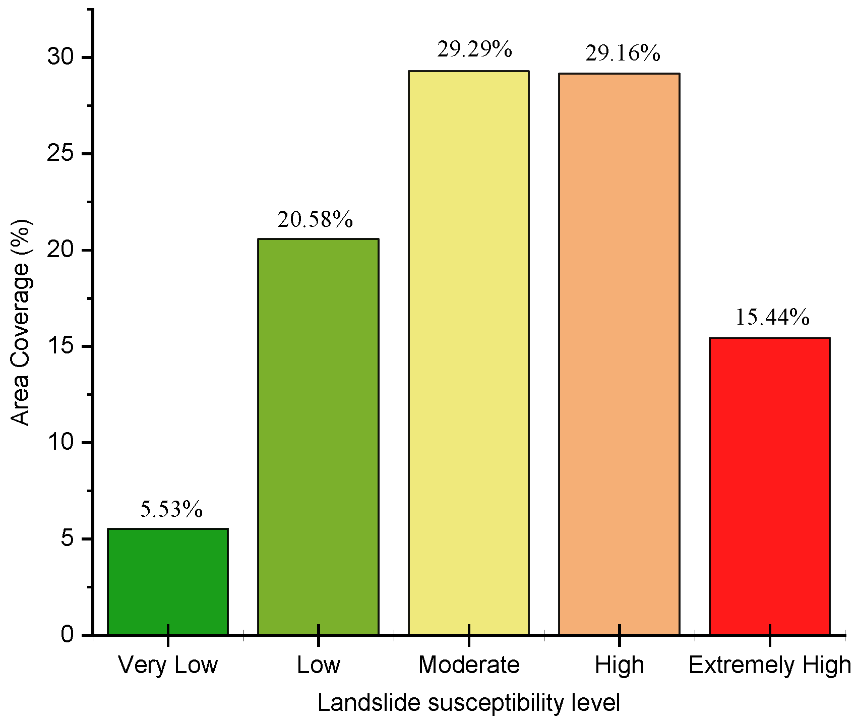
Landslide susceptibility mapping (LSM) is a cost-effective tool for landslide hazard mitigation. To date, no nationwide landslide susceptibility maps have been produced for the entire Kenyan territory. Hence, this work aimed to develop a landslide susceptibility map at the national level in Kenya using the fuzzy analytic hierarchy process method. First, a hierarchical evaluation index system containing 10 landslide contributing factors and their subclasses was established to produce a susceptibility map. Then, the weights of these indexes were determined through pairwise comparisons, in which triangular fuzzy numbers (TFNs) were employed to scale the relative importance based on the opinions of experts. Ultimately, these weights were merged in a hierarchical order to obtain the final landslide susceptibility map. The entire Kenyan territory was divided into five susceptibility levels. Areas with very low susceptibility covered 5.53% of the Kenyan territory, areas with low susceptibility covered 20.58%, areas with the moderate susceptibility covered 29.29%, areas with high susceptibility covered 29.16%, and areas with extremely high susceptibility covered 15.44% of Kenya. The resulting map was validated using an inventory of 425 historical landslides in Kenya. The results indicated that the TFN-AHP model showed a significantly improved performance (AUC = 0.86) compared with the conventional AHP (AUC = 0.72) in LSM for the study area. In total, 31.53% and 29.88% of known landslides occurred within the “extremely high” and “high” susceptibility zones, respectively. Only 8.24% and 1.65% of known landslides fell within the “low” and “very low” susceptibility zones, respectively. The map obtained as a result of this study is beneficial to inform planning and land resource management in Kenya.

1. Introduction

Every year, landslides cause a large number of deaths and enormous property losses in mountainous areas [1]. Landslides are a prehistoric issue. It is currently receiving considerable attention since damage induced by landslides has risen in recent years. Estimated fatalities from landslides reached 32,322 between 2004 and 2010, though this value is likely underestimated [2]. The situation varies in different countries. Landslides are concentrated in developing countries or regions, such as the Himalayan region and its surrounding areas in China and African countries. Hence, more effort is required to reduce landslide risks within those countries. Within this topic, the preemptive identification of landslide-prone areas through landslide susceptibility mapping (LSM) is a very promising hazard mitigation approach.
The term landslide susceptibility is a quantitative measure of the likelihood of slope failures under a particular geological condition [3]. With the increasing availability of geospatial data and rapid developments in computational science, numerous LSM methods have been proposed in the last three decades. Most of these methods were built on geographic information systems (GISs). In a broad sense, these LSM models can be summarized as qualitative (knowledge-based or inventory-based) and quantitative (statistically or physically based). In qualitative LSM modeling, each landslide factor is weighted based on the knowledge of experts in geotechnical or geological fields. Afterward, the derived weights were combined to calculate the landslide susceptibility index (LSI). Typical qualitative LSM models include heuristic analysis, inventory analysis, and analytic hierarchy processing (AHP) [4]. As a comparison, statistical LSM models quantify the weights of each factor based on the spatial correlations of historical landslides and these factors. Building on the basic assumption that “the past predicts the future”, the weights determined using historical landslides are used to predict the likelihood of future landslide occurring. Frequency ratios [5], logistic regressions [6], weights of evidence [7], artificial neural networks [8], and support vector machines [9] are frequently used statistically based LSMs in the literature. For physically based LSM models, slope stability models and groundwater flow models are integrated to calculate the safety factor for each slope unit. Several programs have been developed for LSM, such as SHALSTAB, SINMAP, and TRIGRS [10,11]. The advantages and disadvantages of different LSM models have been reviewed by Van Western et al. [12] and Reichenbach et al. [13]. Comparative studies have shown that the optimized selection of LSM methods largely depends on the scale, nature, and data availability of the study area [14,15,16].
Similar to most African countries, landslide is ranked as the deadliest geohazard in Kenya [17,18]. Despite enormous damage induced by landslides, literature reviews indicate that very few attempts have been carried out to research landslides in Kenya. The studies of landslides performed in Kenya in the past few decades have concentrated on landslide inventory mapping [19], geological investigation of single landslide events and developing general overviews of landside phenomena [18]. It is noted in the literature that intensive precipitation is a dominant factor triggering landslides in Kenya [20]. Steep topography, weathered regolith, and human activities such as deforestation, overgrazing, and overfarming have been identified as causative factors of landslides in Kenya [18]. In recent years, the continuously growing population and expansive development of infrastructure have placed a heavy burden on the environment and land resources in Kenya. No systematic research on landslide susceptibility assessment in Kenya has been published yet. Filling this research gap is the reason why this study was performed.
Difficulties remain in developing LSM for the whole territory of a country because of inadequate availability of landslide inventories and related information. As illustrated in Table 1, a literature review of some such examples showed that qualitative methods, such as spatial multicriteria evaluation (SMCE) and heuristic weighting, are the most popular existing LSM on a national scale. Van Western et al. [10] suggested that the most suitable methods for LSM at a medium scale are quantitative methods, while qualitative methods are more appropriate for LSM of large areas (small scale) [19]. The cell size of LSMs varies from coarse (1000 m) to medium (30 m) for qualitative and quantitative LSMs. The suitability of cell size is typically determined by data availability and the mapping scale [20].
The main objective of this work was to develop a landslide susceptibility map for Kenya. To conduct this, the fuzzy analytic hierarchy process (FAHP) method was adopted. This FAHP is a semiqualitative method suitable for LSM on a national scale. The landslide inventory and landslide causative factors used in this study were collected from a variety of sources. Regions highly susceptible to landslides in Kenya were highlighted as a basis for further studies of landslide hazards or risk assessments. Additionally, the output presented serves as an effective tool for the authorities involved in land planning and land resource management.

2. Study Area

Kenya is an east African country (Figure 1). Kenya has a territorial area of 582,646 km2 and a population of 41.8 million. The elevation of Kenya stretches from sea level in the coastal regions to over 5000 m above sea level (a.s.l.) at Mount Kenya. Geomorphologically, the landforms in Kenya are dominated by highlands in the central and the west regions, plains in the northeast and the coastal regions [20]. The Great Rift Valley (GRV) cuts through the western territory of Kenya from south to north, separating the highlands into two parts, the western highland and the eastern highland. The narrowest part of the rift valley basin is about 30 km near the Naivasha Lake, while the broadest of that is about 300 km in width near the Turkana Lake (Figure 1). The elevation difference in the GRV zone ranges from 500 to 1000 m.
Geologically, Kenya is mainly constituted of five parts [20]: (1) the Archean rocks, of which the major rock types are: shales, mudstones, greywackes, phyllites, and conglomerates; (2) the Proterozoic rocks, of which the major rock types are: rhyolites, basalts, quartzites, and conglomerates; (3) the Paleozoic and Mesozoic sediments, which were dominant by rock types of granites, granodiorites, and leucogranites; (4) the Tertiary/Quaternary volcanic rocks and sediments, of which the major rock types are: sands, marls, clays, conglomerates, and limestones; (5) the Pleistocene to Recent deposits, in which clays, diatomite, shales, and silts are major rock types.
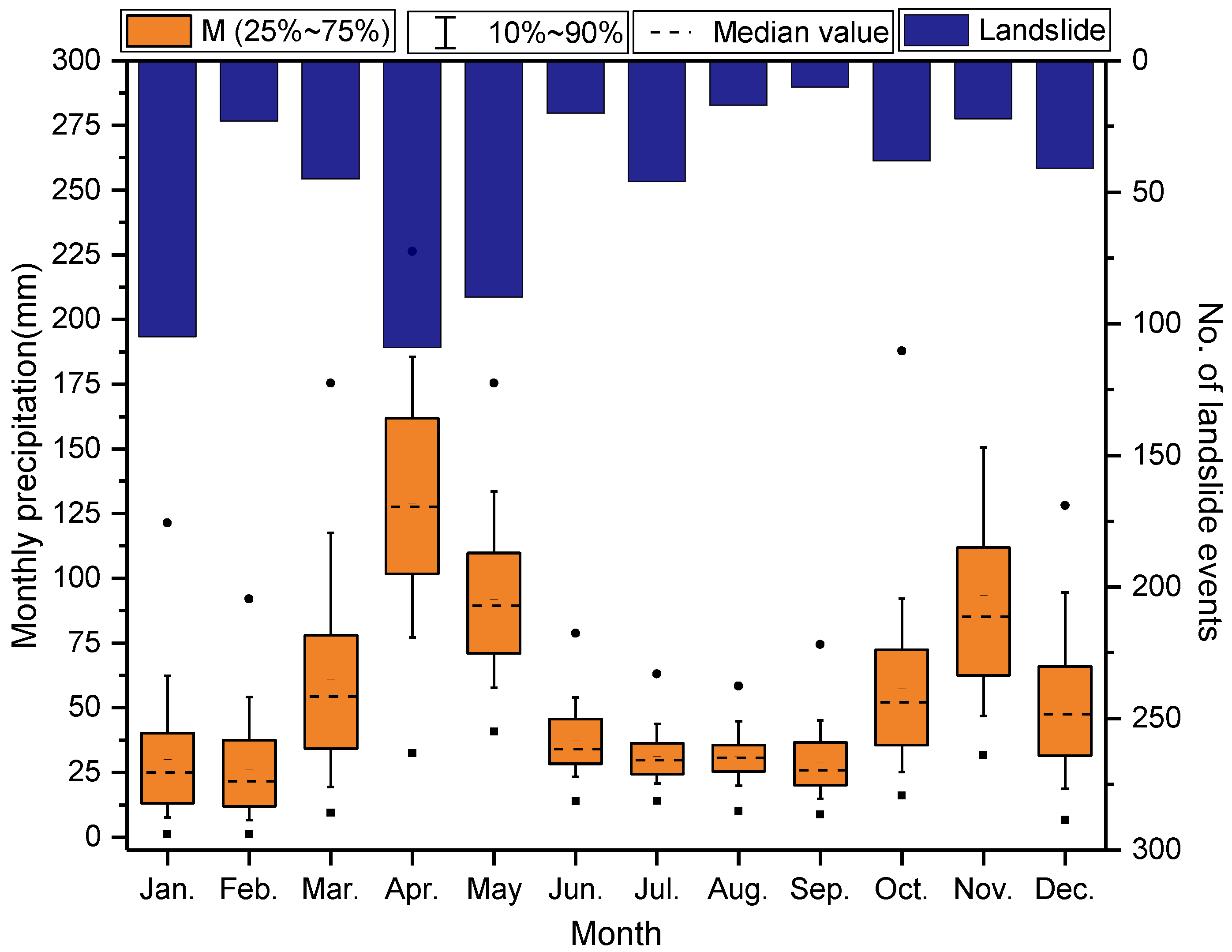
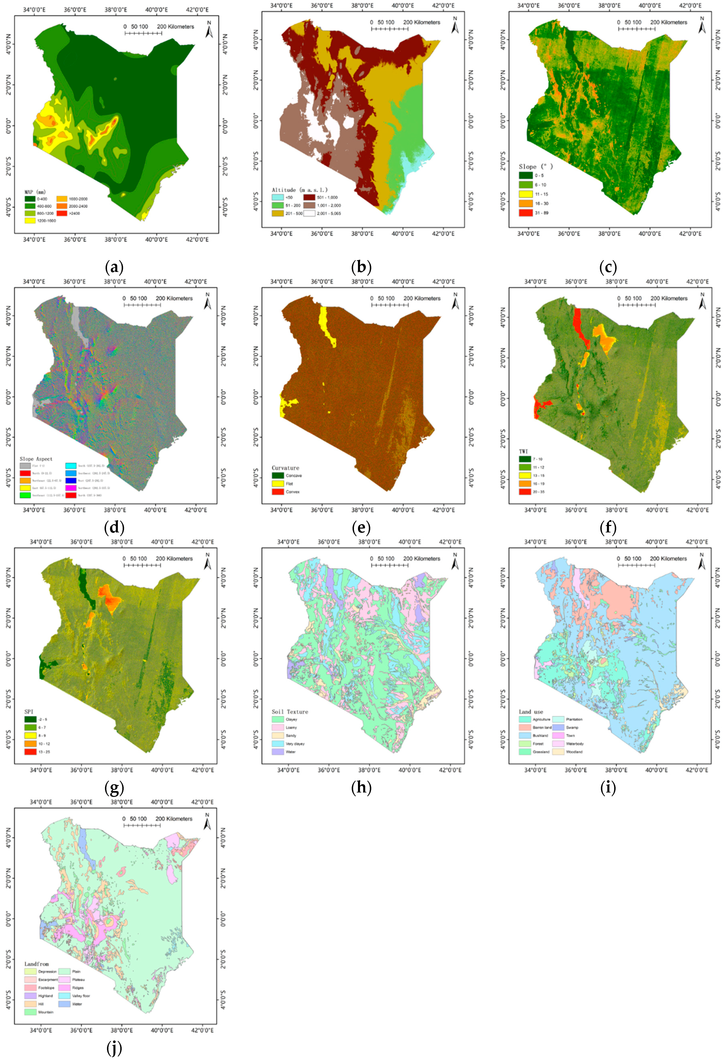
Kenya has a mild climate with annual temperatures ranging from 16 to 26 degrees Celsius. The mean annual precipitation (MAP) in Kenya ranges from <200 mm to 2500 mm. The precipitation of Kenya is characterized by its nonuniform distribution in both time and space. From the historical meteorological data of the Jomo Kenyatta weather station (Figure 2), two distinct rainy seasons can be observed. One is from March to May (the heavy rainy season), and the other is from October to December (the light rainy season). The rest is the dry season. The spatial distribution of MAP is illustrated in Figure 3a. Because of the sudden elevation changes in the GRV zone (from highland to valley then to highland again), there is a sharp transition between wet and dry regions across the GRV zone in southwestern Kenya. Both sides of the GRV in this region had the highest value of MAP, while the northeastern and northern parts of Kenya had the lowest MAP of less than 800 mm. Kenya has experienced a series of geohazards arising from floods, storms, landslides, and debris/mudflows. Most of these geohazards are related to climate extremes [18,20]. Rainfall and human activities (farming, devegetation, construction, etc.) have triggered the majority of the landslides that have occurred in Kenya.

3. Materials

3.1. Historical Landslides in Kenya

A landslide inventory usually portrays the date, location, cause, type, and geometry of landslides. A detailed landslide inventory is a mandatory input for LSM using quantitative methods. Landslide inventories can be produced through field surveys, review of relevant documents, and remote sensing (satellite images, aerial photos, etc.). Since compiling a detailed landslide inventory remains a time- and labor-consuming task there has been no reliable landslide inventory with national coverage available in Kenya until now.
Considering the conditions mentioned above, the landslide inventory utilized in the present study was composed of three subsets from different sources, as illustrated in Figure 1. The first subinventory (LS1) was obtained from the Kenya Open Data of the Ministry of Information, Communications, and Technology of Kenya. LS1 contained 39 historical landslides that occurred in Kenya during the 1999–2013 period. Landslide information regarding the specific longitude/latitude, dates of occurrence, number of people affected, and estimated economic losses were provided in the LS1. The second subinventory (LS2) was derived from the global fatal landslide database (GFLD) (version 2) extracted from Froude and Petley [28]. Similar to LS1, LS2 also provided the location, date of landslide occurrence, induced fatalities, general description, and related reports of landslides. In total, 63 landslides were recorded in LS2. The third subinventory (LS3) was extracted from a landslide inventory of Africa, which was compiled by Broeckx et al. [29]. Within Kenya’s territory, 323 landslides were detected in LS3. The majority of landslides in LS3 were mapped through visual interpretation of Google Earth imagery. This was time-consuming work and involved subjective interpretation. In contrast to LS1 and LS2, only the locations of landslides were provided in LS3. For the present study, a total of 425 landslides were stored in the inventory.
As indicated in Figure 2, the landslide occurrences were mostly concentrated in the periods from April to May and from November to December. It should also be noted that the monthly distribution of landslides was consistent with the monthly distribution of precipitation.

3.2. Landslide Contributing Factors (LCFs)

From the perspective of geotechnical engineering, landslides are a comprehensive consequence of several contributing factors. Nevertheless, there are no global rules for selecting these factors. In a typical LSM, such LCFs are chosen on the basis of data availability, characteristics and scale of the study area, as well as the expert knowledge or experience. In this study, ten LCFs were utilized in LSM over a nationwide area of Kenya, including four topographic factors (namely, the altitude, aspect, slope, and curvature), two hydrological factors (namely, the topographic wetness index (TWI), stream power index (SPI)), soil texture, precipitation, land use, and landform (as shown in Figure 3). To perform the LSM, all factors were rasterized into 1 × 1 km grids and classified into several classes using ArcGIS software (Version 10.2). In what follows, a brief description of each landslide contributing factor is given.

3.2.1. Mean Annual Precipitation (MAP)

Rainfall is among the dominant inducing factors for landslides not only in Kenya but also in many countries because it increases the soil mass and decreases the soil shear strength. As shown in Figure 2, there are strong correlations between landslide occurrences and precipitation in Kenya. For this study, the MAP data were adopted and categorized into nine levels using a 400 mm interval, as shown in Figure 3a. To initially obtain the MAP factor, monthly total rainfall data from 87 meteorological stations in Kenya were collected and filtered. Only data from stations operated in all types of weather were kept. Then, the filtered monthly rainfall data were summed and averaged annually for each station. Finally, through the inverse distance weighting (IDW) of data for each station, the MAP map of Kenya was derived.

3.2.2. Topographic Factors

Topographic factors are most frequently used in LSM. In this study, several topographic factors were created using a 12.5-m digital elevation model (DEM) obtained from the Alaska Satellite Facility (ASF) [30], which included altitude, slope gradient, slope aspect, and curvature information. Because of variations in temperature, humidity, and vegetation, the degree and type of weathering also varied with altitude. Therefore, altitude has been employed as an LCF in previous studies [8,13,15]. Considering the setting of geomorphology and landforms present in Kenya, the altitude factor was categorized as (1) <50 m, (2) 50–200 m, (3) 200–500 m, (4) 500–1000 m, (5) 1000–2000 m, and (6) >2000 m (Figure 3b). Steepness directly affects slope stability because slopes become more susceptible to landslides as the slope gradient increases. Reviews of LSM studies have suggested that the slope gradient factors is usually categorized using a 5° interval. Thus, the slope LCF was categorized as follows: <5°, 5–10°, 10–15°, 15–20°, 20–25°, 25–30°, 30–35°, 35–40°, and >40° (Figure 3c). Since parameters such as sunlight, precipitation, and vegetation cover vary, slope aspects may also have an effect on landslide occurrences. Consistent with previous studies [15,16,31], the aspect factor was classified into 9 subclasses, as shown in Figure 3d. By controlling the water flow and erosion type in curved terrains, curvature is also a commonly used topographic factor that is associated with landslides. A positive curvature value indicates an upwardly convex terrain, while a negative value indicates an upwardly concave terrain. Terrains with values of zero for the curvature factor were classified as flat (Figure 3e).

3.2.3. Hydrological Factors

Hydrological factors played a determinant role in affecting slope stability. For this study, the TWI and the SPI were utilized as predictors of landslides. Both the TWI and the SPI are secondary attributes of the DEM and can be calculated using Equations (1) and (2), respectively. The TWI measures the topographic control on groundwater flow and accumulation. Terrains with a higher TWI values are more likely to become saturated during rainfall events. The SPI quantifies the erosion power of flowing water. Gullies are more likely to form at locations with high SPI values. As indicated in Figure 3f,g, the TWI of the study area ranged from 6.80 to 34.72, and the SPI ranged from −2.41 to 25.13. The factors of TWI and SPI were finally divided into five categories through the “natural breaks” function in GIS.
TWI = ln ( A tan β )
SPI = ln ( A · tan β )
where A is the unit upstream accumulation area, β is the slope gradient, and ln is the natural logarithm.

3.2.4. Environmental Factors

Given the poor data availability in Kenya, three environmental LCFs were considered in this study to produce LS maps. These two factors were soil texture and land use. Soil texture indicates the proportional composition of sand, silt, and clay content in the soil. Because high clay soils usually contain high organic matter content, which is favorable for soil resistance against detachment, soils characterized by high sand or loam content are more susceptible to land sliding than clayey soils [32]. A nationwide soil property GIS database developed by the International Soil Reference and Information Centre (ISRIC) [33] was utilized in this study. Types of soil texture were classified as follows: (1) very clayed, (2) clayed, (3) loamy, and (4) sandy (Figure 3h). Land use and landform type contribute significantly to slope stability. Specifically, vegetation roots may enhance slope stability by altering the cohesive forces and hydrologic properties. The degradation of forests and vegetation increases the degree of susceptibility of the area to landslides [34]. As for the factor of landform, steep and hill/mountain terrains are prone to landslides compared with flat terrains such as plains, valley floor and foot slope. In addition, from the perspective of geomorphology, landslide itself also plays as a driving role in landform evolution [35,36]. The Kenya National Land Use Dataset (KNLD) [37] was utilized in this study to obtain the LCFs of land use and landform type. As indicated in Figure 3i, the KNLD contains ten land use types (Figure 3i) and eleven landform types (Figure 3j).

4. Methodology

A hybrid model of the conventional AHP and fuzzy theory was utilized to conduct the LSM in this study. The AHP has shown good capacity in solving a multicriteria decision-making problem by incorporating expert knowledge into quantitative analysis. To reduce subjectifies involved in conventional AHP analysis, the fuzzy set theory was adopted to handle blurry sets or categories. Hence, the hybrid use of fuzzy sets and conventional AHPs effectively addresses the decision-making issues under multiple criteria. The theoretical background of the conventional AHP and fuzzy theory were briefly introduced in Section 4.1 and Section 4.2, respectively. After that, the process of incorporating fuzzy theory into AHP was given in Section 4.3.

4.1. The Theoretical Background of the Conventional AHP

The AHP, originally developed by Saaty [38], has shown great potential for handling multicriteria decision-making (MCDM) issues. Implemented in GIS, the AHP has been successfully employed in LSM in many previous studies [13,29,31]. A detailed description of the AHP application steps in LSM was introduced by Van et al. [31] and can be summarized as follows:
  • Step 1: Dividing the decision problem into a hierarchical structure
In this step, a complex decision problem was decomposed into a hierarchical structure, including an “objective” level on the top, one or more “criterion” level(s) in the middle, and several decision alternatives at the bottom level. Although there are no universal rules to be followed in constructing such a hierarchy, it was suggested by Saaty [39] that the hierarchy be built based on the decision maker’s knowledge and experience with the problem.
  • Step 2: Constructing the pairwise comparison matrix
In this step, a comparison matrix was constructed with each element indicating the pairwise comparison between all the decision elements. By asking the decision maker how important alternative A is compared to alternative B, the pairwise comparison results (relative importance) are usually rated using a linguistic variable, such as “Slightly Important”, “Moderately Important”, or “Extremely Important” (Table 2).
  • Step 3: Calculate the weights of each decision element and check its consistency
For each comparison matrix, the relative weights of each decision element were calculated using the eigenvalue method (or some other methods). Weights could be used only if consistency had been satisfied.
  • Step 4: Hierarchically aggregate weights from all “criterion” levels
In this step, the score of each alternative with respect to the final goal was calculated by aggregating the weights of decision elements’ weights from all “criterion” levels.
The numerical intensity scale for the relative importance between two decision elements, proposed by Saaty [40], has been broadly used in the AHP. Table 2 shows that in this study, the importance of “Equally Important” to “Extremely Important” was scaled from 1 to 9. The numbers 2, 4, 6, and 8 were used to describe intermediate importance. Inverse importance was scaled using the reciprocals of the numbers from 1 to 1/9. The eigenvalue method was adopted to calculate the weights. In this regard, the consistency index (CI) was calculated as follows:
C I = λ max n n 1
where λmax represents the largest eigenvalue of a matrix.
For evaluation of the CI, the term consistency ratio (CR) was introduced. The CR was defined as the ratio of a given CI and that of a randomly generated reciprocal matrix (RI). Consistency is satisfied if CR < 0.1.
C R = C I R I

4.2. Triangular Fuzzy Number (TFN)

In the practical application of the conventional AHP for LSM, the determination of the exact relative importance of two factors (A and B) is more difficult than to identify one factor as being more important to another. Given this, fuzzy theory was employed to extend the conventional AHP by scaling the experts’ decisions as fuzzy numbers. Thus, assigning exact ratio values to pairwise comparison results was avoided. There are many types of fuzzy numbers. For this study, triangular fuzzy numbers (TFNs) were used. Concepts for the TFN-AHP are briefly introduced in the following.
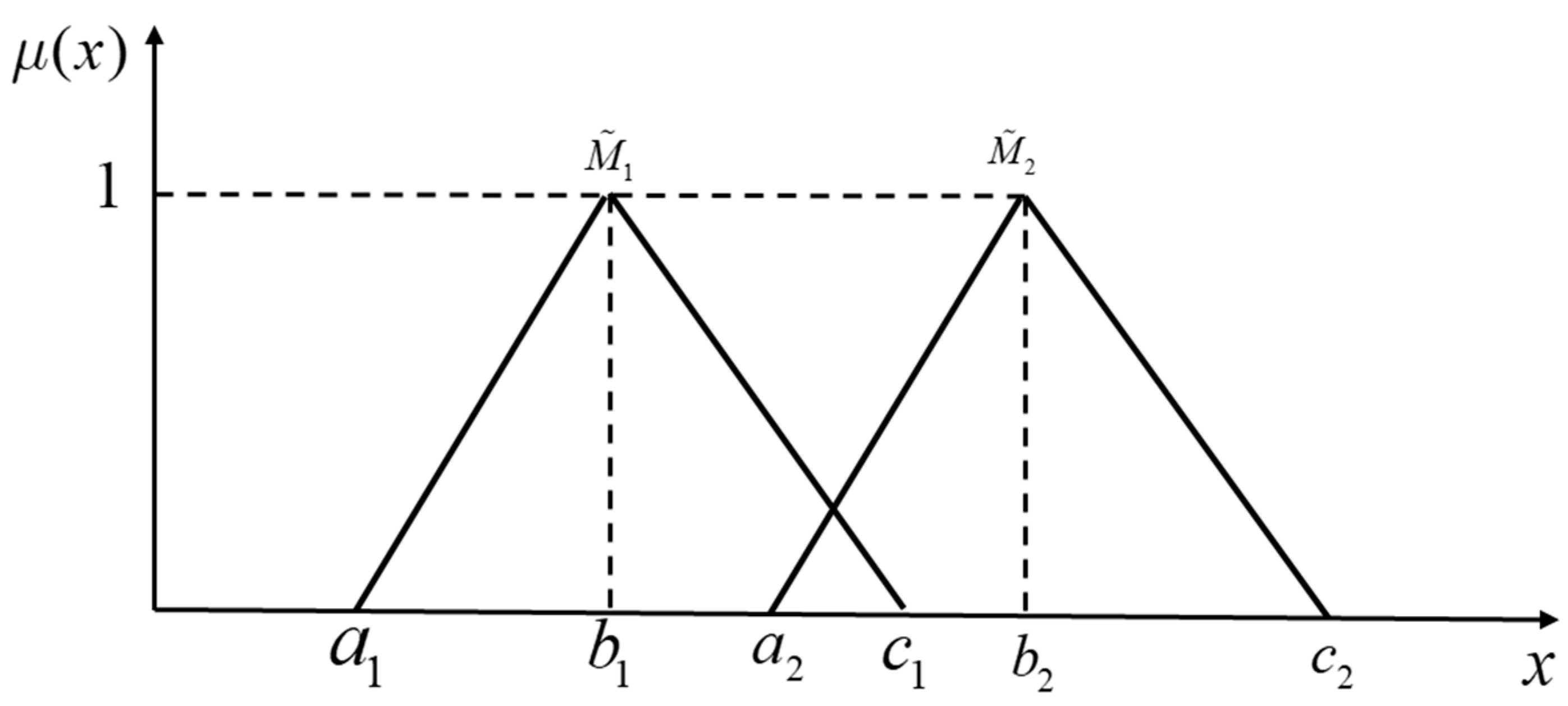
Let M ˜ be a TFN on R; then, its member function x M ˜ , μ M ( x ) : R [ 0 , 1 ] can be defined as follows:
μ M ( x ) { 0 x < a   or   x > c   ( x a ) / ( b a ) , a x b ( c x ) / ( c b ) , b x c
where a, b, and c represent the left, modal, and right values of M ˜ , respectively (see Figure 4).
A TFN can be denoted by M ˜ = ( a , b , c ) . Let M ˜ 1 = ( a 1 , b 1 , c 1 ) and M ˜ 2 = ( a 2 , b 2 , c 2 ) be two TFNs, where a 1 , a 2 > 0 , b 1 , b 2 > 0   and   c 1 , c 1 > 0 . The laws of the operations can be defined as follows:
  • Summation of two TFNs:
    M ˜ 1 M ˜ 2 = ( a 1 + a 2 , b 1 + b 2 , c 1 + c 2 )
  • Subtraction of a TFN from another TFN:
    M ˜ 1 Θ M ˜ 2 = ( a 1 - a 2 , b 1 - b 2 , c 1 - c 2 )
  • Multiplication of two TFNs:
    M ˜ 1 M ˜ 2 = ( a 1 × a 2 , b 1 × b 2 , c 1 × c 2 )
  • Multiplication of a number and a TFN:
    λ M ˜ 1 = ( λ × a 1 , λ × b 1 , λ × c 1 )
  • Division of a TFN by another TFN:
    M ˜ 1 Ø M ˜ 2 = ( a 1 , b 1 , c 1 ) Ø ( a 2 , b 2 , c 2 ) = ( a 1 c 2 , b 1 b 2 , c 1 a 2 )
  • Reciprocal of a TFN:
    M ˜ 1 1 = ( a 1 , b 1 , c 1 ) 1 = ( 1 c 1 , 1 b 1 , 1 a 1 )

4.3. Integration of the AHP and TFN

The integration of fuzzy sets with the AHP has shown great potential not only for use in LSM but also in many other multicriteria decision making processes, such as hospital location selection and tourist risk evaluation. Very reliable results have been obtained in these applications. The following sections will describe the TFN-AHP theory.
In TFN-AHP theory, experts’ judgments are scaled using a TFN rather than a definite number. Then, the TFN comparison matrix is defined as follows:
K ˜ = ( k ˜ i j ) n × n = [ 1 ˜ k ˜ 12 k ˜ 1 n k ˜ 21 1 ˜ k ˜ 2 n k ˜ n 1 k ˜ n 2 1 ˜ ] = [ 1 ˜ k ˜ 12 k ˜ 1 n k ˜ 12 - 1 1 ˜ k ˜ 2 n k ˜ 1 n - 1 k ˜ 2 n - 1 1 ˜ ]
where k ˜ i j = ( a i j , b i j , c i j ) denotes the fuzzy comparison value of criterion i to criterion j and k ˜ i j 1 = ( 1 c i j , 1 b i j , 1 a i j ) denotes the reciprocal value for i , j = 1 , 2 , , n and i j .
If such judgments are made by consulting more than one expert, the element value is calculated by the average of their decisions as follows:
k i j = 1 h ( k i j 1 + k i j 1 + + k i j 1 )
where k i j p = [ l i j p , m i j p , u i j p ]   p [ 1 , 2 , , h ] and h is the number of experts.
Consistent with Chang (1996) [41], the required steps to compute the weight vector for a TFN comparison matrix can be expressed using the following procedure:
First, calculate the fuzzy synthetic extent with respect to the ith alternative by normalization of the row sums of the fuzzy comparison matrix as follows:
S ˜ i = j = 1 n k ˜ i j [ l = 1 n j = 1 n k ˜ l j ] 1 ,   i = 1 , 2 , , n
Then, calculate weight vectors concerning each decision element under a certain criterion using the degree of possibility of M ˜ i M ˜ j , which is defined as follows:
V ( M ˜ i M ˜ j ) = sup y x { min [ M ˜ j ( x ) , M ˜ i ( y ) ] }
This equation can be equivalently expressed as follows:
V ( M ˜ i M ˜ j ) = { 1 b i b j c i - a j ( c i b i ) + ( b j a j ) a j c i 0 otherwise
Finally, calculate the normalized vector of weights W ˜ = ( w ˜ 1 , w ˜ 2 , , w ˜ n ) of the TFN comparison matrix K ˜ as follows:
w i = V ( M ˜ i M ˜ j | j = 1 , 2 , , n ; i j ) k = 1 n V ( M ˜ i M ˜ j | j = 1 , 2 , , n ; i j )
The typical LSM is performed based on raster cells. For the TFN-AHP application in LSM, the criteria refer to a series of LCFs, whereas the alternatives refer to the raster cells within the study area. To perform the LSM using the TFH-AHP, a weighted linear combination (WLC) is conducted to calculate the LSI for each raster pixel as follows:
LSI = i = 1 n w i s i k ( x , y )
where wi is the weight of ith criterion (LCF) i, s i k ( x , y ) is the weight of the kth subcriteria (subclass for the LCF) in the ith criterion, and k is determined by the spatial location (x, y) of the raster cell.

4.4. Accuracy Validation

A review of the literature has shown that the receiver operating characteristic (ROC) curve is a popular method to evaluate the goodness of fit for classification [1,4,5,6,7]. The area under this curve (AUC) is adopted to measure the generalization performance of the LSM model. The value of AUC usually ranges between 0.5 to 1.0. A higher AUC value, closer to 1.0, indicates a better performance of the classification model.
TPR = TP TP + FN
FPR = FP FP + TN
The first step in performing the ROC analysis was to construct the validation dataset, which contained both landslide and non-landslide events. For this study, 425 known landslides were used for validation. Additionally, 425 non-landslides were randomly chosen for validation within the study area. Then, by setting different threshold LSI values, the dataset was separated into four groups according to the actual label and precited label. As shown in Table 3, the four groups were true positive (TP), true negative (TN), false positive (FP), and false-negative (FN) events. After that, two indexes were employed; one was the true positive rate (TPR) computed using Equation (19), and the other was the false positive rate (FPR) computed using Equation (20). Eventually, the ROC curve was drawn by plotting the FPR and the TPR on the horizontal and vertical axes, respectively.

4.5. Flowchart of Conducting the LSM

In general, the process to conduct the LSM using the proposed TFN-AHP method can be summarized as following 5 steps. Firstly, the 10 LCFs (criteria) that were required to perform the LSM were chosen (as described in Section 3). Then, a two-level hierarchical model was developed with 10 criteria and 41 subcriteria. Next, 11 comparison matrices were established to calculate the criteria weights. After that, using a WLC of weights of all levels, an LSI map was created and reclassified. Finally, the accuracy of the obtained map was validated using ROC curve and the known historical landslides.

5. Results

5.1. Weights of LCFs and Their Subclasses

The weighting vector derivation plays a central role in multicriteria decision making. For the present study, weights were assigned to each LCF. For this purpose, the geotechnical experts were called upon to make a pairwise comparison of the LCFs based on their experiences and knowledge. As illustrated in Table 4, the pairwise comparison matrix for the ten LCFs was constructed by considering expert opinion and similar previous studies [21,22,23,26,27]. From the matrix, the weight vector for the criteria was computed using Equation (14) to Equation (17) and is presented in Table 5. After normalization, the weights for each criterion were derived using Equation (18) and are shown in Table 6. The CR was calculated using Equations (3) and (4). When the CR = 0.086 < 0.1, the judgment was deemed to be consistent.
For the subcriteria (subclasses) under a certain uplevel criterion (an LCF), the weights were derived using the same procedures. The sum of subcriteria weights under each corresponding uplevel criterion should be 1.0. Hence, 10 comparison matrices were created. Additionally, the final weights for the subclasses within each LCF were calculated and are shown in Table 6. Before using these calculated weights, a consistency check was conducted for each comparison matrix. Only if CR < 0.1 was the derived weight accepted. Since all CR values were less than 0.1 (Table 6), a consistency check of the 10 matrices indicated that all the judgments were consistent.
From the TFN-AHP analysis, slope gradient (0.1923), MAP (0.1884), and curvature (0.1651) were considered to be the three most important factors contributing to landslide occurrence, whereas the least important factors were land use (0.0220) and aspect (0.0315). For the factor of slope gradient, the terrain steeper than 30° was most susceptible to landslides (weight for this subclass is 0.364313), while the category of 5–10° obtained the lowest weights (0.071825) in determining the landslide occurrences. It also can be seen from results that barren land (0.160743), bush land (0.136464), and grassland (0.121685) were most susceptible to landslides compared with other land use types. In case of curvature, both concave and convex terrain were more prone to landsliding than flat area. Convex terrain (subclass weight is 0.570014) was more favorable for landsliding than concave terrains (0.356956).

5.2. Landslide Susceptibility Maps

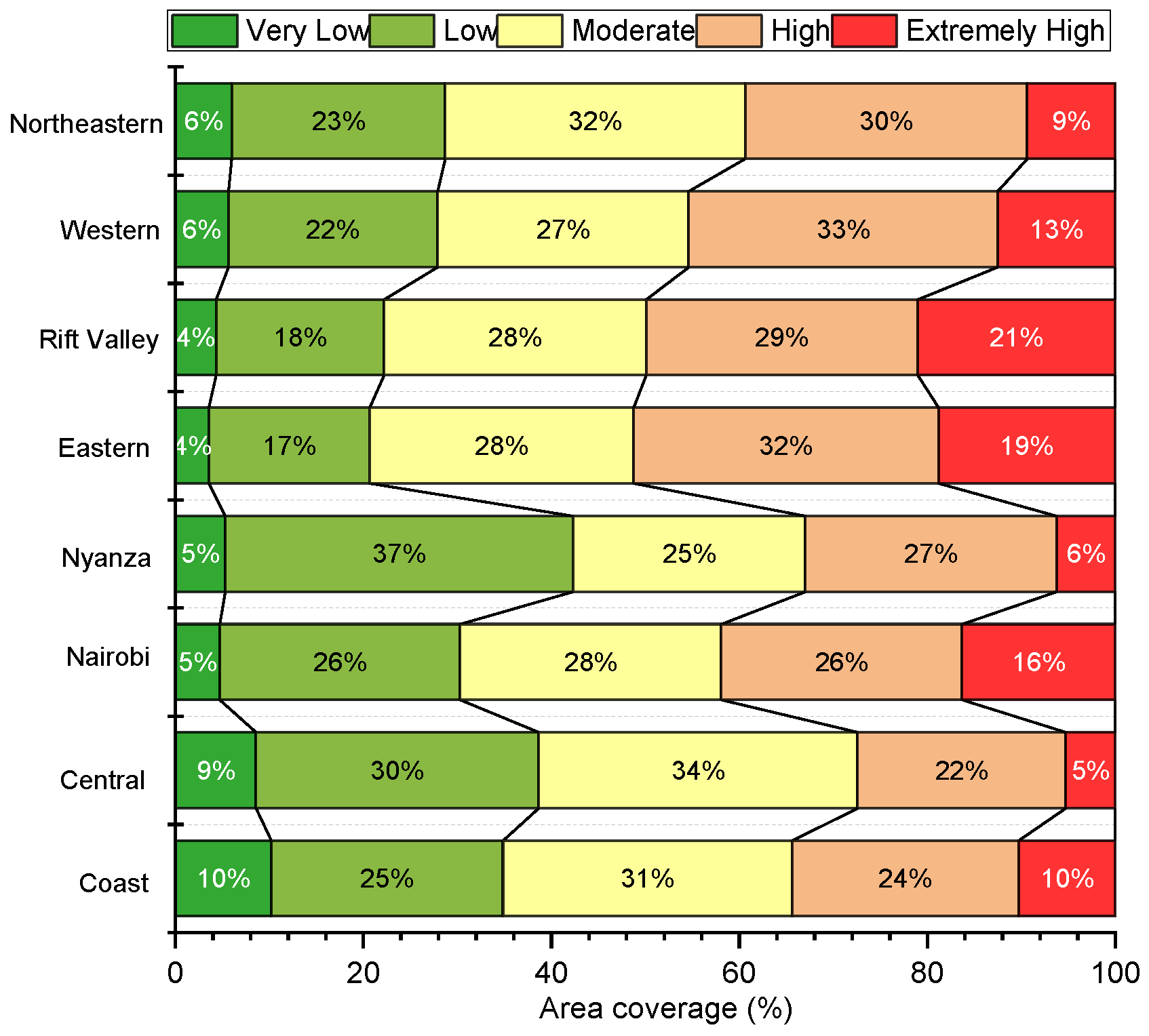
Using Equation (18), the LSI value for each raster cell within Kenya was calculated. As shown in Figure 5, the resultant LSI map was reclassified into five susceptibility levels using the “natural break” function ArcGIS. In total, 15.44% and 29.16% of the Kenyan territory were mapped as extremely high susceptibility zones. A total of 29.16% of the total area was predicted as a high susceptibility zone. Low and very low susceptibility classes covered 20.58% and 5.53% of the study area, respectively. The remaining 29.29% of the study area was determined to be moderately susceptible to landslides (Figure 6). The distribution of susceptibility classes differed in each province. As illustrated in Figure 7, the Rift Valley Province and Eastern Province had the highest percentages of EH landslide susceptibility coverage (21% and 19%, respectively), while the Central Province and Nyanza Province had the lowest percentages of EH landslide susceptibility (5% and 6%, respectively).

5.3. Accuracy Validation

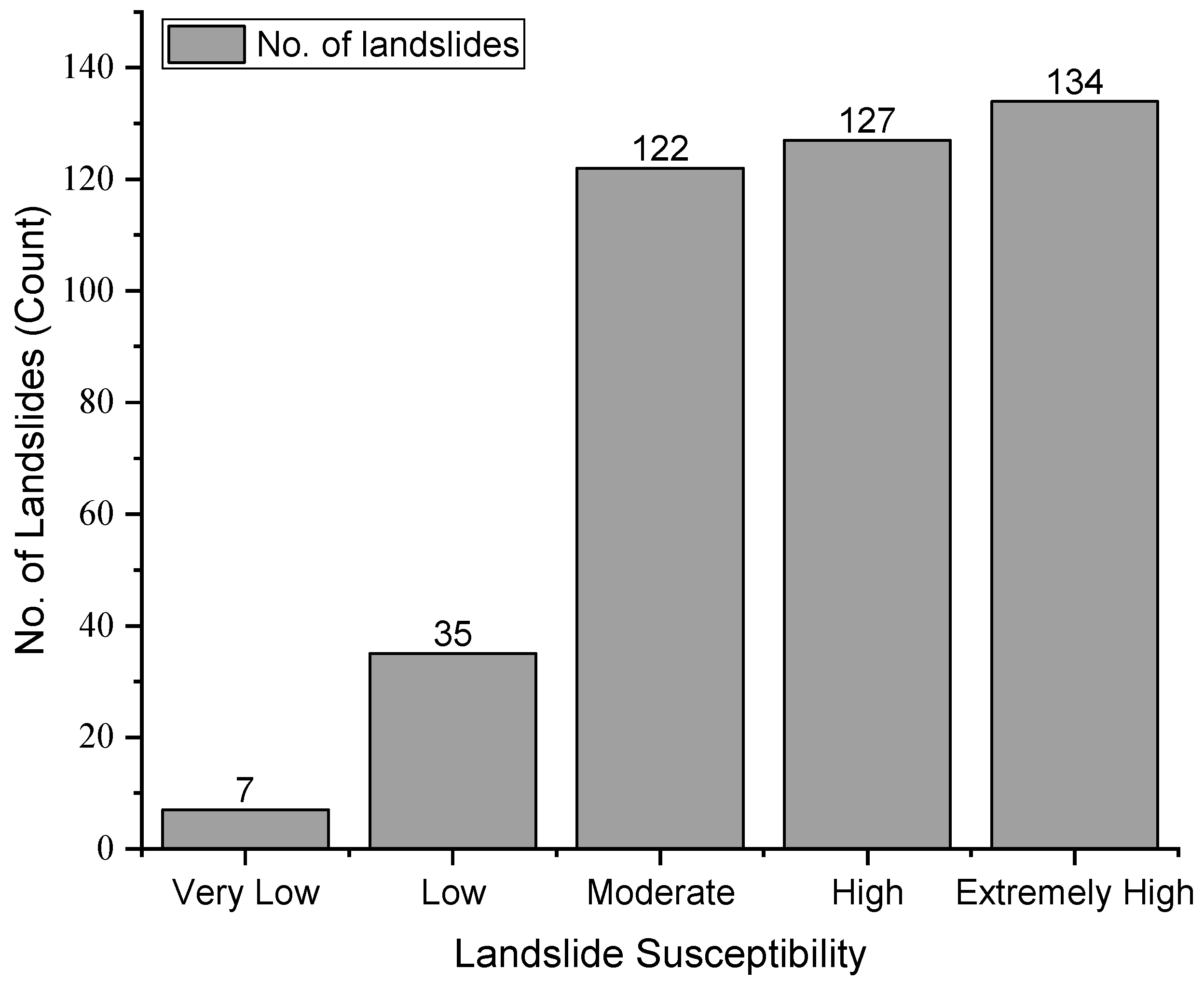
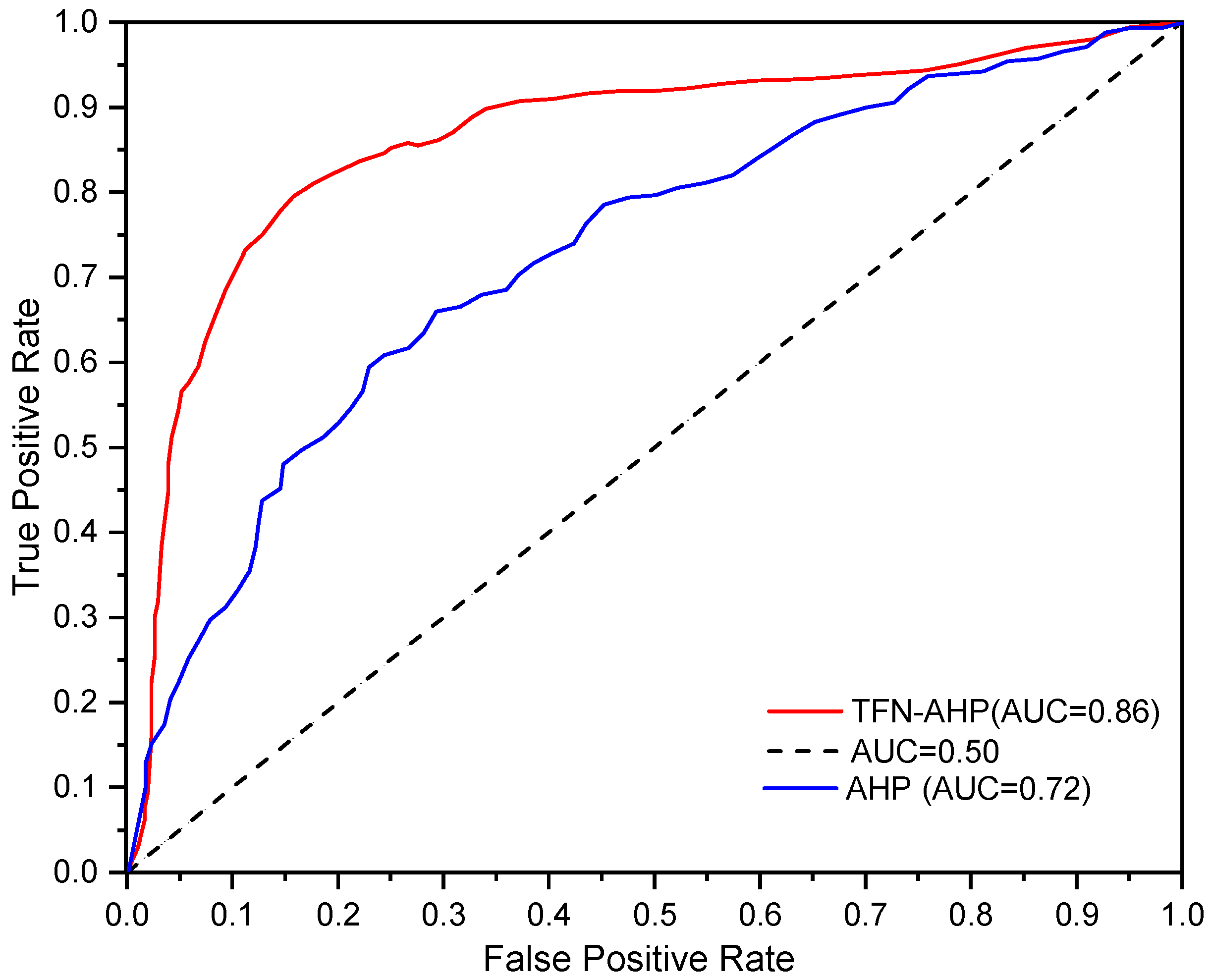
Figure 8 shows that over 60% of the landslides had occurred in the extremely high (31.53%, 134 of 425) and high (29.88%, 127 of 425) landslide susceptibility areas, respectively. Less than 10% of the total landslides occurred in the area mapped as low (8.24%, 35 of 425) and very low (1.65%, 7 of 425) susceptibility levels. In line with the procedures described in Section 4.5, the ROC curve was drawn as shown in Figure 9, and the AUC value was 0.86.

6. Discussion

This research was proposed to apply the TFN-AHP method to map landslide susceptibility in Kenya. Figure 5 directly displays the visible landslide susceptibility information for the entire Kenyan territory, indicating the likelihood of potential landslides. As a developing country, such information would greatly benefit Kenyan efforts to minimize landslide-induced losses and develop optimized land management policies. From Figure 6, it was observed that 44.6% of Kenya is classified as high- and extremely high-susceptibility zones, whereas 26.11% of Kenya was mapped as having low and very low susceptibility. High and extremely high landslide susceptibility zones predominantly cover the rift valley region and its surrounding areas. This finding can be attributed to plentiful rainfall, steep terrains, and fractured ground. Low and very low landslide susceptibility areas are primarily distributed in the southwestern and coastal regions. The distribution of susceptibility classifications also varies in different provinces (Figure 7). The Rift Valley Province had a majority of the historical landslides. This province has the largest area coverage of extremely high- and high-susceptibility zones.
Dozens of methods have been used in LSM at different scales. For large areas with poor availability of historical landslide inventories, the spatial multicriteria evaluation (SMCE) method has exhibited overwhelming advantages over statistical and the physically based methods [15,42]. As a representative SMCE method, a review of previous studies (as displayed in Table 1) has suggested that the AHP and its fuzzy extensions are one of the favorable methods in LSM for large areas (e.g., for a whole country). One limitation of the application of the statistical method in this study is the incompleteness of the historical landslide inventory, which reduces the reliability of the results. Despite this, the historical landslide inventory can still be used for validation in a better than no sense.
The validation results demonstrate that the adopted TFN-AHP resulted in promising accuracy with an AUC value of 0.86 (Figure 9). Despite no strict rules for the evaluation of this accuracy, the resultant accuracy seems to be good compared to similar studies in different areas [1,3,8]. For the LSM, an ideal result map should include as many historical landslides as possible in “high” or “extremely high” susceptibility regions. Additionally, few historical landslides should occur in the “low” or “very low” susceptibility region. Figure 8 shows that the concentration of known landslides decreases from the extremely high category to the very low category. For decision making under multiple criteria, it is difficult for humans to quantify criteria weights using extract numbers. However, rational decisions can be made by skilled experts through a certain value with some uncertainties to capture human subjectivity. Given this, the TFN-AHP makes the comparison process more flexible to minimize the objectivities and uncertainties involved in the conventional AHP process. For the purpose of comparison, the map produced using the conventional AHP is illustrated in Figure 10. The ROC analysis, with an AUC value of 0.72, is also plotted in Figure 9. To perform the conventional AHP, the element value of the TFN-AHP comparison matrix is replaced by a single number according to Table 2. The comparison matrix for the conventional AHP analysis is shown in Appendix A. It should be noted that another source of the subjectivities involved in this study and other similar studies using the SMCE methods or statistical methods may originate from the selection of the LCFs. As shown in Table 1, the number of factors used for LSM ranges from 3 to 10. As discussed in many case studies [1,5,9,16,25,27] and more recently reviewed in [13], the selection of LCFs largely depends on conditions such as data availability, scale, and nature of the study area.
Even for skilled departments from China and many other developing countries, no universal rules have been proposed. Hence, for a given study area, comparative studies have always been conducted to select the best maps.

7. Conclusions

In this research, an integrated method of fuzzy theory and conventional AHP analysis was employed for the LSM of Kenya. A two-level hierarchical index system was established to predict landslide susceptibility with a GIS platform. Ten factors contributing to landslide occurrence were included in the first level of the evaluation system. These contributing factors included slope, altitude, aspect, SPI, TWI, curvature, land use, MAP, landform, and soil texture. For the second level, each of these factors was divided into several subclasses. The weights of these factors and their subclasses were determined using the adopted TFN-AHP theory. A nationwide landslide susceptibility map for the entire Kenyan territory was produced with five different levels ranging from extremely high susceptibility to very low susceptibility. Extremely high and high landslide susceptibility zones primarily covered the rift valley and its nearby regions. Validation results using ROC curves indicated that the TFN-AHP method performed well for developing LS maps of the study area. This method resulted in a higher AUC accuracy than the conventional AHP using the same datasets.
This study was the first attempt to identify landslide susceptibility zones in Kenya on a national scale. The produced map can be used as a general indicator of the relative landslide susceptibility for larger areas rather than an accurate susceptibility measure for each specific site. The results would be helpful in various land resources-related fields to inform decision making, such as regional landslide hazard mitigation, land use management, and infrastructure planning.

Author Contributions

X.T. contributed to the conception of the study, S.Z. (Suhua Zhou) performed the data analyses. S.Z. (Shuaikang Zhou) wrote the manuscript. All authors have read and agreed to the published version of the manuscript.

Funding

This work was supported by the National Natural Science Foundation of China (grant number 51708199); the Science and Technology Infrastructure Program of Guizhou Province (grant number 2020-4Y047: 2018-133-042); the Fundamental Research Funds for the Central Universities (grant number 531107050969); the Science and Technology Program of Beijing (grant number Z181100003918005). All these financial supports were acknowledged.

Acknowledgments

The authors would like to express their gratitude to Fang and Li Hongquan in Central South University for their kind help in evaluating the LCFs.

Conflicts of Interest

The authors declare no conflict of interest.

Appendix A

Table A1. Pairwise comparison matrix and normalized weight of ten LCFs using the conventional AHP.
LCFLanduseAMPAspectSoil TextureTWISPICurvatureAltitudeLandformSlopew
Landuse11/221/21/21/21/41/21/21/40.0455
AMP21233323430.2073
Aspect1/21/211/21/21/21/221/21/30.0552
Soil Texture21/321221/31/531/40.0776
TWI21/321/2111/2231/40.0786
SPI21/321/2111/21/221/50.0615
Curvature41/2232212320.1527
Altitude21/31/251/221/2121/40.0914
Landform21/421/31/31/21/31/211/20.0498
Slope41/334451/24210.1803
Table A2. Weights for subclasses within each LCF calculated using the conventional AHP.
LCFSubclassSubclass IndicatorC1C2C3C4C5C6C7C8C9C10w
Altitude
(CR = 0.0561)
<50C111/211/51/41 0.0835
50–200C2211/21/31/210.1094
200–500C31211/211/20.1385
500–1000C45321220.3209
1000–2000C54211/2120.2104
>2000C61121/21/210.1374
Slope
(CR = 0.0665)
0–5C112131/2 0.2357
5–10C21/2111/31/30.1010
10–15C311111/30.1438
15–30C41/33111/20.1634
>30C5233210.3561
Aspect
(CR = 0.0983)
EastC111/31/2221/31/21/21/4 0.0642
NorthC231322211/31/20.1316
SouthC321/312131/21/31/30.0894
FlatC41/21/21/2111/31/311/40.0544
SoutheastC51/21/211111/321/20.0838
NortheastC631/21/33111/211/30.0892
NorthwestC7212332111/20.1396
SouthwestC823311/211110.1442
WestC94234232110.2036
Curvature
(CR = 0.0028)
ConcaveC1121/2 0.2970
FlatC21/211/30.1634
ConvexC32310.5396
TWI
(CR = 0.0261)
6.8–9.87C11211/21/2 0.1635
9.88–12.06C21/2111/21/20.1234
12.07–14.68C31111/21/20.1394
14.69–18.73C422211/20.2468
18.74–34.72C5222210.3270
SPI
(CR = 0.0738)
−2.41–4.61C1111/211/2 0.1370
4.62–6.66C2111/21/21/30.1069
6.67–9.04C32211/210.2152
9.05–12.28C412211/30.2076
12.29–25.13C5231310.3333
Soil Texture
(CR = 0.0366)
VeryclayedC112323 0.3692
ClayedC21/212120.2085
LoamyC31/31/211/21/20.0958
SandyC41/212110.1796
WaterC51/31/22110.1469
Landuse
(CR = 0.0929)
GrasslandC111/31/212113320.1146
BarrenlandC231232322320.1905
BushlandC321/2121232220.1379
WaterbodyC411/31/211/21/221/21/310.0618
PlantationC51/21/21211221/220.0990
AgricultureC611/31/221111310.0891
TownC711/21/31/21/211221/30.0741
ForrestC81/31/21/221/211/21230.0854
SwampC91/31/31/2321/31/21/211/20.0686
WoodlandC101/21/21/211/2131/3210.0790
Landform
(CR = 0.0999)
DepressionC111/33221/241/3330.1192
EscarpmentC231322141320.1609
WaterC31/31/311/21/21/421/511/20.0433
HighlandC41/21/22111/331/4220.0794
HillC51/21/22111/331/421/20.0693
MountainC621433131/231/20.1434
PlainC71/41/41/21/31/31/311120.0573
RidgesC831544211330.1989
ValleyfloorC91/31/311/21/21/311/3120.0518
FootslopeC101/31/221/2221/21/31/210.0766
AMP
(CR = 0.0931)
0–400C111221/321/2 0.1425
400–800C2111321/31/20.1350
800–1200C31/2111/21/21/31/30.0683
1200–1600C41/21/3211/21/31/30.0700
1600–2000C531/222111/30.1541
2000–2400C61/23331110.1901
>2400C722333110.2400

References

  1. Pham, B.T.; Shirzadi, A.; Bui, D.T.; Prakash, I.; Dholakia, M. A hybrid machine learning ensemble approach based on a radial basis function neural network and rotation forest for landslide susceptibility modeling: A case study in the Himalayan area. Int. J. Sediment Res. 2018, 33, 157–170. [Google Scholar] [CrossRef]
  2. Petley, D. Global patterns of loss of life from landslides. Geology 2012, 40, 927–930. [Google Scholar] [CrossRef]
  3. Brabb, E.E. Innovative Approaches to Landslide Hazard Mapping; Landslides: Toronto, ON, Canada, 1984; pp. 307–324. [Google Scholar]
  4. Razandi, Y.; Pourghasemi, H.R.; Neisani, N.S.; Rahmati, O. Application of analytical hierarchy process, frequency ratio, and certainty factor models for groundwater potential mapping using GIS. Earth Sci. Inform. 2015, 8, 867–883. [Google Scholar] [CrossRef]
  5. Son, J.; Suh, J.; Park, H.D. GIS-based landslide susceptibility assessment in Seoul, South Korea, applying the radius of influence to frequency ratio analysis. Environ. Earth Sci. 2016, 75, 310. [Google Scholar] [CrossRef]
  6. Dailey, L.A.; Fuhrmann, S. GIS-Based Logistic Regression for Landslide Susceptibility Analysis in Western Washington State. Int. J. Appl. Geospat. Res. 2017, 8, 1–19. [Google Scholar] [CrossRef] [Green Version]
  7. Hong, H.; Tsangaratos, P.; Ilia, I.; Liu, J.; Zhu, A.-X.; Chen, W. Application of fuzzy weight of evidence and data mining techniques in construction of flood susceptibility map of Poyang County, China. Sci. Total. Environ. 2018, 625, 575–588. [Google Scholar] [CrossRef] [PubMed]
  8. Shahri, A.A.; Spross, J.; Johansson, F.; Larsson, S. Landslide susceptibility hazard map in southwest Sweden using artificial neural network. Catena 2019, 183, 104225. [Google Scholar] [CrossRef]
  9. Zhou, S.; Fang, L. Support vector machine modeling of earthquake-induced landslides susceptibility in central part of Sichuan province. Geoenvironmental Disasters 2015, 2, 117. [Google Scholar] [CrossRef] [Green Version]
  10. Godt, J.; Baum, R.; Savage, W.; Salciarini, D.; Schulz, W.; Harp, E. Transient deterministic shallow landslide modeling: Requirements for susceptibility and hazard assessments in a GIS framework. Eng. Geol. 2008, 102, 214–226. [Google Scholar] [CrossRef]
  11. Oliveira, S.C.; Zêzere, J.L.; Lajas, S.; Melo, R. Combination of statistical and physically based methods to assess shallow slide susceptibility at the basin scale. Nat. Hazards Earth Syst. Sci. 2017, 17, 1091–1109. [Google Scholar] [CrossRef]
  12. Van Westen, C.J.; Castellanos, E.; Kuriakose, S.L. Spatial data for landslide susceptibility, hazard, and vulnerability assessment: An overview. Eng. Geol. 2008, 102, 112–131. [Google Scholar] [CrossRef]
  13. Reichenbach, P.; Rossi, M.; Malamud, B.D.; Mihir, M.; Guzzetti, F. A review of statistically-based landslide susceptibility models. Earth Sci. Rev. 2018, 180, 60–91. [Google Scholar] [CrossRef]
  14. Cabral, G.G.; Oliveira, A.L.I. Artificial Intelligence in Theory and Practice II; Springer Science & Business Media: Santiago, Chile, 2008; pp. 245–254. [Google Scholar]
  15. Barella, C.F.; Sobreira, F.G.; Zêzere, J.L. A comparative analysis of statistical landslide susceptibility mapping in the southeast region of Minas Gerais state. Bull. Int. Assoc. Eng. Geol. 2018, 78, 3205–3221. [Google Scholar] [CrossRef]
  16. Zhu, A.-X.; Miao, Y.; Wang, R.; Zhu, T.; Deng, Y.; Liu, J.; Yang, L.; Qin, C.-Z.; Hong, H. A comparative study of an expert knowledge-based model and two data-driven models for landslide susceptibility mapping. Catena 2018, 166, 317–327. [Google Scholar] [CrossRef]
  17. Davies, T.C. Landslide research in Kenya. J. Afr. Earth Sci. 1996, 23, 541–545. [Google Scholar] [CrossRef]
  18. Paron, P.; Olago, D.O.; Omuto, C.T. Kenya: A Natural Outlook: Geo-Environmental Resources and Hazards; Newnes: Boston, MA, USA, 2013; pp. 293–314. [Google Scholar]
  19. Waithaka, E.H.; Agutu, N.; Mbaka, J.G.; Ngigi, T.G.; Waithaka, E.H. Landslide scar/soil erodibility mapping using Landsat TM/ETM+ bands 7 and 3 normalised difference index: A case study of central region of Kenya. Appl. Geogr. 2015, 64, 108–120. [Google Scholar] [CrossRef] [Green Version]
  20. Ngecu, W.M.; Mathu, E.M. The El-Nino-triggered landslides and their socioeconomic impact on Kenya. Environ. Earth Sci. 1999, 38, 277–284. [Google Scholar] [CrossRef]
  21. Abella, E.A.C.; Van Westen, C.J. Generation of a landslide risk index map for Cuba using spatial multi-criteria evaluation. Landslides 2007, 4, 311–325. [Google Scholar] [CrossRef] [Green Version]
  22. Bălteanu, D.; Chendeş, V.; Sima, M.; Enciu, P. A country-wide spatial assessment of landslide susceptibility in Romania. Geomorphology 2010, 124, 102–112. [Google Scholar] [CrossRef]
  23. Sabatakakis, N.; Koukis, G.; Vassiliades, E.; Lainas, S. Landslide susceptibility zonation in Greece. Nat. Hazards 2012, 65, 523–543. [Google Scholar] [CrossRef]
  24. Margottini, C.; Canuti, P.; Sassa, K. Landslide Science and Practice: Volume 1: Landslide Inventory and Susceptibility and Hazard Zoning; Springer: Berlin/Heidelberg, Germany, 2013; pp. 303–311. [Google Scholar]
  25. Gaprindashvili, G.; Van Westen, C.J. Generation of a national landslide hazard and risk map for the country of Georgia. Nat. Hazards 2015, 80, 69–101. [Google Scholar] [CrossRef]
  26. Okalp, K.; Akgün, H. National level landslide susceptibility assessment of Turkey utilizing public domain dataset. Environ. Earth Sci. 2016, 75, 847. [Google Scholar] [CrossRef]
  27. Nsengiyumva, J.B.; Luo, G.; Nahayo, L.; Huang, X.; Cai, P. Landslide susceptibility assessment using spatial multi-criteria evaluation model in Rwanda. Int. J. Environ. Res. Public Health 2018, 15, 243. [Google Scholar] [CrossRef] [PubMed] [Green Version]
  28. Froude, M.J.; Petley, D.N. Global fatal landslide occurrence from 2004 to 2016. Nat. Hazards Earth Syst. Sci. 2018, 18, 2161–2181. [Google Scholar] [CrossRef] [Green Version]
  29. Broeckx, J.; Vanmaercke, M.; Duchateau, R.; Poesen, J. A data-based landslide susceptibility map of Africa. Earth Sci. Rev. 2018, 185, 102–121. [Google Scholar] [CrossRef]
  30. Alaska Satellite Facility. Available online: www.asf.alaska.edu/ (accessed on 13 December 2020).
  31. Van, N.T.H.; Van Son, P.; Khanh, N.H.; Binh, L.T. Landslide susceptibility mapping by combining the analytical hierarchy process and weighted linear combination methods: A case study in the upper Lo River catchment (Vietnam). Landslides 2016, 13, 1285–1301. [Google Scholar] [CrossRef]
  32. Sharma, L.P.; Patel, N.; Debnath, P.; Ghose, M. Assessing landslide vulnerability from soil characteristics—A GIS-based analysis. Arab. J. Geosci. 2011, 5, 789–796. [Google Scholar] [CrossRef]
  33. ISRIC-World Soil Information. Available online: www.data.isric.org (accessed on 13 December 2020).
  34. Reichenbach, P.; Mondini, A.C.; Rossi, M. The influence of land use change on landslide susceptibility zonation: The Briga catchment test site (Messina, Italy). Environ. Manag. 2014, 54, 1372–1384. [Google Scholar] [CrossRef] [Green Version]
  35. Roering, J. Tectonic geomorphology: Landslides limit mountain relief. Nat. Geosci. 2012, 5, 446–447. [Google Scholar] [CrossRef]
  36. Larsen, I.J.; Montgomery, D.R. Landslide erosion coupled to tectonics and river incision. Nat. Geosci. 2012, 5, 468–473. [Google Scholar] [CrossRef]
  37. ICPAC-Geoportal. Available online: www.geoportal.icpac.net/ (accessed on 13 December 2020).
  38. Saaty, T.L. A scaling method for priorities in hierarchical structures. J. Math. Psychol. 1977, 15, 234–281. [Google Scholar] [CrossRef]
  39. Saaty, T.L. Fundamentals of Decision Making and Priority Theory with AHP; RWS Publications: Pittsburg, CA, USA, 2000. [Google Scholar]
  40. Saaty, T.L. The Analytic Hierarchy Process: Planning, Priority Setting; Resource Allocation (Decision Making Series); McGraw-Hill: New York, NY, USA, 1980. [Google Scholar]
  41. Chang, D.Y. Applications of the extent analysis method on fuzzy AHP. Eur. J. Oper. Res. 1996, 95, 649–655. [Google Scholar] [CrossRef]
  42. Glade, T.; Crozier, M.J. A review of scale dependency in landslide hazard and risk analysis. Landslide Hazard Risk 2012, 75, 75–138. [Google Scholar] [CrossRef]
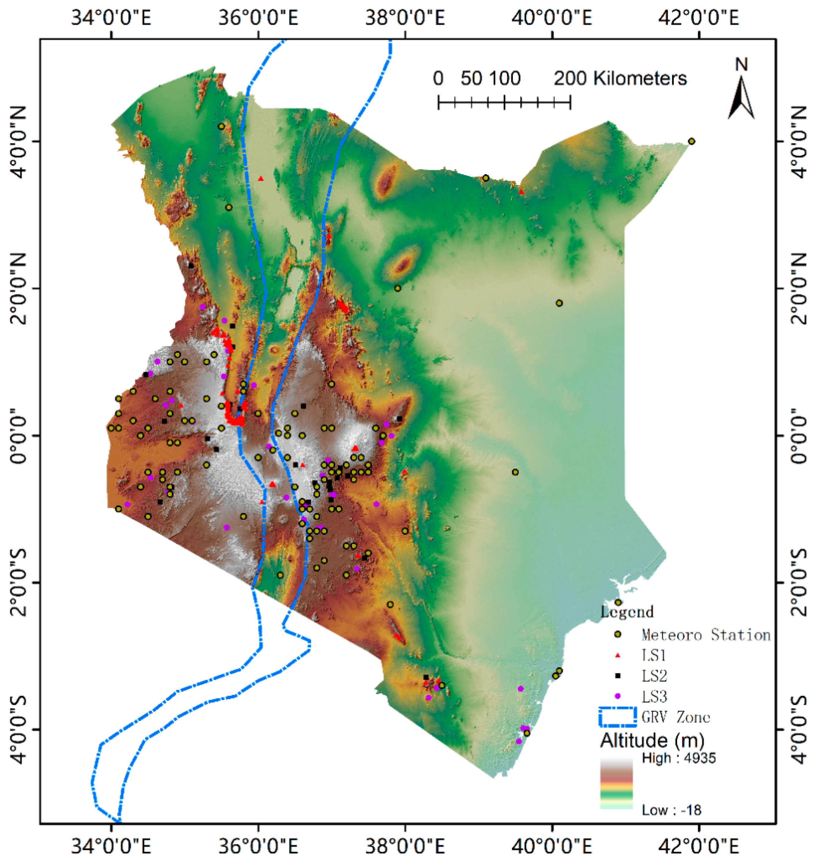
Figure 1. General conditions of Kenya and the spatial distribution of historical landslides in Kenya.
Land 09 00535 g001
Figure 2. Statistics of monthly average precipitation and distribution of landslides in Kenya. Precipitation data was obtained from the Jomo Kenyatta weather station. Since no detailed information of the exact occurring moth of landslides in LS3, only LS1 and LS2 data were included in this figure.
Land 09 00535 g002
Figure 3. List of landslide contribution factors: (a) MAP; (b) altitude; (c) slope; (d) aspect; (e) curvature; (f) TWI; (g) SPI; (h) soil texture; (i) land use; (j) landform.
Land 09 00535 g003
Figure 4. Illustration of the membership function of TFNs.
Land 09 00535 g004
Figure 5. The landslide susceptibility map produced using the TFN-AHP.
Land 09 00535 g005
Figure 6. Area coverage of the five landslide susceptibility levels in Kenya.
Land 09 00535 g006
Figure 7. Area coverage of the five landslide susceptibility levels in each province.
Land 09 00535 g007
Figure 8. Distribution of known landslides in each landslide susceptibility level.
Land 09 00535 g008
Figure 9. ROC curve validation for the obtained landslide susceptibility maps.
Land 09 00535 g009
Figure 10. The landslide susceptibility map produced using the conventional AHP.
Land 09 00535 g010
Table 1. Studies of landslide susceptibility mapping at nation scale.
No.CountryLSM MethodCell Size (m)Landslide Inventory AvailabilityNo. of Causative FactorsSource
1CubaIntegrating SMCE and AHP90No5Abella and Van Westen [21]
2RomaniaHeuristic Weighting100Yes6Bălteanu et al. [22]
3GreeceIntegrating Landslide Relative Frequency and R-mode1000Yes10Sabatakakis et al. [23]
4FranceIntegrating SMCE and Expert Knowledge90Yes3Malet et al. [24]
5GeorgiaSMCE100Yes9Gaprindashvili and Van Westen [25]
6TurkeyHeuristic Weighting500Yes6Okalp and Akgün [26]
7RwandaSMCE30Yes8Nsengiyumva et al. [27]
Table 2. Triangular fuzzy scale used in this study.
Linguistic VariablesIntensity of Conventional AHPReciprocal of IntensityTriangular Fuzzy Number (TFN)Reciprocal of TFN
Equally Important (EQI)11(1,1,2)(1/2,1,1)
Slightly Important (SLI)31/3(2,3,4)(1/4,1/3,1/2)
Moderately Important (MOI)51/5(4,5,6)(1/6,1/5,1/4)
Very Important (VEI)71/7(6,7,8)(1/8,1/7,1/6)
Extremely Important (EXI)91/9(8,9,9)(1/9,1/9,1/8)
Intermediate value21/2(1,2,3)(1/3,1/2,1)
41/4(3,4,5)(1/5,1/4,1/3)
61/6(5,6,7)(1/7,1/6,1/5)
81/8(7,8,9)(1/9,1/8,1/7)
Table 3. Labeling of data according to its predicted label and actual label.
Actual LabelPredicted Lable
PositiveNegative
PositiveTrue Positive(TP)False Negative(FN)
NegativeFalse Positive(FP)True Negative(TN)
Table 4. Pairwise comparison matrix of the LCFs.
LCFLand UseAMPAspectSoil TextureTWISPICurvatureAltitudeLandformSlope
Land use(1,1,1)(1/3,1/2,1/1)(1,2,3)(1/3,1/2,1)(1/3,1/2,1)(1/3,1/2,1)(1/5,1/4,1/3)(1/3,1/2,1)(1/3,1/2,1)(1/5,1/4,1/3)
AMP(1,2,3)(1,1,1)(1,2,3)(2,3,4)(2,3,4)(2,3,4)(1,2,3)(2,3,4)(3,4,5)(2,3,4)
Aspect(1/3,1/2,1)(1/3,1/2,1)(1,1,1)(1/3,1/2,1)(1/3,1/2,1)(1/3,1/2,1)(1/3,1/2,1)(1,2,3)(1/3,1/2,1)(1/4,1/3,1/2)
Soil Texture(1,2,3)(1/4,1/3,1/2)(1,2,3)(1,1,1)(1,2,3)(1,2,3)(1/4,1/3,1/2)(1/5,1/4,1/3)(1,2,3)(1/5,1/4,1/3)
TWI(1,2,3)(1/4,1/3,1/2)(1,2,3)(1/3,1/2,1)(1,1,1)(1,1,2)(1/3,1/2,1)(1,2,3)(1,2,3)(1/5,1/4,1/3)
SPI(1,2,3)(1/4,1/3,1/2)(1,2,3)(1/3,1/2,1)(1/2,1,1)(1,1,1)(1/3,1/2,1)(1/3,1/2,1)(1,2,3)(1/5,1/4,1/3)
Curvature(3,4,5)(1/3,1/2,1)(1,2,3)(2,3,4)(1,2,3)(1,2,3)(1,1,1)(1,2,3)(2,3,4)(1,2,3)
Altitude(1,2,3)(1/4,1/3,1/2)(1/3,1/2,1)(3,4,5)(1/3,1/2,1)(1,2,3)(1/3,1/2,1)(1,1,1)(2,3,4)(1/5,1/4,1/3)
Landform(1,2,3)(1/5,1/4,1/3)(1,2,3)(1/3,1/2,1)(1/3,1/2,1)(1/3,1/2,1)(1/4,1/3,1/2)(1/4,1/3,1/2)(1,1,1)(1/3,1/2,1)
Slope(3,4,5)(1/4,1/3,1/2)(2,3,4)(3,4,5)(3,4,5)(3,4,5)(1/3,1/2,1)(3,4,5)(1,2,3)(1,1,1)
Table 5. The calculation of degree possibility for SiSj and weight of LCFs.
LCFsSi
SLand UseSMAPSAspectSSoil TextureSTWISSPISCurvatureSAltitudeSLandformSSlope
SjSland use--1.00001.00001.00001.00001.00001.00001.00001.00001.0000
SMAP0.1858--0.23010.52370.51750.40540.88360.60870.27941.0000
SAspect0.97531.0000--1.28671.00001.00001.00001.00001.00001.0000
SSoil Texture0.67081.00000.7063--0.97480.89601.00001.00000.76851.0000
STWI0.69151.00000.72741.0270--0.92231.00001.00000.79191.0000
SSPI0.77321.00000.80591.09971.0000--1.00001.00000.87211.0000
SCurvature0.31901.00000.36160.65580.64530.5405--0.74010.41381.0000
SAltitude0.56261.00000.60350.91460.89260.80161.0000--0.66641.0000
SLandform0.90081.00000.92881.21941.00001.00001.00001.0000--1.0000
SSlope0.11460.97960.16370.47730.47230.35050.85850.56740.2155--
min{V(SiSj)}0.11460.97960.16370.47730.47230.35050.85850.56740.21551.0000
Table 6. Calculated weights for the LCFs and their subclasses.
LCFWeightWeights for Subclasses
Altitude0.1091Subclass<5050–200200–500500–10001000–2000>2000
Sub-weight0.060050.1163250.1321930.3327560.2480170.110659
Slope0.1923Subclass0–55–1010–1515–30>30
Sub-weight0.2725760.0718250.1033120.1879740.364313
Aspect0.0315SubclassEastNorthSouthFlatSoutheastNortheastNorthwestSouthwestWest
Sub-weight0.0616930.1489050.1042210.0355640.0646010.1024140.1536850.1309820.197935
Curvature0.1651SubclassConcaveFlatConvex
Sub-weight0.3569560.073030.570014
TWI0.0908Subclass6.8–9.879.88–12.0612.07–14.6814.69–18.7318.74–34.72
Sub-weight0.1936170.1450430.1305910.2516170.279132
SPI0.0674Subclass−2.41–4.61−2.41–4.61−2.41–4.61−2.41–4.61−2.41–4.61
Sub-weight0.1542670.0721070.2366410.217160.319825
Soil Texture0.0918SubclassVery clayedClayedLoamySandyWater
Sub-weight0.3473430.2401270.0642010.195570.152758
Land use0.0220SubclassGrasslandBarren landBushlandWaterbodyPlantationAgricultureTownForrestSwampWoodland
Sub-weight0.1216850.1607430.1364640.0598850.1054350.0985110.0699570.0932530.072470.081596
Landform0.0414SubclassDepressionEscarpmentWaterHighlandHillMountainPlainRidgesValley floorFoot slope
Sub-weight0.1493530.1751070.0221590.0999690.0699480.1626010.0106860.2108270.0383020.061047
AMP0.1884Subclass0–400400–800800–12001200–16001600–20002000–2400>2400
Sub-weight0.1539780.1481630.0386920.0696280.1668770.1980690.224593
Publisher’s Note: MDPI stays neutral with regard to jurisdictional claims in published maps and institutional affiliations.