How Important Are Resistance, Dispersal Ability, Population Density and Mortality in Temporally Dynamic Simulations of Population Connectivity? A Case Study of Tigers in Southeast Asia

Abstract

Development of landscape connectivity and spatial population models is challenging, given the uncertainty of parameters and the sensitivity of models to factors and their interactions over time. Using spatially and temporally explicit simulations, we evaluate the sensitivity of population distribution, abundance and connectivity of tigers in Southeast Asia to variations of resistance surface, dispersal ability, population density and mortality. Utilizing a temporally dynamic cumulative resistant kernel approach, we tested (1) effects and interactions of parameters on predicted population size, distribution and connectivity, and (2) displacement and divergence in scenarios across timesteps. We evaluated the effect of varying levels of factors on simulated population, cumulative resistance kernel extent, and kernel sum across nine timesteps, producing 24,300 simulations. We demonstrate that predicted population, range shifts, and landscape connectivity are highly sensitive to parameter values with significant interactions and relative strength of effects varying by timestep. Dispersal ability, mortality risk and their interaction dominated predictions. Further, population density had intermediate effects, landscape resistance had relatively low impacts, and mitigation of linear barriers (highways) via lowered resistance had little relative effect. Results are relevant to regional, long-term tiger population management, providing insight into potential population growth and range expansion across a landscape of global conservation priority.

1. Introduction

Population dynamics are the result of the interplay between birth, death, immigration and emigration. Classic population models assume well-mixed populations with no spatial structure (e.g., [1,2]). Spatially explicit population models typically have adopted a metapopulation framework [3] in which a network of populations interact through dispersal. However, in many cases, populations are better characterized as gradient systems of differential density, mortality, dispersal and other factors across heterogeneous landscapes [4]. In real landscapes, populations grow, shrink, spread, and contract through space and time in response to spatially varying habitat quality gradients, patterns of mortality risk, and how landscape features drive movement and dispersal. Accounting for temporally dynamic interactions among spatially explicit patterns of habitat quality, mortality rates and dispersal is a deeply challenging task [5,6].

Dispersal, range expansion, population viability, and other processes of research and management interest emerge from complex interactions between a species’ life-history traits, landscape configuration, and anthropogenic influence [7,8,9]. Researchers developing models of population dynamics in complex landscapes face the challenging prospect of capturing these influential factors sufficiently to produce reliable outputs. At a fundamental level, population dynamics are influenced considerably by landscape heterogeneity at multiple scales and ecological patterns affecting biological processes, such as population connectivity. Specifically, connectivity emerges as a function of the ability of organisms to move across the landscape in response to three factors: distribution and density of the source population, resistance of the landscape, and dispersal ability of the organism [10]. Perhaps most important, and usually unaccounted for, spatially-heterogeneous mortality risk can dominate trajectories of population dynamics through space and time [11,12]. To reliably predict population dynamics and connectivity, it is therefore essential to integrate distribution, abundance, resistance, dispersal ability and mortality risk explicitly into integrated spatial models (e.g., [5,6]).

Variation in these parameters may drastically influence results. For example, a number of studies have shown a high degree of sensitivity and complex interactions among factors affecting population size, distribution and connectivity [5,6,9,12,13,14,15]. Empirical data necessary for accurate parameterization of models may be difficult to obtain [16]. Thus, if researchers develop models via a narrowly or vaguely-defined set of parameters, as is often the case [17], they may be limited in their ability to ascertain if model predictions reflect what is likely to occur in reality. In addition, it is essential to understand the relative sensitivity of models to variation in critical parameters, to assess how reliable they are, given parametric uncertainty, and to guide on where empirical or theoretical research should focus to improve the precision of parameter estimates.

There are several key factors in the development of connectivity models used in spatially explicit modeling of population dynamics that merit investigations into their effect. Such models are often highly reliant on resistance surfaces, which define step-wise cost to movement and can aid in determining paths for dispersal, and has received a high degree of focus (e.g., [16]). However, there has been comparatively less attention on investigating the potential effect of non-linear relationships between landscape configuration and cost to movement [9,18]. Importantly, while resistance surfaces may implicitly incorporate mortality as a constraint to movement [19], they may be a poor correlate for elevated mortality risk (e.g., hunting/poaching, road collisions, etc.) during dispersal, that can otherwise drastically affect conclusions on functional connectivity in a landscape [11,20,21]. In reality, mortality risk across landscapes can be highly spatially heterogeneous and models may not explicitly incorporate or investigate its effects [12,22]. Predictions of landscape configuration and connectivity can also be extremely sensitive to species dispersal ability or related parameters dictating movement thresholds [23,24]. This reinforces the need for investigations into model sensitivity to dispersal ability, particularly given that empirical movement data is rarely available to inform model development [16]. Lastly, investigations into the degree to which thresholds of population density or size interact with these and other factors are less common than investigations into the effect of these factors on population metrics [9,25].

Simulation modeling has emerged as a critical investigation tool to understand and predict spatially explicit population dynamics. Simulations can enable researchers to test hypotheses on the effect of varying parameter values on predicted population distributions, abundance and landscape connectivity [5,6,12,15]. However, somewhat neglected has been the use of simulations evaluating temporal dynamics in a spatially explicit framework [26]. Incorporating time-sensitivity and temporal dynamism in analysis enables evaluation of the degree of displacement from initial conditions through time, divergence between scenarios at each timestep, and time-lags in species response to landscape configurations [26].

This study evaluates the degree to which simulations of population and connectivity dynamics in a spatially explicit context are sensitive to the variation of critical parameters. Specifically, we apply a dynamic spatial modeling approach, using cumulative resistance kernels [5,6] and spatially differential mortality risk to test: (1) the strength of effects and interactions of parameters on predicted population size, distribution and connectivity, and (2) the degree of displacement and divergence among scenarios across timesteps. Concurrently, we evaluate the implications of these effects for the regional conservation of an endangered species, the Indochinese tiger (Panthera tigris corbetti). We utilized data from a population of tigers in the Dong Phayayen-Khao Yai forest complex (DPKY) in Eastern Thailand [27]. We consider this to be an ideal candidate species since tigers are wide-ranging, occur within metapopulations shaped considerably through dispersal and landscape configuration, and are a species of notable and urgent conservation concern [28,29]. Tigers have suffered severe range collapse throughout Southeast Asia, likely being extirpated from Cambodia, Laos, and Vietnam [30,31,32]. Our focal landscape of DPKY is likely to be the eastern-most breeding population of tigers in Southeast Asia and may serve as a source population for recolonization of areas in which they were extirpated both within and beyond this landscape. Understanding the population dynamics of this landscape, its degree of connectivity with other potential habitats, and how these factors change over time will be critical for developing long-term management and conservation strategies.

2. Materials and Methods

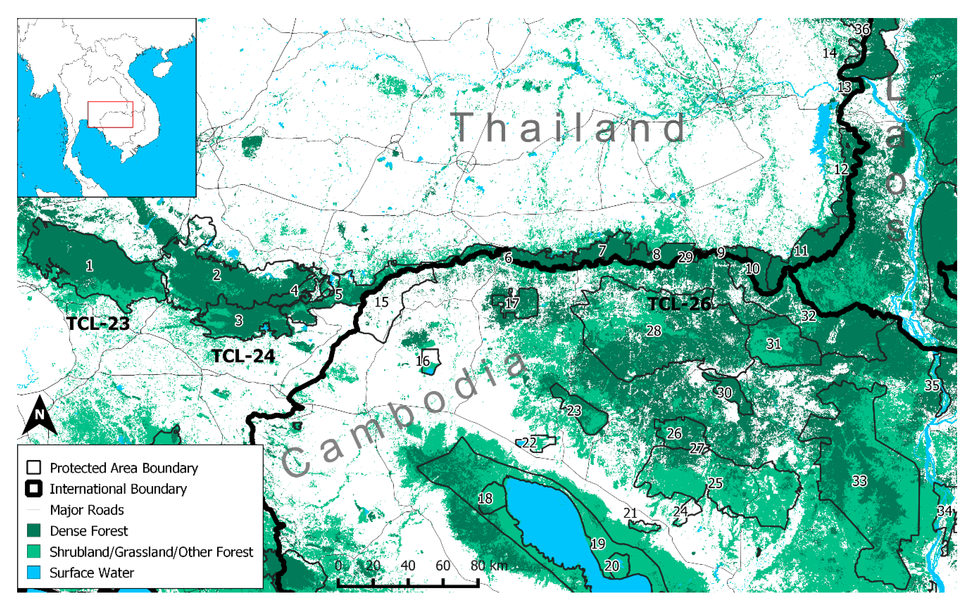
2.1. Study Area

Our study area (Figure 1) contains three tiger conservation landscapes (TCLs; [33]) with notable protected area and forest coverage: the Dong Phayayen-Khao Yai Forest Complex in Eastern Thailand (DPKY; TCLs-23/24), the Phnom-Dong Rak landscape in Eastern Thailand, and the Cambodian Northern Plains (TCL-26) landscape in Northern Cambodia. DPKY is of particular importance, given it currently supports an established breeding population of tigers (TCL-24; [27]) which could potentially disperse to, and re-colonize, the other TCLs in which tigers have been extirpated (TCL-23/26). To account for potential habitat which may facilitate tiger movement between and beyond these protected area complexes, we generated a 45-km buffer from protected area borders in ArcGIS 10.3.1 (Environmental Systems Research Incorporated, ESRI, Redlands, CA, USA, 2011). This distance was selected based on the maximum scale of analysis considered in Reddy et al. [34] in their investigation of landscape-scale gene flow of tigers in central India. This produced a total study area of ~157,920 km², including parts of Thailand, Cambodia, and a small section of southern Lao PDR. The area contains a heterogeneous mix of topography, forest, and anthropogenic land cover. Forest cover configuration in this area varies considerably, from small, relatively isolated patches to large contiguous forest blocks. Much of this forest cover occurs within protected areas, with most land use outside protected areas dominated by agriculture, villages and urban areas.

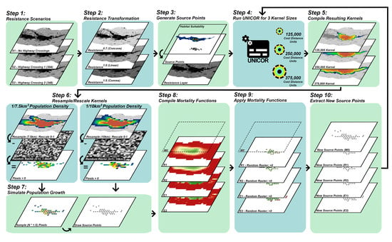
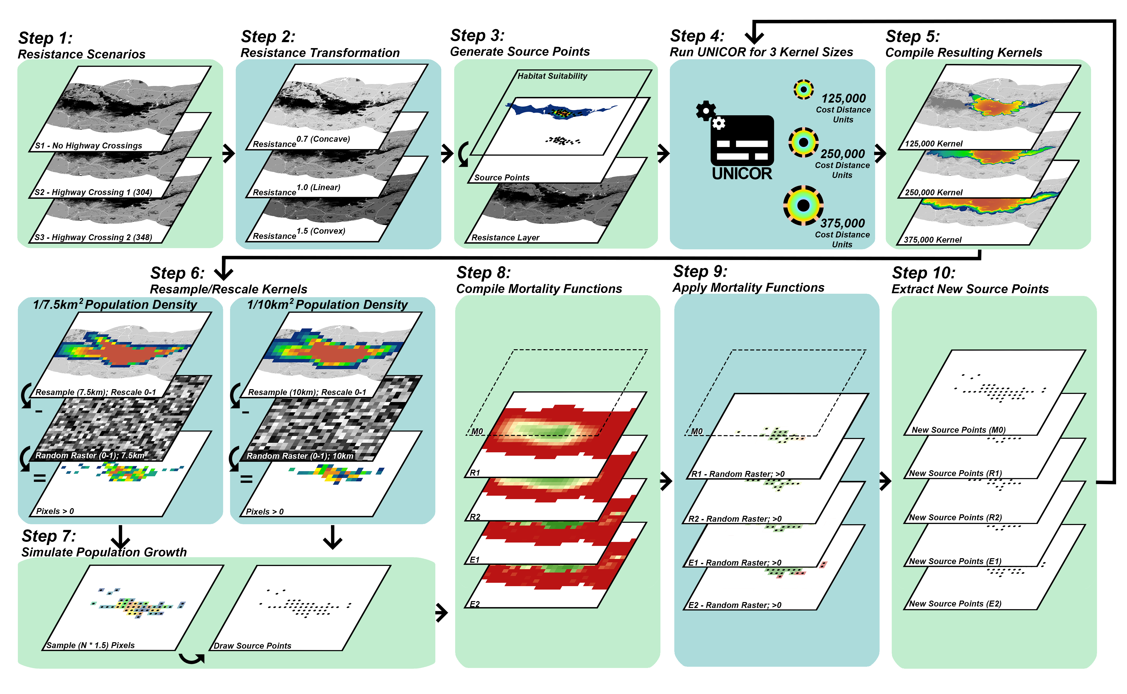
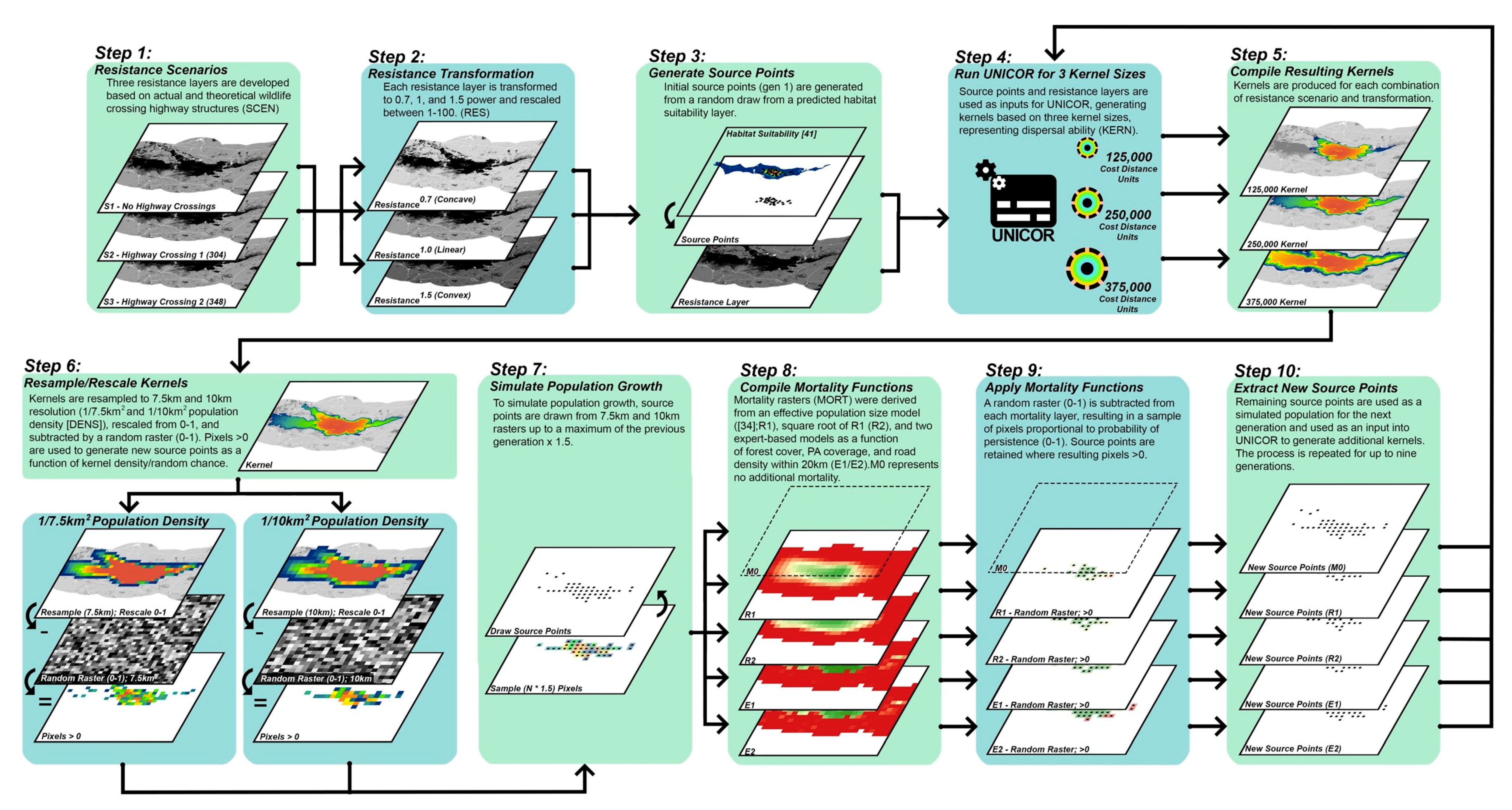
2.2. Landscape Connectivity Simulations

To test the sensitivity of landscape connectivity models, we varied four sets of factors: (1) resistance surface ((i) highway mitigation scenario (SCEN); (ii) resistance transformation (RES)); (2) dispersal ability (KERN); (3) population density (DENS); and (4) mortality function (MORT). Each factor set included several levels to evaluate the influence of adjusting these factors on resulting simulated population (N), cumulative resistance kernel extent (kernext), and kernel sum (kernsum), with kernels generated from the Universal Corridor Network Simulator (UNICOR) v2.0 [38]. A workflow diagram depicting these methods is presented in Figure 2.

2.2.1. Resistance Surfaces

Our approach employs the use of resistance surfaces, a commonly-used foundation for applied connectivity and dispersal modeling [17,39]. In resistance surfaces, pixels in a landscape are assigned values reflecting step-wise cost to individual movement, with low values representing areas of relatively little resistance and high values representing strong resistance. Resistance surfaces assume that landscape-level movement of organisms is dictated by cost of movement and that pixel values in the resistance surface accurately reflect that cost.

Resistance surfaces provide the foundation for connectivity analysis [16], but do not reflect connectivity itself. Specifically, resistance is point specific, but connectivity is path or route specific, governed by source population distribution and density, resistance of the landscape, and dispersal ability of the organism [10]. We employed resistant kernel modeling [40] to simulate the effects of different levels of dispersal ability, mortality, and resistance in predicting the dynamic spread of the tiger population over time. The resistant kernel method is particularly suitable for this application given that it produces a spatial incidence function of the expected rate of movement through each cell in the landscape as a function of source population distribution, resistance and dispersal ability. Thus, this is an ideal method for predicting rates and patterns of dispersal (e.g., [20]) and population spread (e.g., [5,6]).

We tested potential resistance maps generated from Indian connectivity and tiger dispersal models [34,41], an inversed locally-generated habitat suitability model [42], and an expert-derived resistance surface (Supplementary Materials 1). Model predictions varied considerably. Empirical models developed outside our study area either overpredicted resistance of relatively intact lowland forest or overpredicted resistance along potentially important forest ridgelines likely to be used by tigers [43,44]. Further, the inversed locally-generated habitat-suitability model [42] predicted unusually high resistance in areas outside DPKY even in large areas of intact forest cover, potentially owing to third order sampling for the model and a lack of representation of certain habitats occurring outside this landscape. The expert model appeared to reflect patterns of likely tiger presence in DPKY from the empirically-developed habitat-suitability model and predicted low resistance along forested ridgelines and large blocks of forest, while appropriately scaling up resistance in human-dominated areas. Expert-based approaches to parametrize resistance surfaces are often criticized as inaccurately reflecting landscape effects on actual movement [16]. However, given the empirical models tested did not reflect the particular context and limitations of our system and the expert-model reflected behavioral patterns observed in the literature, the expert-derived resistance surface was identified as the most suitable. Additional details can be found in Supplementary Materials 1.

The expert-based approach utilized land cover data from the 2018 SERVIR–Mekong Regional Land Cover Monitoring System (RLCMS; [36]). Land cover was reclassified into five resistance values: Dense forest (1), Scrub forest (20), Agriculture-village matrix (50), Reservoirs/Surface Water (80), and Urban areas (100). Minor and major roads [37] were assigned resistance values of 30 and 100, respectively, where overlapping land-cover values were lower.

Using this resistance layer, we developed three highway mitigation scenarios to test the effect of highway crossing structures (SCEN). Scenarios included: S1—no mitigation of highways (resistance layer as described above); S2—mitigation of local highway route 304 through wildlife crossing structures with lower resistance (20) for pixels representing their present locations; and S3—mitigation of route 304 (S2) and hypothetical mitigation of another local highway, route 348. Further details can be found in Supplementary Materials 1.

To account for resistance uncertainty and evaluate sensitivity to resistance values, we further modified resistance layers to test for three power functions (RES). In addition to the base resistance layer (r10), we also calculated resistance layers to the 0.7 power (r07) and the 1.5 (r15) power which were then rescaled from 1 to 100 and resampled to 250 m resolution. These functions transform the linear shape of the resistance function of landcover into convex (0.7 power) or concave (1.5 power) forms, reflecting different hypotheses about the relative resistance of landcover classes (e.g., [34]).

2.2.2. Population Source Points

To simulate tiger dispersal from DPKY, we derived a set of source points, representing individual animals, which were distributed probabilistically and proportional to tiger habitat suitability (sensu [15,20]). First, we rescaled a multi-scale- and shape-optimized tiger habitat suitability model developed by Ash et al. [41] for DPKY, in which values were proportional to predicted presence on a scale from 0 to 1. Second, we calculated the difference between this layer and a uniform random raster with values ranging from 0 to 1, extracting resulting pixels with positive values as potential source points. Third, we drew a random sample of 30 points from these pixels, representing the upper range of recent population estimates [45]. Source points were generated based on evidence that no tigers currently occur in our study area outside of DPKY [30,32,46].

2.2.3. Dispersal Ability

To evaluate potential dispersal from source points, we utilized UNICOR v2.0 [38] to generate cumulative resistance kernels. These represent the sum of resistance kernels from each source point as a function of total cost distance within the resistance layer and defined kernel width, reflecting predicted density of dispersing individuals for each pixel [13,40]. We tested a range of dispersal abilities (KERN) by applying kernel widths of 125,000 (125 k), 250,000 (250 k), and 375,000 (375 k) cost-distance units (cu) for each scenario (S1, S2, and S3) and resistance transformation (r7, r10, and r15). These kernel widths correspond to potential dispersal distances of 125 km, 250 km, 375 km in ideal habitat (resistance value of 1), respectively. While reliable dispersal data for tigers is rare, tigers are known to disperse within this range of distances [47,48,49]. This enables evaluation of the effect of different dispersal abilities on predicted connectivity (e.g., [13,20]) and population spread [6].

2.2.4. Population Density and Growth

We used a dynamic kernel spread modeling approach first described by Cushman [5] and recently applied in a similar way in Barros et al. [6] which models changes in population distribution across a temporally dynamic framework. Specifically, we modeled population spread across nine discrete timesteps, representing non-overlapping generations. At each timestep, new source points were generated based on kernel layers generated by UNICOR in the previous timestep. To test for the effects of different densities of the tiger population (DENS, e.g., area-specific carrying capacity) these source points were generated at one of two maximum densities. For each factor combination, kernel surfaces were resampled by bilinear interpolation either to 7500 m (7.5 km) or 10,000 m (10 km) resolution. This resulted in two different densities of source points (maximum of 1/56.26 km² or 1/100 km²), reflecting potential differences in simulated territory spacing and carrying capacity of tigers in the study area. These resampled kernel layers were rescaled between 0 and 1, which was then subtracted by a uniform random raster (0–1). This difference raster produced a probabilistic layer for the generation of new source points at both densities for the next timestep, proportional to predicted dispersal density.

To determine the number of source points generated at each timestep and to evaluate simulated population spread, we used a maximum population growth rate of 1.5 per generation timestep (previous generation × 1.5). This assumes half a given population are breeding females with a relatively conservative mean lifetime fecundity of three (see [50,51,52]). These source points were then used as an input to run UNICOR for the next generational timestep. This was repeated for each subsequent timestep (up to 9). In effect, the population (N) and distribution of source points for each timestep and factor combination were based on probabilistic sampling of kernels at one of two densities, a maximum potential population growth rate of 50% per timestep, and random chance.

2.2.5. Mortality

To investigate the potential effect of mortality on the simulated population (MORT), at each timestep we filtered source points based on one of five mortality functions, representing spatially differential probability of survival (pixel values ranging 0 to 1).

Function M0 represents the base scenario described above wherein source points for each timestep were determined by a combination of kernel density, maximum potential population growth rate, and random chance, with no additional modifications.

Functions R1 and R2 were based on a tiger effective population size model from Reddy et al. [34], applied with locally generated spatial layers to predict the potential effective population size of tigers in our study area. The model predicts tiger effective population size as a function of the focal mean of protected area coverage within a 45-km radius, mean forest cover within a 45-km radius, and mean landscape resistance within a 42.5 km radius. In contrast to the resistance model derived from Reddy et al. [34] which defined resistance via specific habitat patterns not reflected in our study landscape, the effective population size model parsimoniously generated predictions broadly applicable to tigers throughout their range (i.e., broad extents of forest cover and protected area presence) [31,53,54,55]. This model produced predictions reflecting reasonable and consistent patterns of high and low potential presence, and by extension, potential survivability across our landscape. This model, rescaled between 0 and 1, was used to predict mortality risk (R1), representing high mortality risk where predicted potential effective population size is low.

To account for uncertainty and investigate the sensitivity of simulations to variation in spatial mortality risk, we calculated the square root of R1, reducing mortality risk in moderate to high suitability areas (R2).

For comparison of approaches and to further test model sensitivity, we also tested two additional expert-based mortality functions with spatially differential probability of mortality (E1 and E2). Evidence suggests that survival probability of dispersing tigers, particularly outside protected areas, can be moderately to extremely low [56,57]. To account for this, we generated a simplified spatially differential mortality risk layer in which survival is a function of available tree cover, protected area coverage, and presence of roads. This layer of spatial probability of survival was capped at 0.8 in protected areas with 100% forest cover and no roads within a 20 km radius, declining in probability as forest cover decrease and road density within 20 km increase, lower by a factor of 10 outside protected areas. To account for uncertainty and to test the sensitivity of results to this mortality function, we also produced a modified expert-derived survivability scenario (E2) following the approach of E1 but modifying the maximum survivability outside protected areas from 10% to 50%. Formulas for these functions are depicted in Supplementary Materials 1.

Mortality functions were applied following the generation of source points for each timestep and parameter combination. At each timestep, mortality layers (values representing low (0) to high (1) probability of survival) were subtracted by a random raster with values from 0 to 1. Source points overlapping with pixels in the difference raster <0 were simulated mortalities and were removed. In effect, mortality-corrected source points were a function of kernel value (expected dispersers arriving at a location in that time step), modeled likelihood of a disperser surviving at that location, and random chance. Resulting source points were then used for the next generation, up to nine generations in total for all combinations of parameters. Additional details on mortality functions and their development are expanded upon in Supplementary Materials 1.

2.3. Evaluation of Simulated Scenarios

Variations in resistance scenarios (SCEN—S1, S2, and S3), non-linear resistance transformation (RES—r07, r10, and r15), dispersal ability (KERN—125 kcu, 250 kcu, and 375 kcu), population density (DENS—7.5 km and 10 km), and mortality function (MORT—M0, R1, R2, E1, and E2) allowed us to simulate a total of 270 tiger population growth and connectivity scenarios across nine generations. To improve the sample size for our evaluation and account for stochastic processes, we ran 10 iterations of each of these scenarios (2700 scenarios with nine generations/timesteps), resulting in a total of 24,300 simulations. Each simulation produced outputs of simulated population size (N), total cumulative kernel extent (kernext), and sum of resistant kernel surface (kernsum, as a total measure of synoptic connectivity).

Simulated population size (N) was defined as the number of source points retained at the end of a given timestep. Kernel extent (kernext) was defined as the count of pixels with values greater than the fiftieth percentile of the distribution of values in the originating cumulative kernel surface at generation 1, for each kernel width (125 kcu, 250 kcu, and 375 kcu). Lastly, kernel sum (kernsum) was calculated as the sum of all pixel values within a cumulative resistance kernel layer. N gives a direct measure of the simulated size of the tiger population, while extent presents the extent of occupied tiger habitat, and kernel sum the total area-weighted density of tigers as a function of population size and connectivity.

To evaluate variation in population and connectivity among simulations, we summarized the frequencies of population trajectories above the baseline population of N = 30, below the baseline, and those in which the population had become extinct (N = 0 by timestep 9). For the purposes of evaluating dispersal from the source population in DPKY, we summarized the frequency of simulations in which source points were generated in Khao Yai National Park (KYNP) in the western section of DPKY, Cambodia, and Laos. We considered these areas successfully colonized if populations persisted to timestep 9.

To test for significant differences between N, kernel extent, and kernel sum across the four investigated factors—resistance surface (SCEN and RES), dispersal ability (KERN), population density (DENS), and mortality function (MORT)—we conducted a factorial analysis of variance (ANOVA), considering differences significant if p < 0.05. To investigate the strength and form of multivariate interactions, we produced time-series maps, surface plots via Matlab (version 18c, MathWorks, Inc., Natick, MA, USA), and multivariate trajectory analysis [26], plotting predicted connectivity values across the nine timesteps/generations for the mean of all replications for each combination of factors. We used Mantel tests [58] to evaluate the effect size and interactions among factors. We evaluated two distance-based response variables, divergence among scenarios, and displacement of scenarios from initial conditions [26]. The Mantel analysis quantifies the effect size (as measured by Mantel r value) of the correlation between the response (divergence or displacement) and whether scenarios had the same or different levels of each factor (SCEN, RES, KERN, DENS, and MORT).

3. Results

Our simulations produced clear and significant differences in simulated population size, kernel extent, and kernel sum trajectories with evidence of strong interactions among factors. These factors drive varying degrees of divergence and displacement from initial states, with implications for patterns of dispersal, colonization, and population persistence. We describe these results in detail below.

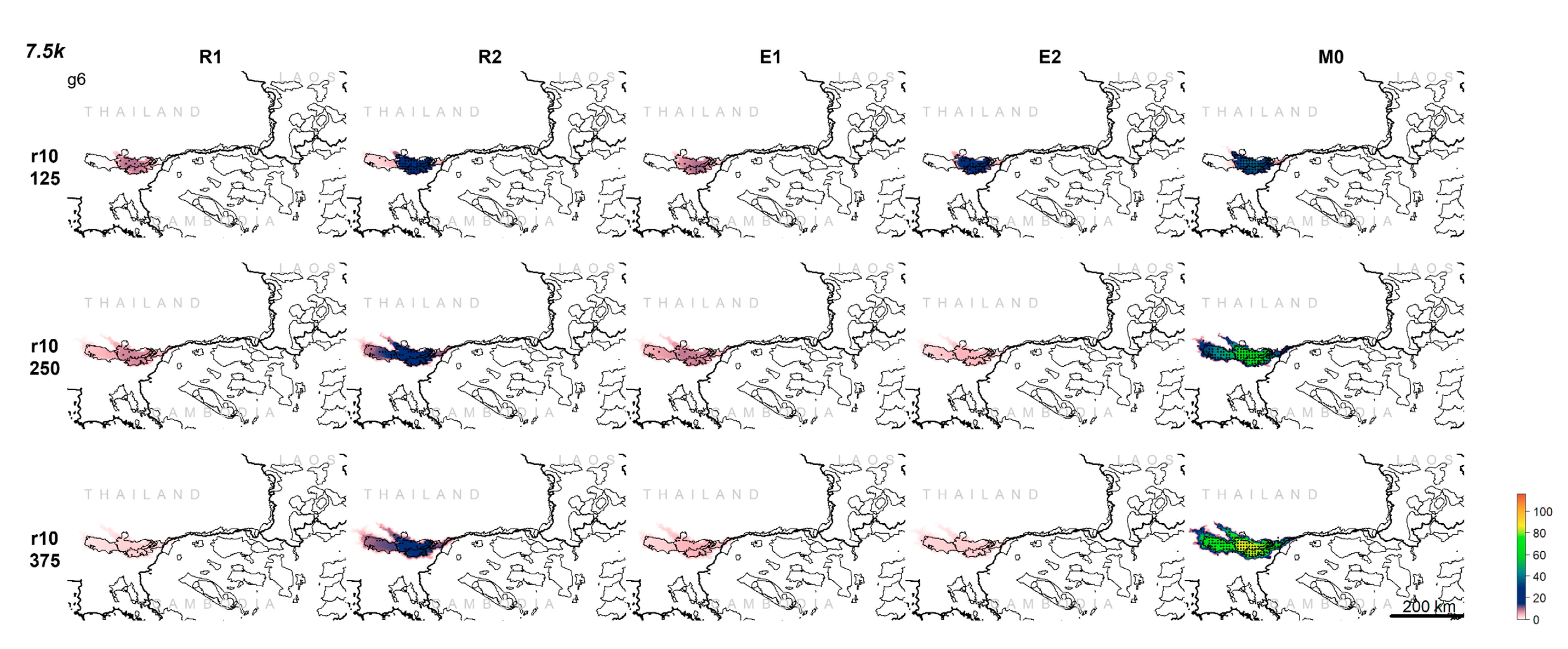
3.1. Population Trajectory and Colonization

The majority of simulations (~73%; 1965), by timestep 9, had population values lower than the baseline (N = 30;

Table 1. Summary of simulation results within factor groups by parameter at timestep 9 out of 2700 simulations. Results are summarized by (a) simulated population (N) at timestep 9 and (b) number of simulations in which source points were generated in Khao Yai National Park (NP), Cambodia, or Laos at timestep 9 (e.g., successful colonization). This reflects a summary of all simulation results specific to each factor group—resistance surface (highway mitigation scenario (SCEN) and resistance transformation, (RES)), dispersal ability (KERN), population density (DENS), and mortality function (MORT)—amalgamating all other factors and parameters. A detailed breakdown of simulation results can be found in Supplementary Materials 2; Tables S1 and S2.

Factor	Parameter	(a)				(b)
		N > 30	N = 30	N = 1 to 30	N = 0	Khao Yai NP	Cambodia	Laos
SCEN	S1	233	7	500	160	455	79	16
	S2	238	11	508	143	498	76	9
	S3	235	11	499	155	472	88	13
DENS	10 km	268	18	812	252	641	99	18
	7.5 km	438	11	695	206	784	144	20
MORT	M0	507	5	28	-	474	235	38
	E1	4	3	363	170	169	1	-
	E2	21	5	393	121	220	1	-
	R1	-	-	373	167	124	-	-
	R2	174	16	350	-	438	6	-
RES	r07	243	17	555	85	438	64	-
	r10	240	5	508	147	473	69	1
	r15	223	7	444	226	514	110	37
KERN	125 kcu	264	17	608	11	371	12	-
	250 kcu	256	10	525	109	609	92	-
	375 kcu	186	2	374	338	445	139	38
	All	706	29	1507	458	1425	243	38

; Supplementary Materials 2, Table S1). In simulations where population values increased, 72% (507) were those with no additional mortality (M0) and higher population density (7.5 km—62% of runs where N > 30). Conversely, population declines were associated primarily with elevated spatially differential mortality functions with little difference among population density, resistance transformation, or dispersal ability. However, the frequency of extinction (population declines to 0 by timestep 9) increased with resistance transformation from concave to convex (19% to 49% of extinctions) and higher dispersal ability (2% of simulated extinctions were with a dispersal ability of 125 kcu, up to 74% with a dispersal ability of 375 kcu).

A large majority of simulations (93%, 2510) resulted in dispersal to KYNP in at least one timestep. However, colonization of KYNP (presence at timestep 9) was considerably lower (53%, 1425; Table 1; Supplementary Materials 2, Table S2). Simulations tended to have a lower frequency of dispersal to KYNP when dispersal ability was lower (79% (712) of simulations with dispersal ability of 125 kcu vs. 100% for 250 kcu and 375 kcu simulations), with much lower rates of successful colonization (41% (371) for 125 kcu, 68% (609) for 250 kcu, and 49% (445) for 375 kcu). Dispersal to this area was also slightly lower for simulations with concave resistance (85% (765) of r07 simulations vs. 95% and 99% for r10 and r15, respectively), and those with larger territory spacing (90% (1217) in simulations with 10 km spacing vs. 96% (1293) with 7.5 km spacing). These trends also hold when considering rates of successful colonization with varying resistance (49% (438) of r07 simulations, 53% (473) of r10 and 57% (514) of r15). Approximately 20% (547) of all simulations resulted in dispersal to areas in Cambodia in at least one timestep, largely attributed to scenarios with no additional mortality (78% (425) instances). Successful colonization of areas in Cambodia was only observed in 9% (243) of simulations, of which 97% (235) were in scenarios with no additional mortality (M0). There was generally a higher rate of dispersal to and colonization of areas in Cambodia as resistance shifted from concave (r07) to convex (r15) forms and as dispersal ability increased (125 kcu to 375 kcu). Only 2% (41) of simulations resulted in dispersal to Laos in any timestep, with only 1% (38) of simulations resulting in colonization. All of these cases were in simulations with no additional mortality (M0) and maximum dispersal ability (375 kcu), with almost all cases when resistance was convex (r15). Dispersal to and colonization of areas outside the source site did not appear substantially affected by highway mitigation scenario (SCEN).

3.2. Analysis of Variance

The factorial analysis of variance of the effects of factors on predicted population size (N), extent of connected population (kernext), and sum of kernel density (kernsum) showed clear and consistent patterns across all three response variables. All main effects, with the exception of highway mitigation scenario (SCEN) and resistance transformation (RES; N at timestep 4)), were very highly significant across timesteps for all three response variables (Supplementary Materials 2, Tables S3–S29). In contrast, SCEN was only significant for timesteps 2–5 for kernsum. Two-way interactions of population density with mortality function (DENS:MORT), mortality function with resistance transformation (MORT:RES), and mortality function with dispersal ability (MORT:KERN) were very highly significant for all timesteps for all three response variables. Two-way interactions of highway mitigation scenario and mortality (SCEN:MORT) were significant for timesteps 2–6 for kernsum and timesteps 5–7 for N. Among three-way interactions, DENS:MORT:KERN was significant in all timesteps across response variables, MORT:RES:KERN was significant for all timesteps and response variables with the exception of two timesteps for N, and DENS:RES:KERN was significant in 75% of time steps for all response variables. The three-way interaction DENS:MORT:RES was significant in 88% of timesteps for N and kernsum, but only 50% of timesteps for kernext. Three-way interactions involving SCEN (SCEN:MORT:RES and SCEN:MORT:KERN) were only significant at timestep 5 for kernsum. None of the other three-way interactions were significant for any timestep for any response variable. The four-way interaction of DENS:MORT:RES:KERN was significant across 75% of timesteps for N, 88% of timesteps for kernsum, and 50% for kernext, and the four-way interaction of SCEN:DENS:MORT:RES was only significant at timestep 3.

The ANOVA results underscore two main outcomes. First, there are strong multivariate interactions, particularly between dispersal ability (KERN), resistance transformation (RES), mortality function (MORT), and territory spacing (DENS). Second, highway mitigation scenario (SCEN) and its interactions did not affect response variables as significantly compared to other factors in our modeling experiment. Given it is difficult to interpret the main effects in the presence of strong interactions, further analysis focused on deconstructing these interactions.

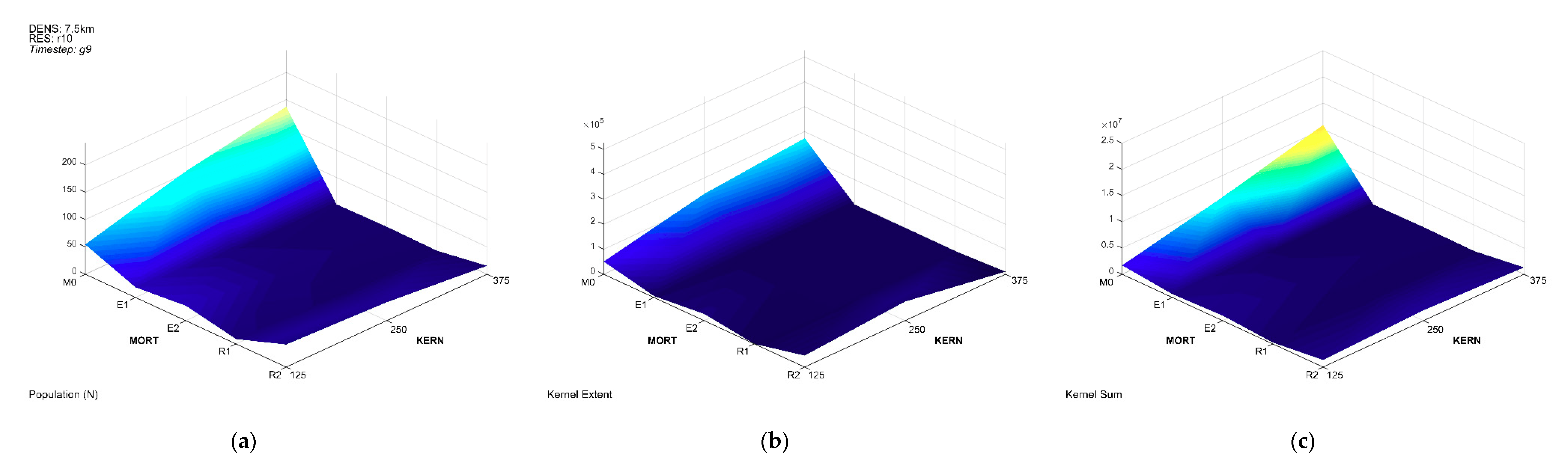
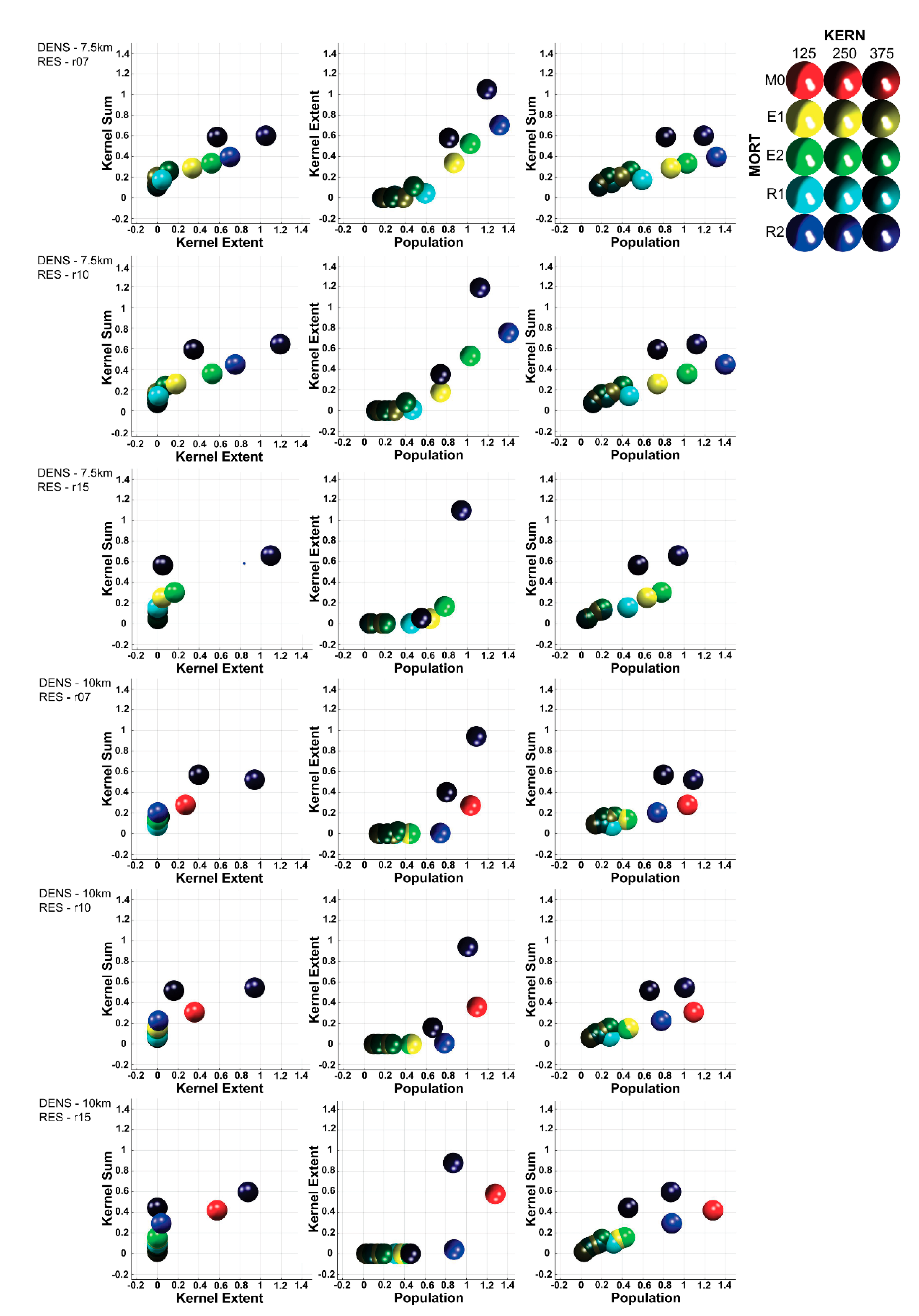
3.3. Multivariate Interactions

Time-series maps (Figure 3; Supplementary Materials 3, Figures S1–S6) and surface plots (Figure 4; Supplementary Materials 3, Figures S7–S12) demonstrated a number of strong interactions between factors. First, mortality function interacts strongly with dispersal ability. In the absence of spatially elevated mortality risk (M0), all three response variables increase dramatically at later timesteps, particularly for simulations with greater dispersal ability and higher potential population density (7.5 km). In contrast, simulations with elevated mortality risk (R1, R2, E1, and E2) show no large increase in any of the three response variables across timesteps, and, in simulations with the highest dispersal ability (375 kcu), populations frequently declined to extinction as a result of dispersal mortality exceeding replacement.

Generally, N and kernsum values increased in simulations with higher maximum potential tiger density (7.5 km), especially in scenarios with higher dispersal and (relatively) lower mortality risk. Kernext increases are greatest in scenarios with low mortality, high dispersal, and lower maximum potential tiger density, as this forces the population to spread more rapidly across a greater extent as available territories fill faster at lower density. The different resistance scenarios interact with mortality, density and dispersal such that N and kernsum variables greatly increase, especially in later timesteps. This is the case when there is low mortality risk, high dispersal, high potential maximum density, and when resistance is convex and does not highly penalize marginal habitat. In this combination of parameters, the rate of population growth is maximized.

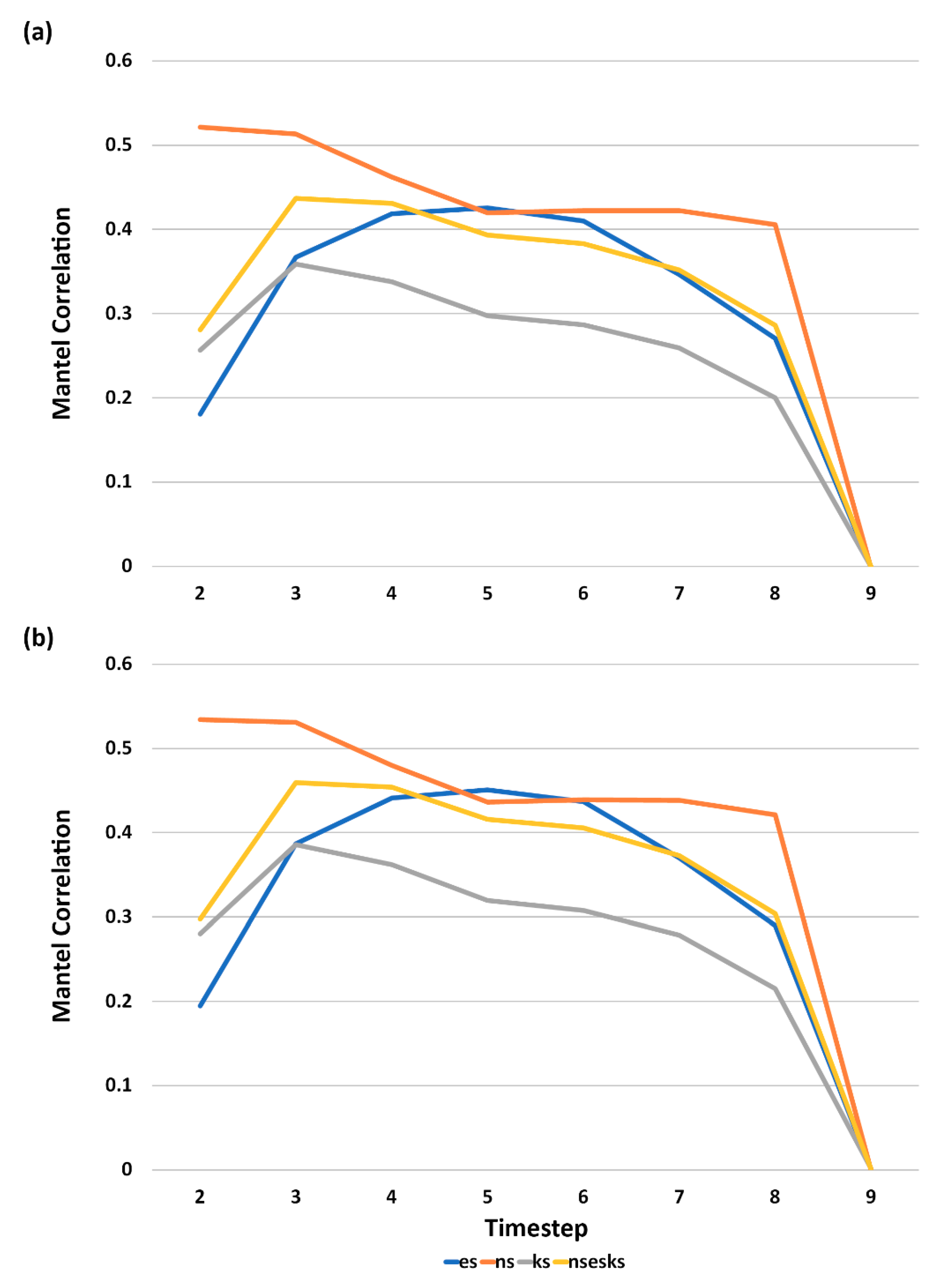
3.4. Multivariate Trajectory Analysis

Multivariate trajectory analysis plots (Figure 5; Supplementary Materials 3, Figures S13–S18), show trajectories over time of simulations corresponding to all combinations of dispersal ability, territory density, resistance transformation, and mortality scenario in a three-dimensional space defined by kernext, kernsum and N. These trajectories show that the major differences are related to mortality risk (MORT) interacting with dispersal ability (KERN), with additional, but lesser effects, from resistance transformation (RES) and population density (DENS). Specifically, most scenarios that have elevated mortality risk as an inverse function of habitat quality do not result in large increases in any of the three connectivity measures (kernext, kernsum or N) over the simulated time frame. In contrast, scenarios in which there is no elevated mortality risk (red spheres in Figure 5) show large increases over time, especially for scenarios in which population density is higher (up to 1/7.5 km²), with substantially lesser effects for different resistance surfaces. Figure 5 shows one view of this three-dimensional space at timestep 6 and readers are encouraged to view the full 3D dynamic visualizations in Supplementary Materials 3.

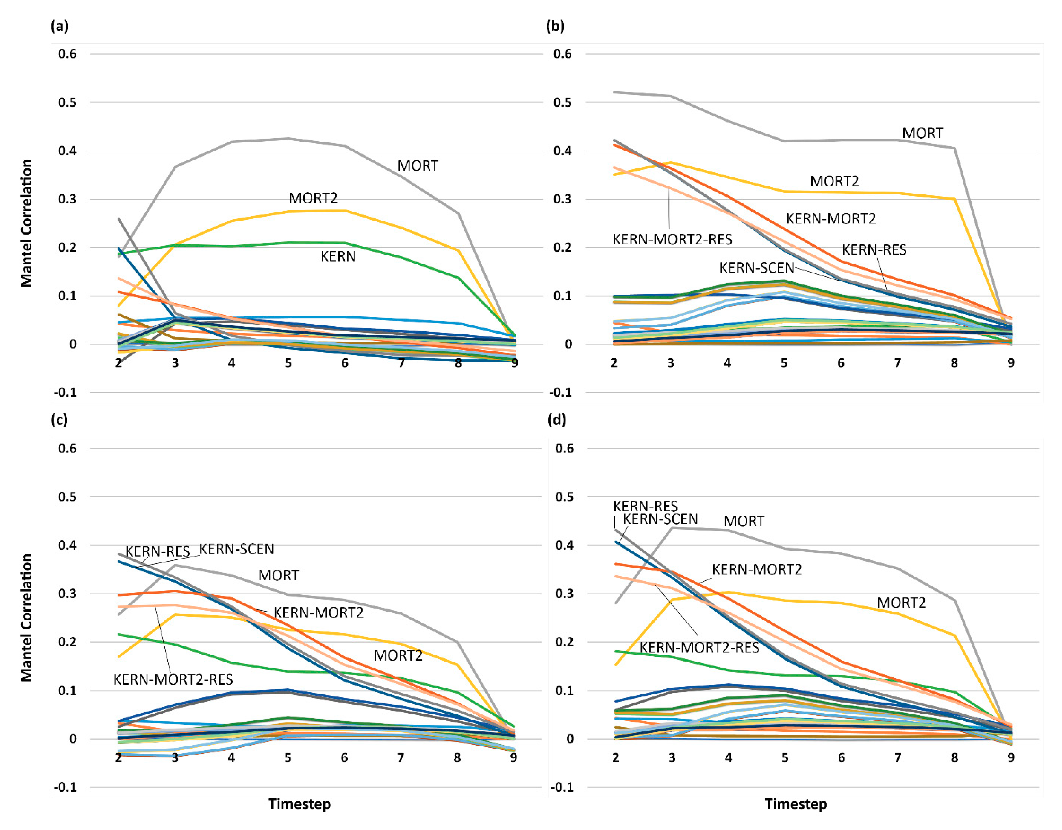
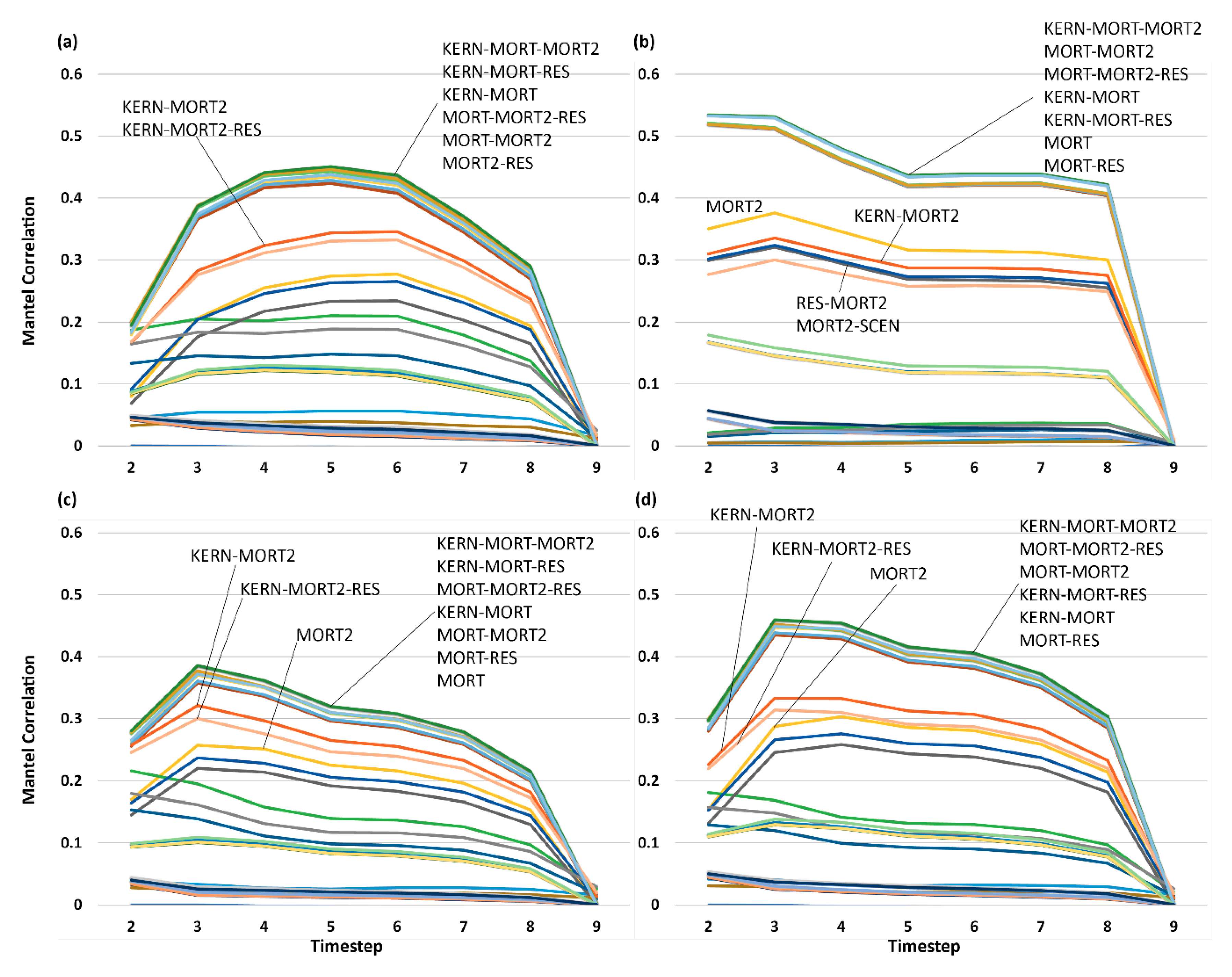
3.5. Analysis of Effect Size and Interactions among Factors Using Mantel Tests

The full table of all Mantel results sorted by effect size is shown in Supplementary Materials 2 (Tables S30–S37) for divergence and displacement, respectively. The main results are most easily presented as line graphs (Figure 6 and Figure 7). For divergence of scenarios from each other over time, mortality function (MORT) had the dominant effect. For each response variable (kernext, kernsum, N and the multivariate combination of these) the mortality model matrix in which all mortality scenarios are coded as 1 and the non-mortality scenarios as 0 was most supported across all timesteps, followed by the ordinal mortality model in which scenarios were ordered from lowest to highest mortality risk (MORT2). Dispersal ability (KERN) and the interaction of dispersal distance and ordinal mortality (KERN-MORT2) had moderate relative effect size, which was nearly equal to mortality in the first few timesteps but dropped to low relative support, comparatively, in later timesteps (Figure 6). For displacement of response variable values from initial condition, there was a different, but even clearer pattern (Figure 7). For all response variables (kernext, kernsum, N and the multivariate combination of these), the interaction between dispersal ability (KERN) and mortality (MORT and MORT2) had the highest Mantel correlation across all timesteps. There was similar support for mortality effects alone (MORT), and mortality interacting with resistance transformation (MORT-RES).

There were consistent relationships in terms of the relative effect size of the correlation between the best model and the four response variables over timesteps (Figure 8). Across all timesteps, the best Mantel model had the largest correlation with predicted N, followed by kernext and the multivariate combination of the three response variables. Kernsum had the lowest correlation with divergence or displacement across all timesteps.

4. Discussion

The ability of models to produce reliable and meaningful predictions of population distribution, abundance and connectivity is governed by the interactive and temporally dynamic effects of several factors such as landscape resistance, population density, dispersal ability, and mortality. Using a spatially and temporally explicit simulation approach, we investigated the impacts of these factors on population connectivity and population size of tigers in Eastern Thailand. Our study demonstrated a high degree of sensitivity of simulated population size, extent and connectivity to parameter values and, in particular, evidence of strong interactions between factors which may drastically affect results. Dispersal ability and spatially differential mortality risk dominated predictions of connectivity and population size, and these factors strongly interacted to affect predictions. While similar dominant effects of dispersal ability on connectivity predictions were previously reported by several studies (e.g., [9,10,20]), less attention has been directed to the effect of spatially differential mortality risk on population size and connectivity [11,12,15].

This is among the first studies to explicitly evaluate the interaction of dispersal ability and mortality on population size, distribution and connectivity in a spatially and temporally explicit dynamic framework. Distribution and density of individuals in the population had intermediate effects on predictions, landscape resistance overall had relatively low impacts on predicted connectivity, and small-scale mitigation of linear barriers had limited measurable impact. Importantly, there was a high degree of variation in the relative importance of factors depending on whether the assessment was based on divergence among scenarios or displacement of scenarios from initial conditions. Furthermore, results differed depending on whether the assessment was based on extent of connected kernel, sum of kernel value, or population size. Our study also documented temporal variation in the relative effects of different factors on connectivity. These results are of particular relevance to the development of connectivity and species dispersal modeling and for conservation planning. We elaborate and discuss each of these main results in the paragraphs that follow.

First, for both displacement (change of a single scenario from initial condition) and divergence (difference between scenarios at a given timestep) of scenarios, we found that spatially heterogeneous mortality risk and dispersal ability dominated predictions of connectivity and population size. Main effects for these factors had very highly significant differences in population and connectivity metrics across all timesteps and exhibited the strongest effects when comparing Mantel correlations. Spatially heterogeneous mortality risk is frequently not accounted for in dispersal and population connectivity modeling studies [12,22], despite evidence that dispersal or hostile matrix-related mortality can exert a considerable influence on species populations and lead to greater vulnerability to demographic stochasticity [59,60,61]. Resistance surfaces, which are widely used, may indirectly account for mortality as a function of a more generalized resistance to dispersal [9,12,15,16,19], though this relationship may be tenuous and lack transparency. Its entanglement with other factors affecting distribution and movement precludes the ability to discern how mortality influences connectivity via realized dispersal, potentially leading to overestimates of the degree of connectivity within a landscape from the perspective of the organism in question [19]. Our results suggest that the application of an additional function of mortality in connectivity modeling can produce highly divergent conclusions on the degree of connectivity within a landscape and trajectory of the population of study. These results are similar to the findings of Kaszta et al. [12] and Kramer-Schadt et al. [11] in which the introduction of mortality risk via infrastructure resulted in isolation and declines of populations of wide-ranging felids that would have otherwise been predicted to be highly connected based on habitat quality and resistance alone.

Similarly, our results were particularly sensitive to dispersal ability, which exerted a relatively disproportionate effect on population and connectivity trajectories. This is consistent with a number of other studies in which predictions of landscape configuration and connectivity were extremely sensitive to parameters associated with dispersal ability or related parameters dictating movement thresholds [23,24]. While some models may be relatively insensitive to dispersal ability [62], this nonetheless underscores the need for particular care in developing these parameters. Ideally, dispersal models should be parameterized with reliable, empirically-derived movement data, though this can be considerably difficult to obtain and are rarely applied in dispersal modeling studies [16,21,28]. This presents a particular challenge to those investigating landscape connectivity where the dispersal ability of target species is poorly understood. Studies in which the latter situation applies may benefit from testing a range of dispersal ability values to account for this uncertainty and potential sensitivity in such parameters.

Second, dispersal ability and mortality risk strongly interacted to affect connectivity predictions, with very high predicted connectivity and population size when dispersal ability is high and mortality risk is low. Importantly, however, when dispersal ability and mortality risk are both high, these factors interacted to produce high mortality rates as dispersing individuals encountered high-risk locations with greater frequency, leading to elevated mortality and declining populations. In these scenarios, overall connectivity and population size remained low and, in some cases, the population declined to extinction even though dispersal ability was high. When mortality risk is high, lower connectivity, due to lower dispersal ability or higher landscape isolation, can produce more viable and larger populations than when dispersal is high [21]. These kinds of interactions were also a key finding of Cushman et al. [9] in which the effects of fragmentation on simulated populations and connectivity became stronger with increasing dispersal ability. Dispersal is a highly costly and risky process [63], and such patterns may emerge when species disperse into hostile, human-dominated matrices. Species with high vagilities are more likely to encounter barriers or sources of mortality during the dispersal process compared to less vagile species [64,65] which may undermine population viability if mortality rates become unsustainably high [11]. In effect, elevated mortality risk in highly fragmented landscapes may result in selection pressure for lower dispersal ability [66]. Gibbs [67] documented greater persistence of organisms in landscapes with low habitat area when dispersal rates were low, a pattern further demonstrated by Cushman et al. [9] through resistant kernel simulation modeling. These patterns are reflective of connectivity being governed by complex interactions of physiological traits, animal behavior, and landscape structure [68]. Given the strong effects of these interactions, it is possible that, without explicitly testing for these in connectivity modeling studies, their effects may remain obfuscated and poorly understood.

Third, we found that mitigating linear barriers, namely major highways, by reducing local resistance in one location, such as through single overpass structures and tunnels, had very limited impact on kernel extent, kernel sum, or population size. There is strong, consistent evidence of the negative effects of roads on connectivity and population persistence [11,22,69,70,71]. Wide-ranging carnivores with long dispersal abilities can be particularly sensitive to fragmentation caused by roads [72,73]. Roads are known to be a source of significant risk for large felids [23,74], potentially leading to isolation of populations when incorporated into movement or genetic models [11,22]. Other factors, particularly mortality and dispersal ability, were more important in our study and dominated patterns of divergence and displacement in our metrics. The literature suggests that one of the critical effects of roads is direct mortality, in some cases, more so compared to their effects as barriers to movement [69]. Such risks were incorporated in our mortality functions which had a large effect, but investigation of finer-scale impacts of roads on individuals was not possible in our study. For studies utilizing cumulative resistance kernels, incorporating the effects of roads by modifying resistance in a small area may result in similar patterns where other factors dominate predictions of connectivity in comparison. The dominating effects of other factors in our study, particularly mortality, reinforces the fact that modeling studies investigating the potential effects of small-scale individual highway mitigation structures must incorporate these factors. Further, costly efforts to mitigate the effects of linear barriers such as highways may be of little benefit if mortality risk and resistance across the landscape as a whole remain high.

Fourth, patterns and degrees of landscape resistance independently had relatively low impacts on predicted connectivity in comparison with dispersal ability and mortality risk. Our results are consistent with evidence from studies utilizing similar methods in which cumulative resistance kernels were found to be relatively insensitive to differences or error in resistance surfaces [13,15,23,40]. Our findings are also aligned with studies in which resistance emerges with weaker effects relative to dispersal ability [9,20,23], which was comparatively stronger in its effect in our study. These results may contribute to evidence that understanding the spatial patterns of mortality risk, dispersal ability of the species and its distribution and abundance in the landscape may be more important than optimal parameterization of resistance surfaces. This is important because a large amount of research has been dedicated to methods of estimating landscape resistance from habitat [16,75], movement [14,76], and genetic [34,76,77] methods. These are often extremely challenging studies that are logistically difficult to implement and highly costly. If landscape resistance is generally of low impact relative to other major factors influencing connectivity and population dynamics, then future investment in research and management application might better be focused on understanding spatial patterns of mortality risk, documenting distribution and abundance of source populations and quantifying movement and dispersal distances with greater precision.

Fifth, distribution and density of individuals in the population had intermediate effects on connectivity predictions, more than resistance, but less than dispersal ability or mortality risk. Similar studies commonly examine how connectivity influences population metrics such as size or density, but there is a dearth of evaluations of how thresholds of population density interact with other factors to influence connectivity [25]. Our results seem consistent with available evidence suggesting models may be sensitive to parameters governing source population size and density (e.g., [10]). Population size, along with dispersal ability were strong factors influencing connectivity in simulations conducted by Cushman et al. [9,10] which found dramatic differences in predicted connectivity and core areas depending on how source locations were modeled (e.g., based on potential vs. actually occupied habitat). This shows that the extant distribution and population size of a focal species has a large influence on the functional connectivity and subsequent changes in population size and connectivity over time. In territorial species, increased density can necessitate dispersal [78]. With larger territory sizes, high-quality habitat may be limited, forcing dispersers to marginal habitat. These patterns are reflected in our study in which higher population density simulations allowed for utilization of available habitat more than those simulating populations at lower density. This resulted in significant differences in population and connectivity metrics.

Sixth, we found variation in the relative importance of factors depending on whether the assessment was based on divergence among scenarios or displacement of scenarios from initial conditions. For divergence between scenarios at the same timestep, mortality risk was predominant, while the interaction between mortality risk and dispersal ability primarily affected displacement of scenarios from initial conditions. Populations are dynamic, and explicitly measuring spatio-temporal dynamism within populations may improve models of ecological change and their interpretation, which may augment the development of management and conservation interventions. Cushman and McGarigal [26] demonstrated this, quantifying important interactions and differences in the magnitude of the effect of timber cutting patterns and intensity on marten habitat over time. Understanding the rate of divergence and displacement in a multivariate response space and quantifying the factors that drive differences in these measures is critical to quantitative and rigorous evaluation of effects of varied and potentially nuanced factors on population size and connectivity in a temporally dynamic context [26].

Seventh, we saw differences in results depending on whether the assessment was based on kernel extent, kernel sum, or population size. Generally, there were higher correlations between factors and population size than with kernel extent or kernel sum, notably with MORT/MORT2 at earlier timesteps. Kernel extent generally had somewhat higher correlations with factors than kernel sum. Both kernel metrics were highly correlated with predicted population size suggesting they may be reliable indicators of effects on population connectivity and viability. These metrics could also, in some cases, be used as a surrogate for population size, which is often harder to estimate or predict. However, population size had a stronger overall relationship than either kernel measures, and, importantly we note that this simulation of population size was built on a kernel model of spread, which makes an objective and independent assessment of the utility of kernel density as a surrogate for population size and density difficult. Nonetheless, past empirical studies [34,62] found strong positive relationships between kernel density predictions and observed species distribution and density. Furthermore, individual-based spatially explicit simulation modeling has shown a strong positive correlation between resistant kernel connectivity predictions and population density [62].

Eighth, we observed considerable temporal variation in the relative effects of different factors on connectivity across our simulation time period. Specifically, we found the impacts of mortality risk peaked at different timesteps for different response metrics. For population size, the correlation was highest in the second timestep, for kernel extent in the fifth, and for kernel sum in the third. This suggests that the effects of different factors on populations and their connectivity are dependent on the context of the population in terms of whether it is expanding from a small initial extent and size or reaching equilibrium with existing landscape conditions. These results reflect evidence of time-dependence in landscape connectivity, an important implication given that connectivity studies often do not account for time in their models [11]. Simulations by Cushman and McGarigal [26] on the effects of forest cutting regimes on marten habitat responses resulted in considerable time-lags in observed effects, occurring decades after anthropogenic disturbance. The potential for these delayed effects has important management implications for a number of species as, in many cases, processes of landscape fragmentation have occurred relatively recently or are ongoing, suggesting their full effects may yet to be realized [15,66]. Being able to discern these effects further reinforces the utility of incorporating timesteps and multivariate trajectory analysis into connectivity modeling.

4.1. Implications for Tiger Management and Conservation

Our study focused primarily on investigating the sensitivity of population and connectivity models to parameterization decisions, using tigers as a case study. Incorporating movement and other empirical data into such models is necessary for generating reliable conclusions [21,28]. The use of such data in connectivity modeling is rare, often resulting from lack of availability, and is a considerable challenge for understudied or endangered species that nonetheless require urgent intervention [16]. In these circumstances, such as for our study population, it is advisable to test a range of parameters to account for this uncertainty and to discern potentially important patterns.

In our study, a number of strong patterns emerged that may have important implications for the conservation of tigers in this landscape. A majority of simulations resulted in dispersal to KYNP, though successful colonization was less frequent. There was a low frequency of dispersal to areas of Cambodia and successful colonization was extremely rare in our study. These cases were primarily simulations with extremely high dispersal ability and convex resistance, and virtually all were with no additional mortality, which is unlikely to be biologically realistic. Mortality was a key factor in our study and would potentially act as a considerable obstacle for long-range dispersal and re-colonization. Further, dispersing tigers tend to have disproportionally higher rates of mortality than established residents in protected areas [57,79]. While male tigers have been known to disperse considerably long distances, female tigers have a tendency for philopatry and shorter dispersal [80,81,82]. This may preclude natural recolonization and recovery in Cambodia and Laos even with low mortality rates.

4.2. Limitations

While our study contributes a number of important insights, simulations are inherently limited, given that models cannot account for the entirety of potential factors that dictate population spread over long time periods, and require empirical validation [16,21]. Our study did not account for dynamic processes of landscape and climate change which may exert considerable influence on our study population over the next several decades. Cambodia, for example, has experienced considerable rates of deforestation and limited protected area security [83,84], which would undermine efforts to support population persistence and maintain broad-scale connectivity. Conversely, we did not test scenarios of habitat restoration which may otherwise augment movement through our study landscape (e.g., [12]). Our framework simplifies processes of population spread that may be further influenced by complex demographic, behavioral, and life-history traits. These may include differential fecundity and variable mortality by age or sex class, or distinguishing between residents and dispersers, which may have drastically different perceptions of the landscape [14]. Further, evidence from other studies suggests a strong relationship between tiger densities and prey abundance, which are likely to influence population persistence and range expansion [51,85]. Ultimately, incorporating these factors would have introduced additional layers of complexity, further entangling confounding factors and making interpretation challenging. While empirical validation is ideal for population connectivity modeling, this is notably challenging for long-term simulation studies such as ours. Nonetheless, given the conservation urgency of many species, it is important to evaluate potential scenarios affecting population size and connectivity before they unfold [15]. We believe our analysis was sufficient for achieving our study objectives, particularly for investigating the sensitivity of models to some of the most central factors that influence connectivity and population spread. Our flexible and powerful framework may prove useful for explicitly testing these additional factors in future studies.

We note that there are a number of potential fine-scale effects that may also influence population dynamics but were only partially addressed by our study. Mortality as an effect is incorporated through mortality functions, though these are introduced at the end of each timestep based on kernel density and random chance. This represents a more explicit process of mortality than is typically inferred via resistance surfaces [16,19]. However, this does not capture finer-scale elevated mortality during dispersal events, such as when simulated individuals cross roads or are poached, which could be a limiting factor in population connectivity [11,22].

Further, mortality in our study was higher outside of protected areas, owing to evidence that dispersal outside these areas is typically associated with a higher risk of mortality [56,57]. However, the effectiveness of protection may vary considerably across formally gazetted protected areas, some of which may lack sufficient deterrents to poaching that may otherwise differentiate these parks from a hostile matrix. We did not test scenarios reflecting high rates of mortality, typical of increased poaching pressure within protected areas or in areas with poor enforcement and high poaching pressure. However, given the strong effect of mortality in our study, this would have likely dramatically increased rates of extinction, reinforcing the importance of reducing mortality at a landscape scale.

Incorporating green infrastructure along highways has been recommended to help mitigate the effects of an expanding network of roads on Southeast Asian wildlife [86]. While we did not document strong effects of individual highway mitigations in our study, we recommend further, dedicated research at finer scales to determine the local effect of existing structures on wildlife in the area. There has been a paucity of studies formally investigating the effect of highway crossing structures on tiger population connectivity. However, studies on other wide-ranging carnivores have documented the use of such structures which could facilitate movement at a landscape scale [87,88,89]. Nonetheless, the types and locations of wildlife crossing structures along linear barriers such as highways should be considered carefully given that use of these structures may vary due to a number of complex factors and by species [90,91]. Purported benefits of wildlife crossing structures included in infrastructure development planning may not sufficiently justify the construction of new roads in areas of wildlife conservation importance. We echo the sentiment of Ash et al. [92] recommending limited development of infrastructure that could fragment habitat or facilitate access in DPKY, such as roads, particularly given the strong effects of mortality in our study.

5. Conclusions

Our study provides a number of insights that may be informative for future applications of spatially explicit modeling in dynamic population and landscape connectivity assessments, particularly for rare or threatened species. This study demonstrates that spatial population and connectivity models can be highly sensitive to model parameters, producing highly divergent patterns of connectivity and population trajectories. Notably, ours is one of the first studies to explicitly evaluate the interaction of dispersal ability and mortality on population size, distribution and connectivity in a spatially explicit dynamic framework. These factors were dominant in our study and we recommend that future studies explicitly account for spatially differential mortality and potential interactions with dispersal ability. Our study also underscores the importance of incorporating a temporally explicit framework into models, given the potential for strong differences in the effect of factors across timesteps that may affect interpretation. Explicitly quantifying patterns of divergence between factors and displacement from initial conditions is crucial for reliably evaluating changes in connectivity over time. In the absence of empirical data to parameterize dispersal and connectivity models more reliably, our approach of evaluating model sensitivity via cumulative resistance kernels is particularly useful to investigate the differential effects of a range of factors. Our study identifies potential population growth and range expansion scenarios for tigers along with key factors relevant to their long-term management across a landscape of global conservation priority.

References

1. Lotka, A.J. The growth of mixed populations: Two species competing for a common food supply. J. Washingt. Acad. Sci. 1932, 22, 461–469. [Google Scholar]
2. Volterra, V. Variations and fluctuations of the number of individuals in animal species living together. ICES J. Mar. Sci. 1928, 3, 3–51. [Google Scholar] [CrossRef]
3. Levins, R. Some mathematical problems in biology. In Extinction; The American Mathematical Society: Providence, RI, USA, 1970; pp. 77–107. [Google Scholar]
4. Cushman, S.A.; H. McRae, B.; McGarigal, K. Basics of Landscape Ecology: An Introduction to Landscapes and Population Processes for Landscape Geneticists. In Landscape Genetics; Wiley Online Books; Balkenhol, N., Cushman, S.A., Storfer, A.T., Waits, L.P., Eds.; John Wiley & Sons, Ltd.: Chichester, UK, 2015; pp. 9–34. ISBN 9781118525258. [Google Scholar]
5. Cushman, S.A. Pushing the envelope in genetic analysis of species invasion. Mol. Ecol. 2015, 24, 259–262. [Google Scholar] [CrossRef]
6. Barros, T.; Carvalho, J.; Fonseca, C.; Cushman, S.A. Assessing the complex relationship between landscape, gene flow, and range expansion of a Mediterranean carnivore. Eur. J. Wildl. Res. 2019, 65, 44. [Google Scholar] [CrossRef]
7. Walters, S. Modeling scale-dependent landscape pattern, dispersal, and connectivity from the perspective of the organism. Landsc. Ecol. 2007, 22, 867–881. [Google Scholar] [CrossRef]
8. Diffendorfer, J.E. Testing Models of Source-Sink Dynamics and Balanced Dispersal. Oikos 1998, 81, 417–433. [Google Scholar] [CrossRef]
9. Cushman, S.A.; Compton, B.W.; McGarigal, K. Habitat Fragmentation Effects Depend on Complex Interactions Between Population Size and Dispersal Ability: Modeling Influences of Roads, Agriculture and Residential Development Across a Range of Life-History Characteristics. In Spatial Complexity, Informatics, and Wildlife Conservation; Cushman, S.A., Huettmann, F., Eds.; Springer: Tokyo, Japan, 2010; pp. 369–385. ISBN 978-4-431-87771-4. [Google Scholar]
10. Cushman, S.A.; Landguth, E.L.; Flather, C.H. Evaluating population connectivity for species of conservation concern in the American Great Plains. Biodivers. Conserv. 2013, 22, 2583–2605. [Google Scholar] [CrossRef] [Green Version]
11. Kramer-Schadt, S.; Revilla, E.; Wiegand, T.; Breitenmoser, U. Fragmented landscapes, road mortality and patch connectivity: Modelling influences on the dispersal of Eurasian lynx. J. Appl. Ecol. 2004, 41, 711–723. [Google Scholar] [CrossRef] [Green Version]
12. Kaszta, Ż.; Cushman, S.A.; Hearn, A.J.; Burnham, D.; Macdonald, E.A.; Goossens, B.; Nathan, S.K.S.S.; Macdonald, D.W. Integrating Sunda clouded leopard (Neofelis diardi) conservation into development and restoration planning in Sabah (Borneo). Biol. Conserv. 2019, 235, 63–76. [Google Scholar] [CrossRef]
13. Cushman, A.S.; Lewis, S.J.; Landguth, L.E. Why Did the Bear Cross the Road? Comparing the Performance of Multiple Resistance Surfaces and Connectivity Modeling Methods. Diversity 2014, 6, 844–854. [Google Scholar] [CrossRef] [Green Version]
14. Elliot, N.; Cushman, S.; Macdonald, D.W.; Loveridge, A. The devil is in the dispersers: The metrics of landscape connectivity change with demography. J. Appl. Ecol. 2014, 51, 1169–1178. [Google Scholar] [CrossRef]
15. Kaszta, Ż.; Cushman, S.A.; Htun, S.; Naing, H.; Burnham, D.; Macdonald, D.W. Simulating the impact of Belt and Road initiative and other major developments in Myanmar on an ambassador felid, the clouded leopard, Neofelis nebulosa. Landsc. Ecol. 2020, 35, 727–746. [Google Scholar] [CrossRef] [Green Version]
16. Zeller, K.A.; McGarigal, K.; Whiteley, A.R. Estimating landscape resistance to movement: A review. Landsc. Ecol. 2012, 27, 777–797. [Google Scholar] [CrossRef]
17. Spear, S.F.; Balkenhol, N.; Fortin, M.J.; McRae, B.H.; Scribner, K. Use of resistance surfaces for landscape genetic studies: Considerations for parameterization and analysis. Mol. Ecol. 2010, 19, 3576–3591. [Google Scholar] [CrossRef] [PubMed]
18. Carroll, K.A.; Hansen, A.J.; Inman, R.M.; Lawrence, R.L.; Hoegh, A.B. Testing landscape resistance layers and modeling connectivity for wolverines in the western United States. Glob. Ecol. Conserv. 2020, 23, e01125. [Google Scholar] [CrossRef]
19. Diniz, M.F.; Cushman, S.A.; Machado, R.B.; De Marco Júnior, P. Landscape connectivity modeling from the perspective of animal dispersal. Landsc. Ecol. 2020, 35, 41–58. [Google Scholar] [CrossRef]
20. Cushman, S.A.; Elliot, N.B.; Macdonald, D.W.; Loveridge, A.J. A multi-scale assessment of population connectivity in African lions (Panthera leo) in response to landscape change. Landsc. Ecol. 2016, 31, 1337–1353. [Google Scholar] [CrossRef]
21. Cushman, S.A. Effects of habitat loss and fragmentation on amphibians: A review and prospectus. Biol. Conserv. 2006, 128, 231–240. [Google Scholar] [CrossRef]
22. Thatte, P.; Joshi, A.; Vaidyanathan, S.; Landguth, E.; Ramakrishnan, U. Maintaining tiger connectivity and minimizing extinction into the next century: Insights from landscape genetics and spatially-explicit simulations. Biol. Conserv. 2018, 218, 181–191. [Google Scholar] [CrossRef]
23. Moqanaki, E.M.; Cushman, S.A. All roads lead to Iran: Predicting landscape connectivity of the last stronghold for the critically endangered Asiatic cheetah. Anim. Conserv. 2017, 20, 29–41. [Google Scholar] [CrossRef] [Green Version]
24. Kanagaraj, R.; Wiegand, T.; Kramer-Schadt, S.; Goyal, S.P. Using individual-based movement models to assess inter-patch connectivity for large carnivores in fragmented landscapes. Biol. Conserv. 2013, 167, 298–309. [Google Scholar] [CrossRef]
25. Carmona, P.; Franco, D. Impact of Dispersal on the Total Population Size, Constancy and Persistence of Two-patch Spatially-separated Populations. Math. Model. Nat. Phenom. 2015, 10, 45–55. [Google Scholar] [CrossRef]
26. Cushman, S.A.; McGarigal, K. Multivariate Landscape Trajectory Analysis. In Temporal Dimensions of Landscape Ecology: Wildlife Responses to Variable Resources; Bissonette, J.A., Storch, I., Eds.; Springer US: Boston, MA, USA, 2007; pp. 119–140. ISBN 978-0-387-45447-4. [Google Scholar]
27. Ash, E.; Kaszta, Ż.; Noochdumrong, A.; Redford, T.; Chanteap, P.; Hallam, C.; Jaroensuk, B.; Raksat, S.; Srinoppawan, K.; Macdonald, D.W.; et al. Opportunity for Thailand’s Forgotten Tigers: Assessment of Indochinese tiger Panthera tigris corbetti and prey from camera-trap surveys in Eastern Thailand. Oryx 2020, 1–8. [Google Scholar] [CrossRef] [Green Version]
28. Vasudev, D.; Nichols, J.D.; Ramakrishnan, U.; Ramesh, K.; Vaidyanathan, S. Assessing Landscape Connectivity for Tigers and Prey Species: Concepts and Practice. In Methods for Monitoring Tiger and Prey Populations; Karanth, K.U., Nichols, J.D., Eds.; Springer: Singapore, 2017; pp. 255–288. ISBN 978-981-10-5436-5. [Google Scholar]
29. Thapa, K.; Wikramanayake, E.; Malla, S.; Acharya, K.P.; Lamichhane, B.R.; Subedi, N.; Pokharel, C.P.; Thapa, G.J.; Dhakal, M.; Bista, A.; et al. Tigers in the Terai: Strong evidence for meta-population dynamics contributing to tiger recovery and conservation in the Terai Arc Landscape. PLoS ONE 2017, 12, e0177548. [Google Scholar] [CrossRef]
30. Rasphone, A.; Kéry, M.; Kamler, J.F.; Macdonald, D.W. Documenting the demise of tiger and leopard, and the status of other carnivores and prey, in Lao PDR’s most prized protected area: Nam Et–Phou Louey. Glob. Ecol. Conserv. 2019, 20, e00766. [Google Scholar] [CrossRef]
31. Goodrich, J.M.; Lynam, A.; Miquelle, D.G.; Wibisono, H.T.; Kawanishi, K.; Pattanavibool, A.; Htun, S.; Tempa, T.; Karki, J.; Jhala, Y.V.; et al. Panthera tigris. IUCN Red List Threat. Species 2015: e.T15955A50659951. 2015. Available online: https://www.iucnredlist.org/species/15955/50659951 (accessed on 26 October 2020).
32. Gray, T.N.E.; Crouthers, R.; Ramesh, K.; Vattakaven, J.; Borah, J.; Pasha, M.K.S.; Lim, T.; Phan, C.; Singh, R.; Long, B.; et al. A framework for assessing readiness for tiger Panthera tigris reintroduction: A case study from eastern Cambodia. Biodivers. Conserv. 2017, 26, 2383–2399. [Google Scholar] [CrossRef]
33. Sanderson, E.; Forrest, J.; Loucks, C.; Ginsberg, J.; Dinerstein, E.; Seidensticker, J.; Leimgruber, P.; Songer, M.; Heydlauff, A.; O’Brien, T.; et al. Setting Priorities for the Conservation and Recovery of Wild Tigers: 2005–2015—The Technical Assessment; WCS, WWF, Smithsonian, and NFWF-STF: New York, NY, USA; Washington, DC, USA, 2006. [Google Scholar]
34. Reddy, P.A.; Cushman, S.A.; Srivastava, A.; Sarkar, M.S.; Shivaji, S. Tiger abundance and gene flow in Central India are driven by disparate combinations of topography and land cover. Divers. Distrib. 2017, 23, 863–874. [Google Scholar] [CrossRef]
35. UNEP-WCMC; IUCN Protected Planet. The World Database on Protected Areas (WDPA). Cambridge, UK. Available online: www.protectedplanet.net (accessed on 15 July 2019).
36. SERVIR-Mekong. SERVIR–Mekong Regional Land Cover Monitoring System (RLCMS); SERVIR-Mekong/USAID/NASA/ADPC/ICIMOD; Asian Disaster Preparedness Center (ADPC): Bangkok, Thailand, 2018. [Google Scholar]
37. OpenStreetMap OpenStreetMap. Available online: www.openstreetmap.org (accessed on 10 June 2019).
38. Landguth, E.L.; Hand, B.K.; Glassy, J.; Cushman, S.A.; Sawaya, M.A. UNICOR: A species connectivity and corridor network simulator. Ecography 2012, 35, 9–14. [Google Scholar] [CrossRef]
39. Graves, T.; Chandler, R.B.; Royle, J.A.; Beier, P.; Kendall, K.C. Estimating landscape resistance to dispersal. Landsc. Ecol. 2014, 29, 1201–1211. [Google Scholar] [CrossRef]
40. Compton, B.W.; McGarigal, K.; Cushman, S.A.; Gamble, L.R. A resistant-kernel model of connectivity for amphibians that breed in vernal pools. Conserv. Biol. 2007, 21, 788–799. [Google Scholar] [CrossRef]
41. Ash, E.; Macdonald, D.W.; Cushman, S.A.; Noochdumrong, A.; Redford, T.; Kaszta, Ż. Optimization of spatial scale, but not functional shape, affects the performance of habitat suitability models: A case study of tigers (Panthera tigris) in Thailand. Landsc. Ecol. in press.
42. Krishnamurthy, R.; Cushman, S.A.; Sarkar, M.S.; Malviya, M.; Naveen, M.; Johnson, J.A.; Sen, S. Multi-scale prediction of landscape resistance for tiger dispersal in central India. Landsc. Ecol. 2016, 31, 1355–1368. [Google Scholar] [CrossRef]
43. Karanth, K.U. Estimating tiger Panthera tigris populations from camera-trap data using capture-recapture models. Biol. Conserv. 1995, 71, 333–338. [Google Scholar] [CrossRef]
44. Karanth, K.U.; Nichols, J.D. Estimation of tiger densities in India using photographic captures and recaptures. Ecology 1998, 79, 2852–2862. [Google Scholar] [CrossRef]
45. Ash, E.; Hallam, C.; Chanteap, P.; Kaszta, Ż.; Macdonald, D.W.; Rojanachinda, W.; Redford, T.; Harihar, A. Estimating the density of a globally important tiger (Panthera tigris) population: Using simulations to evaluate survey design in Eastern Thailand. Biol. Conserv. 2020, 241, 108349. [Google Scholar] [CrossRef]
46. Lynam, A.; Nowell, K. Panthera tigris ssp. corbetti. IUCN Red List Threat. Species 2011: e.T136853A4346984. 2011. Available online: https://www.iucnredlist.org/species/136853/4346984 (accessed on 26 October 2020).
47. Joshi, A.R.; Dinerstein, E.; Wikramanayake, E.; Anderson, M.L.; Olson, D.; Jones, B.S.; Seidensticker, J.; Lumpkin, S.; Hansen, M.C.; Sizer, N.C.; et al. Tracking changes and preventing loss in critical tiger habitat. Sci. Adv. 2016, 2, e1501675. [Google Scholar] [CrossRef] [Green Version]
48. Sarkar, M.S.; Ramesh, K.; Johnson, J.A.; Sen, S.; Nigam, P.; Gupta, S.K.; Murthy, R.S.; Saha, G.K. Movement and home range characteristics of reintroduced tiger (Panthera tigris) population in Panna Tiger Reserve, central India. Eur. J. Wildl. Res. 2016, 62, 537–547. [Google Scholar] [CrossRef]
49. Sunquist, M. What is a Tiger? Ecology and Behavior. In Tigers of the World, 2nd ed.; Tilson, R., Nyhus, P., Eds.; Elsevier: New York, NY, USA, 2010; pp. 19–34. [Google Scholar]
50. Smith, J.L.D.; McDougal, C. The Contribution of Variance in Lifetime Reproduction to Effective Population Size in Tigers. Conserv. Biol. 1991, 5, 484–490. [Google Scholar] [CrossRef]
51. Karanth, K.U.; Stith, B.M. Prey depletion as a critical determinant of tiger population viability. In Riding the Tiger: Tiger Conservation in Human-Dominated Landscapes; Seidensticker, J., Jackson, P., Christie, S., Eds.; Cambridge University Press: Cambridge, UK, 1999; pp. 100–113. ISBN 0521648351. [Google Scholar]
52. Linkie, M.; Chapron, G.; Martyr, D.J.; Holden, J.; Leader-Williams, N. Assessing the viability of tiger subpopulations in a fragmented landscape. J. Appl. Ecol. 2006, 43, 576–586. [Google Scholar] [CrossRef]
53. Walston, J.; Robinson, J.G.; Bennett, E.L.; Breitenmoser, U.; da Fonseca, G.A.B.; Goodrich, J.; Gumal, M.; Hunter, L.; Johnson, A.; Ullas Karanth, K.; et al. Bringing the tiger back from the brink-the six percent solution. PloS Biol. 2010, 8, e1000485. [Google Scholar] [CrossRef] [Green Version]
54. Sunarto, S.; Kelly, M.J.; Parakkasi, K.; Klenzendorf, S.; Septayuda, E.; Kurniawan, H. Tigers need cover: Multi-scale occupancy study of the big cat in Sumatran forest and plantation landscapes. PLoS ONE 2012, 7, e30859. [Google Scholar] [CrossRef] [Green Version]
55. Kafley, H.; Gompper, M.E.; Sharma, M.; Lamichane, B.R.; Maharjan, R. Tigers (Panthera tigris) respond to fine spatial-scale habitat factors: Occupancy-based habitat association of tigers in Chitwan National Park, Nepal. Wildl. Res. 2016, 43, 398. [Google Scholar] [CrossRef]
56. Smith, J.L.D. The Role of Dispersal in Structuring the Chitwan Tiger Population. Behaviour 1993, 124, 165–195. [Google Scholar] [CrossRef]
57. Goodrich, J.M.; Kerley, L.L.; Smirnov, E.N.; Miquelle, D.G.; McDonald, L.; Quigley, H.B.; Hornocker, M.G.; McDonald, T. Survival rates and causes of mortality of Amur tigers on and near the Sikhote-Alin Biosphere Zapovednik. J. Zool. 2008, 276, 323–329. [Google Scholar] [CrossRef]
58. Mantel, N. The Detection of Disease Clustering and a Generalized Regression Approach. Cancer Res. 1967, 27, 209–220. [Google Scholar]
59. Carroll, C.; Miquelle, D.G. Spatial viability analysis of Amur tiger Panthera tigris altaica in the Russian Far East: The role of protected areas and landscape matrix in population persistence. J. Appl. Ecol. 2006, 43, 1056–1068. [Google Scholar] [CrossRef]
60. Thapa, T.B. Human caused mortality in the leopard (Panthera pardus) population of Nepal. J. Inst. Sci. Technol. 2014, 19, 150–155. [Google Scholar] [CrossRef] [Green Version]
61. Naude, V.N.; Balme, G.A.; O’Riain, J.; Hunter, L.T.B.; Fattebert, J.; Dickerson, T.; Bishop, J.M. Unsustainable anthropogenic mortality disrupts natal dispersal and promotes inbreeding in leopards. Ecol. Evol. 2020, 10, 3605–3619. [Google Scholar] [CrossRef]
62. Puyravaud, J.P.; Cushman, S.A.; Davidar, P.; Madappa, D. Predicting landscape connectivity for the Asian elephant in its largest remaining subpopulation. Anim. Conserv. 2017, 20, 225–234. [Google Scholar] [CrossRef]
63. Bonte, D.; Van Dyck, H.; Bullock, J.M.; Coulon, A.; Delgado, M.; Gibbs, M.; Lehouck, V.; Matthysen, E.; Mustin, K.; Saastamoinen, M.; et al. Costs of dispersal. Biol. Rev. 2012, 87, 290–312. [Google Scholar] [CrossRef]
64. Carr, L.W.; Fahrig, L. Effect of Road Traffic on Two Amphibian Species of Differing Vagility. Conserv. Biol. 2001, 15, 1071–1078. [Google Scholar] [CrossRef]
65. Carr, L.W.; Fahrig, L.; Pope, S.E. Impacts of Landscape Transformation by Roads. In Applying Landscape Ecology in Biological Conservation; Gutzwiller, K.J., Ed.; Springer: New York, NY, USA, 2002; pp. 225–243. ISBN 978-1-4613-0059-5. [Google Scholar]
66. Ewers, R.M.; Didham, R.K. Confounding factors in the detection of species responses to habitat fragmentation. Biol. Rev. 2006, 81, 117–142. [Google Scholar] [CrossRef]
67. Gibbs, J.P. Amphibian Movements in Response to Forest Edges, Roads, and Streambeds in Southern New England. J. Wildl. Manag. 1998, 62, 584–589. [Google Scholar] [CrossRef]
68. Goodwin, B.J.; Fahrig, L. How does landscape structure influence landscape connectivity? Oikos 2002, 99, 552–570. [Google Scholar] [CrossRef] [Green Version]
69. Jackson, N.D.; Fahrig, L. Relative effects of road mortality and decreased connectivity on population genetic diversity. Biol. Conserv. 2011, 144, 3143–3148. [Google Scholar] [CrossRef]
70. Kerley, L.I.; Goodrich, J.M.; Miquelle, D.G.; Smirnov, E.N.; Quigley, H.B.; Hornocker, M.G. Effects of Roads and Human Disturbance on Amur Tigers. Conserv. Biol. 2002, 16, 97–108. [Google Scholar] [CrossRef] [Green Version]
71. Coffin, A.W. From roadkill to road ecology: A review of the ecological effects of roads. J. Transp. Geogr. 2007, 15, 396–406. [Google Scholar] [CrossRef]
72. Trombulak, S.C.; Frissell, C.A. Review of Ecological Effects of Roads on Terrestrial and Aquatic Communities. Conserv. Biol. 2000, 14, 18–30. [Google Scholar] [CrossRef]
73. Carroll, C.; Noss, R.F.; Paquet, P.C. Carnivores as focal species for conservation planning in the Rocky Mountain region. Ecol. Appl. 2001, 11, 961–980. [Google Scholar] [CrossRef]
74. Schwab, A.C.; Zandbergen, P.A. Vehicle-related mortality and road crossing behavior of the Florida panther. Appl. Geogr. 2011, 31, 859–870. [Google Scholar] [CrossRef]
75. Keeley, A.T.H.; Beier, P.; Gagnon, J.W. Estimating landscape resistance from habitat suitability: Effects of data source and nonlinearities. Landsc. Ecol. 2016, 31, 2151–2162. [Google Scholar] [CrossRef]
76. Zeller, K.A.; Vickers, T.W.; Ernest, H.B.; Boyce, W.M. Multi-level, multi-scale resource selection functions and resistance surfaces for conservation planning: Pumas as a case study. PLoS ONE 2017, 12, e0179570. [Google Scholar] [CrossRef]
77. Winiarski, K.J.; Peterman, W.E.; Whiteley, A.R.; McGarigal, K. Multiscale resistant kernel surfaces derived from inferred gene flow: An application with vernal pool breeding salamanders. Mol. Ecol. Resour. 2020, 20, 97–113. [Google Scholar] [CrossRef] [PubMed]
78. Matthysen, E. Density-dependent dispersal in birds and mammals. Ecography 2005, 28, 403–416. [Google Scholar] [CrossRef]
79. Gurung, B.; Smith, J.L.D.; McDougal, C.; Karki, J.B. Tiger Human Conflicts: Investigating Ecological and Sociological Issues of Tiger Conservation in the Buffer Zone of Chitwan National Park, Nepal; WWF-Nepal Program: Kathmandu, Nepal, 2006. [Google Scholar]
80. Gour, D.S.; Bhagavatula, J.; Bhavanishankar, M.; Reddy, P.A.; Gupta, J.A.; Sarkar, M.S.; Hussain, S.M.; Harika, S.; Gulia, R.; Shivaji, S. Philopatry and Dispersal Patterns in Tiger (Panthera tigris). PLoS ONE 2013, 8, e66956. [Google Scholar] [CrossRef] [PubMed] [Green Version]
81. Singh, R.; Qureshi, Q.; Sankar, K.; Krausman, P.R.; Goyal, S.P. Use of camera traps to determine dispersal of tigers in semi-arid landscape, western India. J. Arid Environ. 2013, 98, 105–108. [Google Scholar] [CrossRef]
82. Sunquist, M.; Karanth, U.K.; Sunquist, F. Ecology, behaviour and resilience of the tiger and its conservation needs. In Riding the Tiger: Tiger Conservation in Human-Dominated Landscapes; Seidensticker, J., Jackson, P., Christie, S., Eds.; Cambridge University Press: Cambridge, UK, 1999; pp. 5–18. [Google Scholar]
83. Lohani, S.; Dilts, T.E.; Weisberg, P.J.; Null, S.E.; Hogan, Z.S. Rapidly Accelerating Deforestation in Cambodia’s Mekong River Basin: A Comparative Analysis of Spatial Patterns and Drivers. Water 2020, 12, 2191. [Google Scholar] [CrossRef]
84. Rostro-García, S.; Kamler, J.F.; Ash, E.; Clements, G.R.; Gibson, L.; Lynam, A.J.; McEwing, R.; Naing, H.; Paglia, S. Endangered leopards: Range collapse of the Indochinese leopard (Panthera pardus delacouri) in Southeast Asia. Biol. Conserv. 2016, 201, 293–300. [Google Scholar] [CrossRef]
85. Karanth, K.U.; Nichols, J.D.; Kumar, N.S.; Link, W.A.; Hines, J.E. Tigers and their prey: Predicting carnivore densities from prey abundance. Proc. Natl. Acad. Sci. USA 2004, 101, 4854–4858. [Google Scholar] [CrossRef] [Green Version]
86. Clements, G.R.; Lynam, A.J.; Gaveau, D.; Yap, W.L.; Lhota, S.; Goosem, M.; Laurance, S.; Laurance, W.F. Where and how are roads endangering mammals in Southeast Asia’s forests? PLoS ONE 2014, 9, e115376. [Google Scholar] [CrossRef] [Green Version]
87. González-Gallina, A.; Hidalgo-Mihart, M.G.; Castelazo-Calva, V. Conservation implications for jaguars and other neotropical mammals using highway underpasses. PLoS ONE 2018, 13, e0206614. [Google Scholar] [CrossRef] [Green Version]
88. Ford, A.T.; Barrueto, M.; Clevenger, A.P. Road mitigation is a demographic filter for grizzly bears. Wildl. Soc. Bull. 2017, 41, 712–719. [Google Scholar] [CrossRef]
89. Gloyne, C.C.; Clevenger, A.P. Cougar Puma concolor use of wildlife crossing structures on the Trans-Canada highway in Banff National Park, Alberta. Wildl. Biol. 2001, 7, 117–124. [Google Scholar] [CrossRef]
90. Clevenger, A.P.; Waltho, N. Factors Influencing the Effectiveness of Wildlife Underpasses in Banff National Park, Alberta, Canada. Conserv. Biol. 2000, 14, 47–56. [Google Scholar] [CrossRef]
91. Caldwell, M.R.; Klip, J.M.K. Wildlife Interactions within Highway Underpasses. J. Wildl. Manag. 2020, 84, 227–236. [Google Scholar] [CrossRef]
92. Ash, E.; Kaszta, Ż.; Redford, T.; Noochdumrong, A.; Macdonald, D.W. Environmental factors, human presence, and prey interact to explain patterns of tiger presence in Eastern Thailand. Anim. Conserv. 2020. [Google Scholar] [CrossRef]
Figure 1. Study area for connectivity analysis. Protected areas were generated from UNEP-WCMC and IUCN [35]; a full listing of names can be found in Supplementary Materials 1. Forest cover was generated from 2018 SERVIR–Mekong Regional Land Cover Monitoring System (RLCMS; [36]) reclassed into dense forest (including Forest, Evergreen Forest, Flooded Forest, and Mixed Forest), and Shrubland/Grassland/Other Forest (including Shrubland, Grassland, Wetlands and Orchard/Plantation). Major roads were derived from OpenStreetMap [37]. The eastern section (TCL-24) of the Dong Phayayen-Khao Yai forest complex (2–5) acts as the source site for our simulations.
Land 09 00415 g001
Figure 2. Diagram depicting methods workflow, including development of highway crossing resistance scenarios (SCEN), resistance transformation (RES), adjusting dispersal ability (KERN), adjusting population density (DENS), and developing and applying mortality functions (MORT). Ash et al. [41]; Reddy et al. [34].
Land 09 00415 g002
Figure 3. Sample maps demonstrating divergence in cumulative resistance kernels and populations between combinations of mortality function (MORT—R1, R2, E1, E2, and M0) and dispersal ability (KERN—125 kcu, 250 kcu, and 375 kcu) at timestep 6, holding highway mitigation scenario (SCEN—S3), territory spacing (DENS—7.5 km), and resistance transformation (RES—r10) constant. Values reflect the expected cumulative density of dispersing individuals from each source point. Additional maps and timestep animations can be found in Supplementary Materials 3, Tables S1–S6.
Land 09 00415 g003
Figure 4. Surface plots showing variation in predicted (a) population size (N), (b) kernel extent, and (c) sum of kernel value for the 15 combinations of dispersal ability (KERN—3 levels) and mortality risk (MORT—5 levels) for resistance transformation 1.0 (RES—r10) and maximum density 1/7.5 km2 (DENS—7.5 km) at timestep 9. The figure shows a strong interaction between dispersal ability and mortality risk, with the predicted values of all three variables remaining low for all scenarios involving elevated mortality risk, across all dispersal abilities, while all three variables increase linearly with dispersal ability when there is no differential mortality risk across the landscape. Animations of these and other plots can be viewed in Supplementary Materials 3, Tables S7–S12.
Land 09 00415 g004
Figure 5. Three orthogonal views of the three-dimensional trajectory of scenarios in a space defined by kernel extent, sum kernel value, and population size, at timestep 6 across density (DENS) and resistance transformations (RES). Sphere color indicates different combinations of dispersal ability (KERN) and mortality risk (MORT). The figure shows that scenarios with low mortality risk (M0; red spheres) in which population density is high have much greater predicted kernel extent, kernel sum, and higher simulated population size (extreme values extending outside axis limits). Animations of these and other plots can be viewed in Supplementary Materials 3, Tables S13–S18.
Land 09 00415 g005
Figure 6. Mantel correlations between response variables (a) Kernel Extent, (b) Population Size, (c) Kernel Sum, and (d) multivariate distance between these response variables and divergence among scenarios over timesteps. Timestep is depicted on the x-axis with Mantel correlation on the y-axis. The highest correlating factors are labeled: MORT—mortality model matrix with all mortality scenarios coded 1 and non-mortality 0; MORT2—mortality model matrix with scenarios coded ordinally from highest to lowest degree of mortality risk; KERN—dispersal distance varying with kernel bandwidth; KERN-MORT2—model matrix combining KERN and MORT2 by addition; KERN-RES—model matrix combining KERN and resistance model matrices by addition; KERN-SCEN—model matrix combining KERN and highway mitigation model matrices by addition; and KERN-MORT2-RES—model matrix combining KERN, MORT2 and RES model matrices by addition.
Land 09 00415 g006
Figure 7. Mantel correlations between response variables (a) Kernel Extent, (b) Population Size, (c) Kernel Sum, and (d) multivariate distance between these response variables and displacement of scenarios from initial value over timesteps. Timestep is depicted on the x-axis with Mantel correlation on the y-axis. The highest correlating factors are labeled: MORT—mortality model matrix with all mortality scenarios coded 1 and non-mortality 0; MORT2—mortality model matrix with scenarios coded ordinally from highest to lowest degree of mortality risk; KERN—dispersal distance varying with kernel bandwidth; KERN-MORT2—model matrix combining KERN and MORT2 by addition; KERN-RES—model matrix combining KERN and resistance model matrices by addition; MORT2-SCEN—model matrix combining MORT2 and highway mitigation model matrices by addition and KERN-MORT2-RES—model matrix combining KERN, MORT2 and RES model matrices by addition.
Land 09 00415 g007
Figure 8. Plot of Mantel correlation of the best model for (a) divergence and (b) displacement over timesteps for each of the response variables: es—kernel extent, ns—population size, ks—kernel sum, and nsesks—multivariate combination of kernel extent, population size, and kernel sum. In both cases, population size had the strongest correlation with the best scenario model matrix over nearly all timesteps, only equaled by kernel extent in timestep 5.
Land 09 00415 g008