Modelling Development of Riparian Ranchlands Using Ecosystem Services at the Aravaipa Watershed, SE Arizona

 ,
,  ,
,
Abstract
:1. Introduction
2. Methods
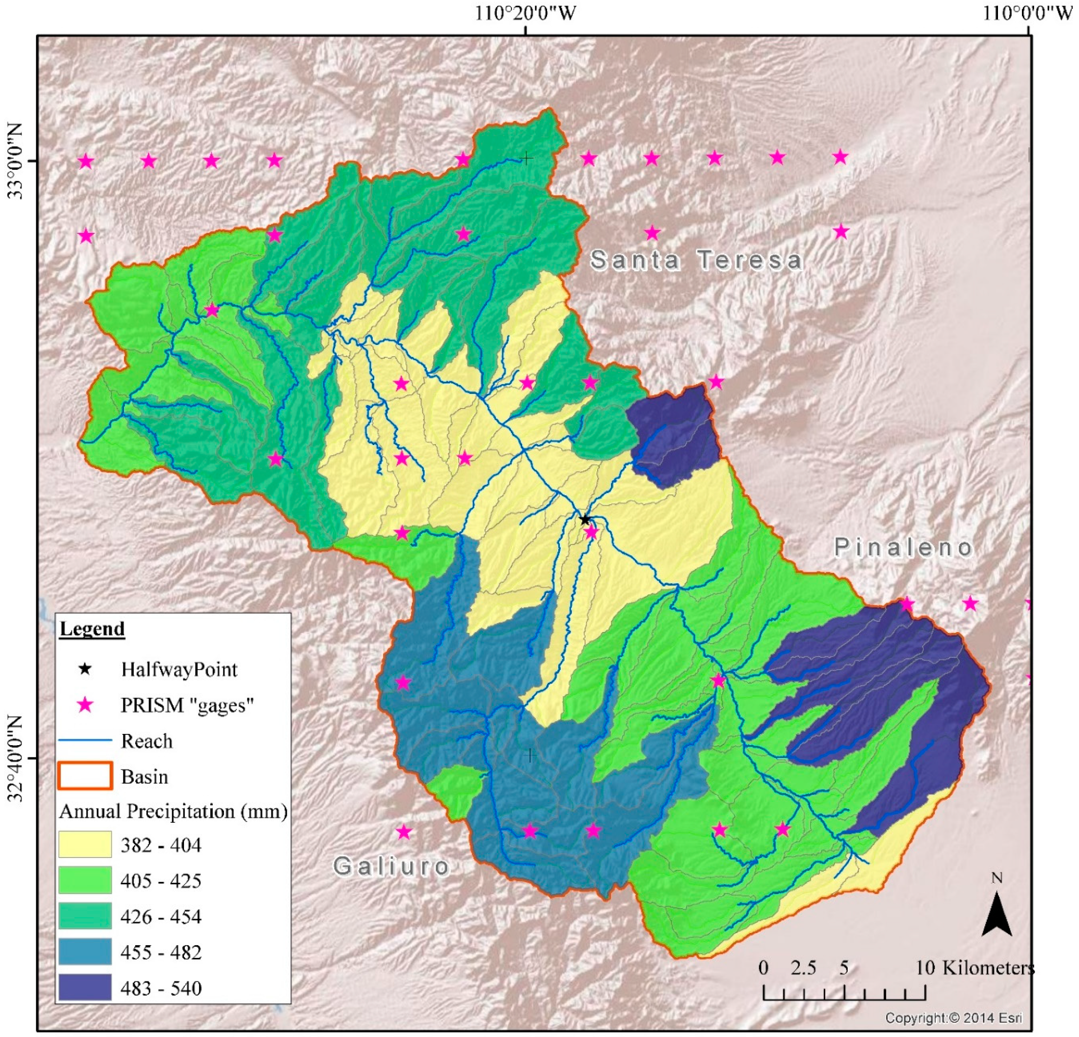
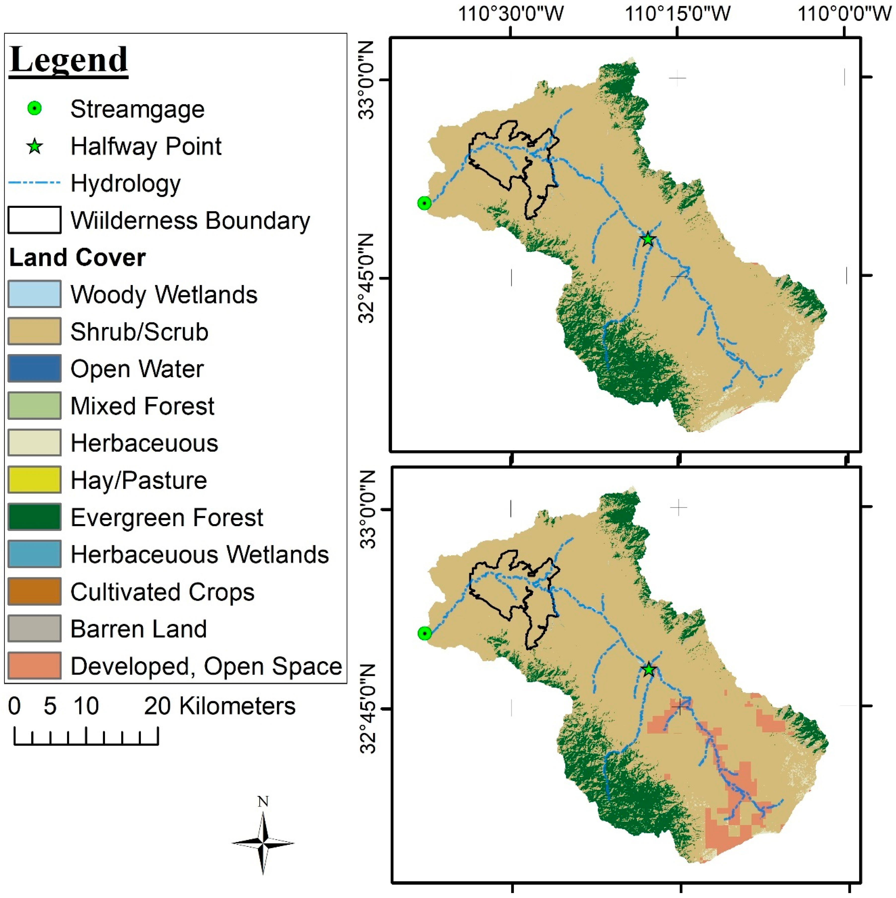
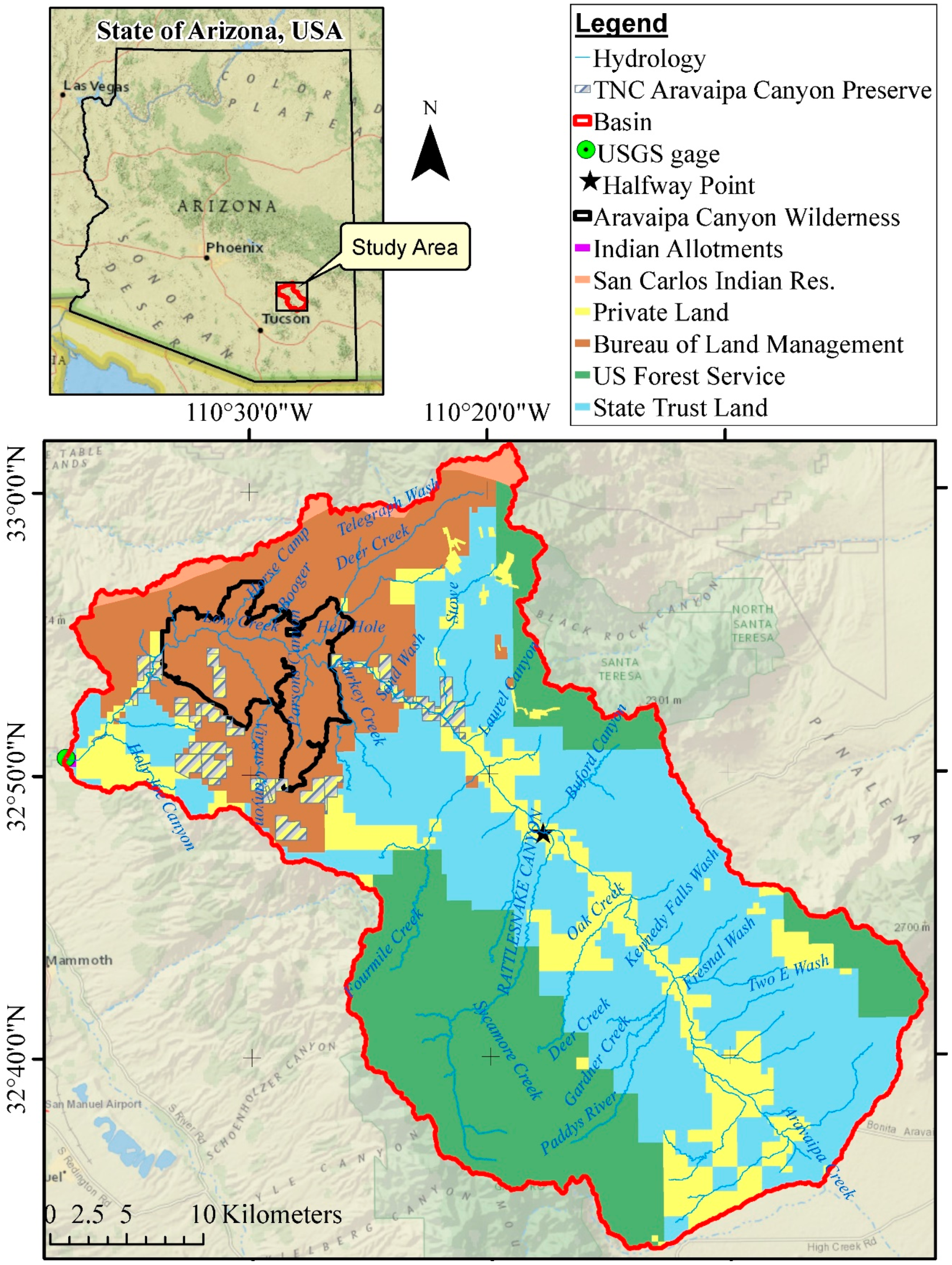
2.1. Study Area
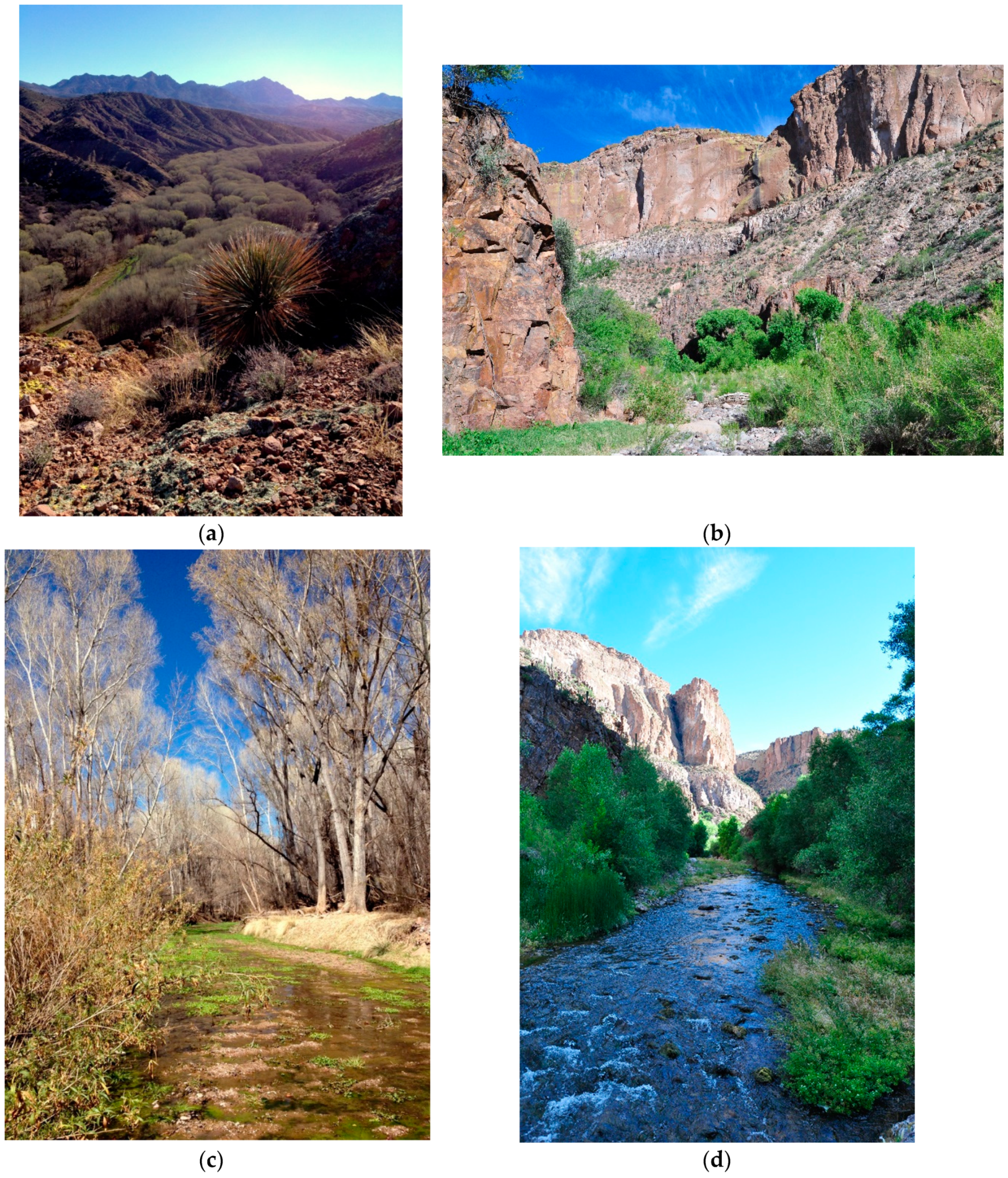
2.1.1. Environmental Setting
2.1.2. Ecosystem Services
2.2. Hydrological Model Application
SWAT Model Development and Parametrization
2.3. Scenario Assessment
3. Results
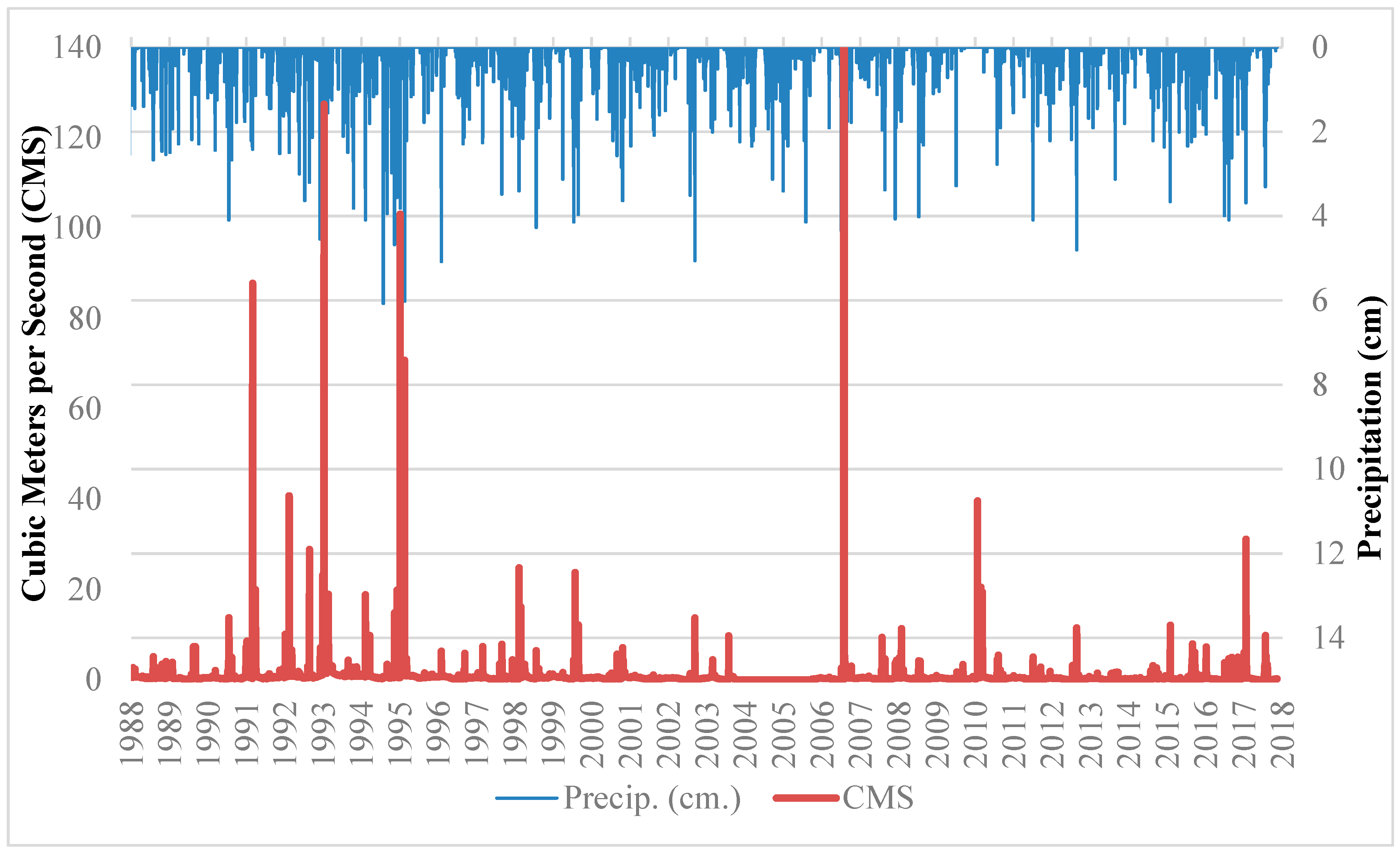
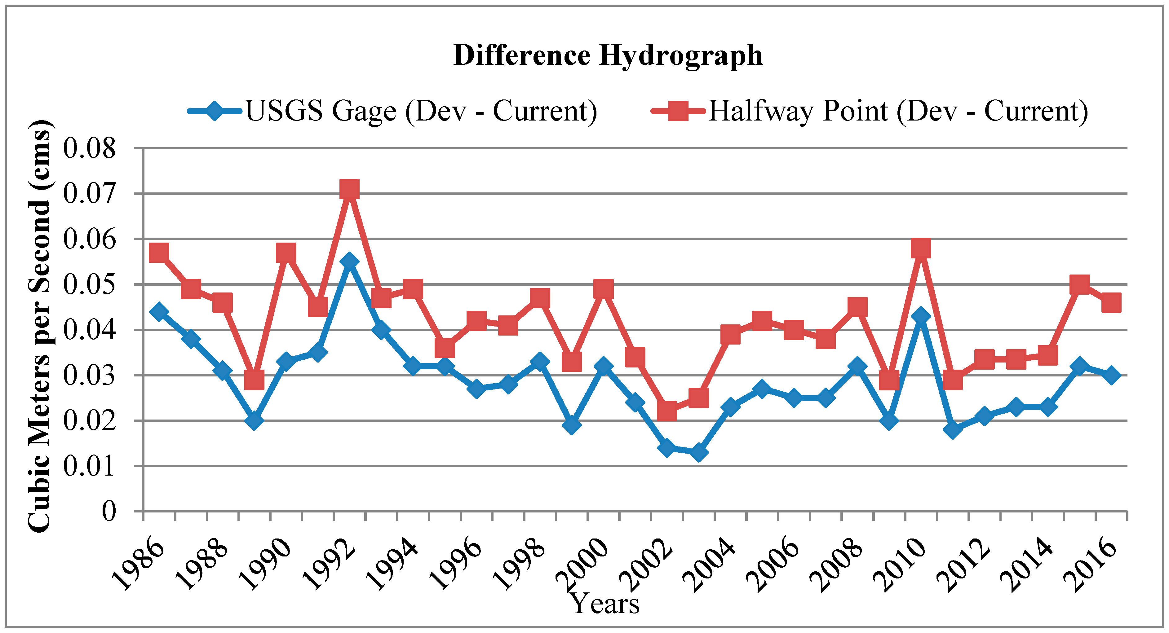
3.1. Discharge
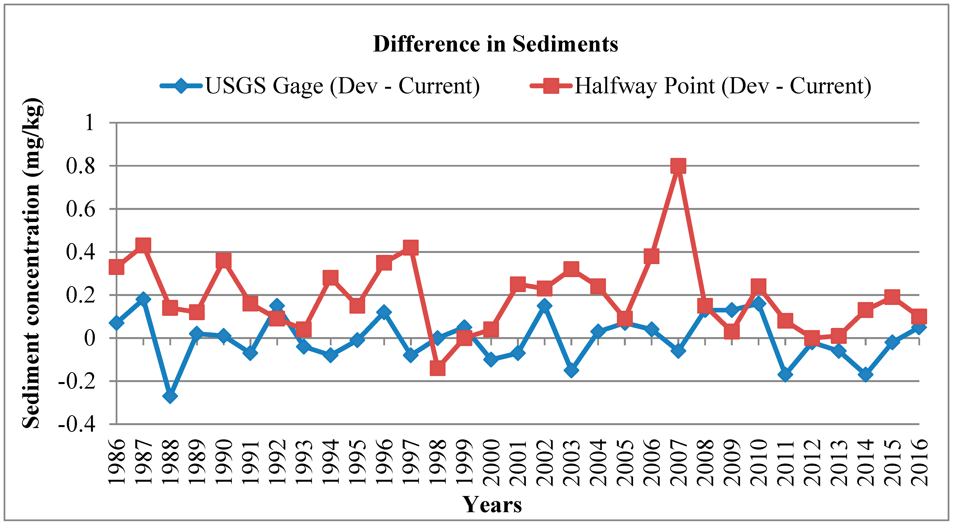
3.2. Sedimentation
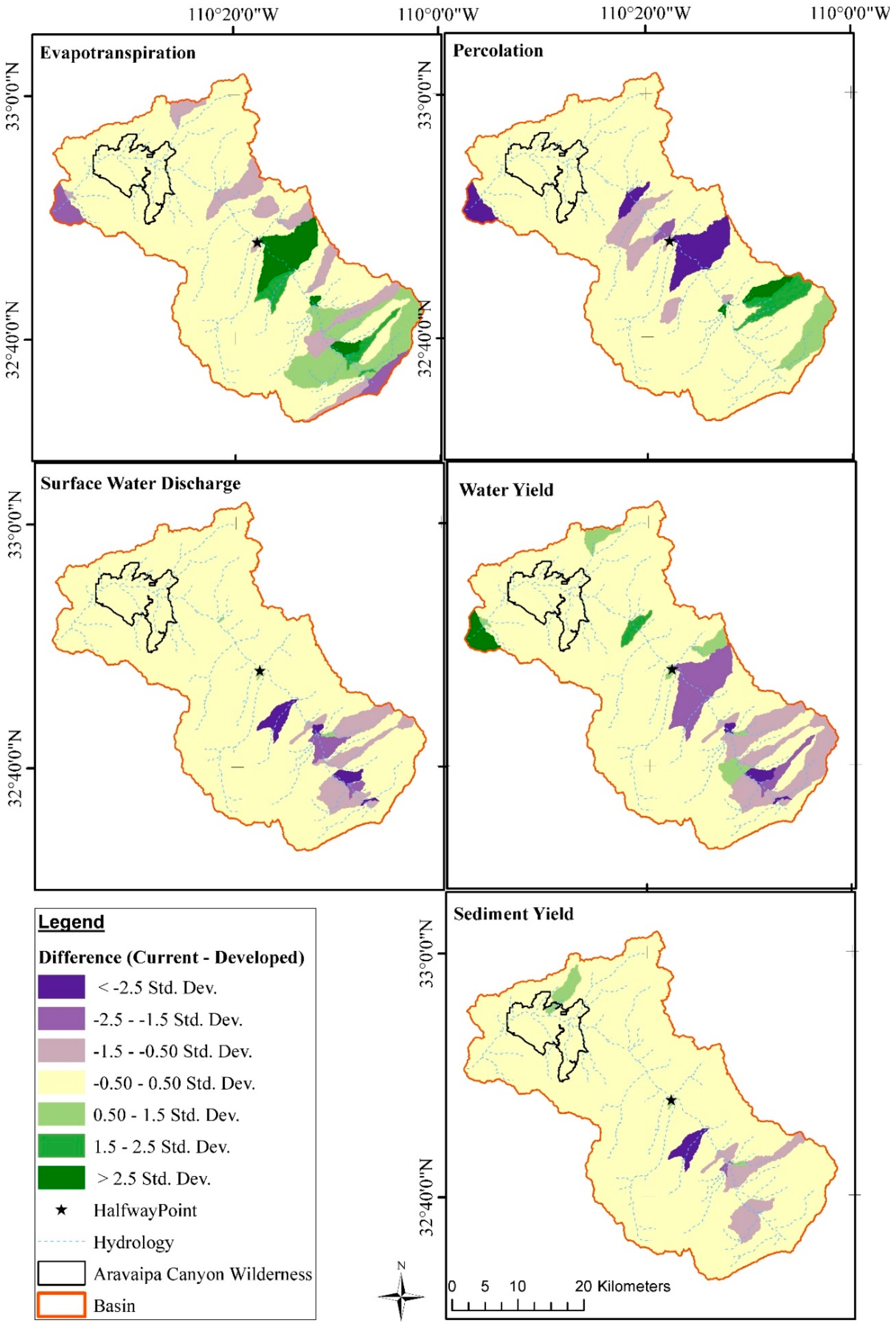
3.3. Spatial Distribution
3.4. Basin-wide Change
4. Discussion
5. Conclusions
Author Contributions
Funding
Acknowledgments
Conflicts of Interest
References
- Brown, D.G.; Johnson, K.M.; Loveland, T.R.; Theobald, D.M. Rural land-use trends in the conterminous United States, 1950–2000. Ecol. Appl. 2005, 15, 1851–1863. [Google Scholar] [CrossRef]
- Sheridan, T.E. Cows, Condos, and the Contested Commons: The Political Ecology of Ranching on the Arizona-Sonora Borderlands. Hum. Organ. 2001, 60, 141–152. [Google Scholar] [CrossRef]
- Villarreal, M.L.; Norman, L.M.; Boykin, K.G.; Wallace, C.S.A. Biodiversity losses and conservation trade-offs: Assessing future urban growth scenarios for a North American trade corridor. Int. J. Biodivers. Sci. Ecosyst. Serv. Manag. 2013, 9, 90–103. [Google Scholar] [CrossRef]
- Mitchell, J.E.; Knight, R.L.; Camp, R.J. Landscape attributes of subdivided ranches. Rangelands 2002, 24, 3–9. [Google Scholar] [CrossRef]
- Hansen, A.J.; Knight, R.L.; Marzluff, J.M.; Powell, S.; Brown, K.; Gude, P.H.; Jones, K. Effects of Exurban Development on Biodiversity: Patterns, Mechanisms, and Research Needs. Ecol. Appl. 2005, 15, 1893–1905. [Google Scholar] [CrossRef]
- Maestas, J.D.; Knight, R.L.; Gilgert, W.C. Biodiversity across a rural land-use gradient. Conserv. Biol. 2003, 17, 1425–1434. [Google Scholar] [CrossRef]
- Theobald, D.M.; Miller, J.R.; Hobbs, N.T. Estimating the cumulative effects of development on wildlife habitat. Landsc. Urban Plan. 1997, 39, 25–36. [Google Scholar] [CrossRef]
- Leopold, L.B. Hydrology for Urban Land Planning: A Guidebook on the Hydrologic Effects of Urban Land Use; Circular; U.S. Geological Survey: Washington, DC, USA, 1968.
- Ellingson, C.T. The Hydrology of Aravaipa Creek, Southeastern Arizona; M.S. Hydrology and Water Resources, The University of Arizona: Tucson, AZ, USA, 1980. [Google Scholar]
- Havstad, K.M.; Peters, D.P.C.; Skaggs, R.; Brown, J.; Bestelmeyer, B.; Fredrickson, E.; Herrick, J.; Wright, J. Ecological services to and from rangelands of the United States. Ecol. Econ. 2007, 64, 261–268. [Google Scholar] [CrossRef]
- Charnley, S.; Sheridan, T.E.; Nabhan, G.P. Stitching the West Back Together: Conservation of Working Landscapes; Summits: Environmental Science, Law, and Policy; The University of Chicago Press: Chicago, IL, USA; London, UK, 2014; ISBN 978-0-226-16568-4. [Google Scholar]
- Norman, L.M.; Guertin, D.; Feller, M. A Coupled Model Approach to Reduce Nonpoint-Source Pollution Resulting from Predicted Urban Growth: A Case Study in the Ambos Nogales Watershed. Urban Geogr. 2008, 29, 496–516. [Google Scholar] [CrossRef]
- Norman, L.M.; Tallent-Halsell, N.; Labiosa, W.; Weber, M.; McCoy, A.; Hirschboeck, K.; Callegary, J.; van Riper, C.; Gray, F. Developing an Ecosystem Services Online Decision Support Tool to Assess the Impacts of Climate Change and Urban Growth in the Santa Cruz Watershed; Where We Live, Work, and Play. Sustainability 2010, 2, 2044–2069. [Google Scholar] [CrossRef] [Green Version]
- Norman, L.M.; Villarreal, M.; Niraula, R.; Meixner, T.; Frisvold, G.; Labiosa, W. Framing Scenarios of Binational Water Policy with a Tool to Visualize, Quantify and Valuate Changes in Ecosystem Services. Water 2013, 5, 852–874. [Google Scholar] [CrossRef] [Green Version]
- Norman, L.M.; Guertin, D.P.; Feller, M. An approach to prevent nonpoint-source pollutants and support sustainable development in the Ambos Nogales transboundary watershed. In Proceedings of a USGS Workshop on Facing Tomorrow’s Challenges Along the US-Mexico Border—Monitoring, Modeling, and Forecasting Change Within the Arizona; US Geological Survey Circular: Tucson, AZ, USA, 2008. [Google Scholar]
- Norman, L.M.; Villarreal, M.L.; Lara-Valencia, F.; Yuan, Y.; Nie, W.; Wilson, S.; Amaya, G.; Sleeter, R. Mapping socio-environmentally vulnerable populations access and exposure to ecosystem services at the U.S.–Mexico borderlands. Appl. Geogr. 2012, 34, 413–424. [Google Scholar] [CrossRef]
- Perkl, R.; Norman, L.M.; Mitchell, D.; Feller, M.; Smith, G.; Wilson, N.R. Urban Growth and Connectivity Threats Assessment at Saguaro National Park, Arizona, USA. J. Land Use Sci. 2018, 13, 102–117. [Google Scholar] [CrossRef]
- Belsky, A.J.; Matzke, A.; Uselman, S. Survey of livestock influences on stream and riparian ecosystems in the western United States. J. Soil Water Conserv. 1999, 54, 419–431. [Google Scholar]
- Fleischner, T.L. Ecological Costs of Livestock Grazing in Western North America. Conserv. Biol. 1994, 8, 629–644. [Google Scholar] [CrossRef]
- Brown, J.H.; McDonald, W. Livestock grazing and conservation on southwestern rangelands. Conserv. Biol. 1995, 9, 1644–1647. [Google Scholar] [CrossRef]
- Herrero, M.; Thornton, P.K.; Gerber, P.; Reid, R.S. Livestock, livelihoods and the environment: Understanding the trade-offs. Curr. Opin. Environ. Sustain. 2009, 1, 111–120. [Google Scholar] [CrossRef]
- Duniway, M.C.; Geiger, E.L.; Minnick, T.J.; Phillips, S.L.; Belnap, J. Insights from Long-Term Ungrazed and Grazed Watersheds in a Salt Desert Colorado Plateau Ecosystem. Rangel. Ecol. Manag. 2018, 71, 492–505. [Google Scholar] [CrossRef]
- Dale, V.; Archer, S.; Chang, M.; Ojima, D. Ecological Impacts and Mitigation Strategies for Rural Land Management. Ecol. Appl. 2005, 15, 1879–1892. [Google Scholar] [CrossRef]
- Bestelmeyer, B.T.; Briske, D.D. Grand Challenges for Resilience-Based Management of Rangelands. Rangel. Ecol. Manag. 2012, 65, 654–663. [Google Scholar] [CrossRef] [Green Version]
- Brauman, K.A. Hydrologic ecosystem services: Linking ecohydrologic processes to human well-being in water research and watershed management: Hydrologic ecosystem services. Wiley Interdiscip. Rev. Water 2015, 2, 345–358. [Google Scholar] [CrossRef]
- Maczko, K.; Tanaka, J.A.; Breckenridge, R.; Hidinger, L.; Heintz, H.T.; Fox, W.E.; Kreuter, U.P.; Duke, C.S.; Mitchell, J.E.; McCollum, D.W. Rangeland Ecosystem Goods and Services: Values and Evaluation of Opportunities for Ranchers and Land Managers. Rangelands 2011, 33, 30–36. [Google Scholar] [CrossRef] [Green Version]
- Wilcox, B.P.; Le Maitre, D.; Jobbagy, E.; Wang, L.; Breshears, D.D. Ecohydrology: Processes and Implications for Rangelands. In Rangeland Systems; Springer: Berlin/Heidelberg, Germany, 2017; pp. 85–129. [Google Scholar]
- Bohlen, P.J.; Lynch, S.; Shabman, L.; Clark, M.; Shukla, S.; Swain, H. Paying for environmental services from agricultural lands: An example from the northern Everglades. Front. Ecol. Environ. 2009, 7, 46–55. [Google Scholar] [CrossRef]
- Villarreal, M.L.; Norman, L.M.; Labiosa, W.B. Assessing the vulnerability of human and biological communities to changing ecosystem services using a GIS-based multi-criteria decision support tool. In Proceedings of the 2012 International Congress on Environmental Modelling and Software (iEMSs), Leipzig, Germany, 1 July 2012; Managing Resources of a Limited Planet: Pathways and Visions under Uncertainty, Sixth Biennial Meeting. Seppelt, R., Voinov, A.A., Lange, S., Bankamp, D., Eds.; pp. 427–434. [Google Scholar]
- Hadley, D.; Warshall, P.; Bufkin, D. Environmental Change in ARAVAIPA, 1870–1970: An Ethnoecological Survey; Cultural Resource Series; Arizona State Office of the Bureau of Land Management: Phoenix, AZ, USA, 1991.
- Minckley, W.L. Ecological Studies of Aravaipa Creek, Central Arizona, Relative to Past, Present and Future Land Uses; Bureau of Land Management: Safford, AZ, USA, 1981.
- USBLM. Aravaipa Ecosystem Management Plan and Environmental Assessment; Prepared by U.S. Department of the Interior, Bureau of Land Management, Safford Field Office, Arizona; Arizona Game and Fish Department; Region V. The Nature Conservancy; Arizona Chapter; Bureau of Land Management, Safford Field Office: Arizona, AZ, USA, 2015.
- Adar, E.M.; Neuman, S.P. Estimation of spatial recharge distribution using environmental isotopes and hydrochemical data, II. Application to Aravaipa Valley in Southern Arizona, U.S.A. J. Hydrol. 1988, 97, 279–302. [Google Scholar] [CrossRef]
- Moore, S.D.; Wilkosz, M.E.; Brickler, S.K. The recreational impact of reducing the” Laughing Waters” of Aravaipa Creek, Arizona. Rivers 1990, 1, 43–50. [Google Scholar]
- Norman, L.M.; Haberstich, M.; Niraula, R.; Wilson, N.R.; Middleton, B.R. Development Implication on Hydrologic Ecosystem Services in the Aravaipa Canyon Watershed, SE Arizona; US Geological Survey: Tucson, AZ, USA, 2018; p. 51.
- Arizona Department of Water Resources Hydrology of the Aravaipa Canyon Basin. Available online: http://www.azwater.gov/AzDWR/StatewidePlanning/WaterAtlas/SEArizona/Hydrology/AravaipaCanyon.htm (accessed on 28 March 2018).
- Holmes, M.A. Maps Showing Groundwater Conditions in Aravaipa Canyon Basin, Pinal and Graham Counties, Arizona, 1996. Arizona Department of Water Resources: Phoenix, AZ, USA, 2003. Available online: https://new.azwater.gov/content/hms-no-33 (accessed on 15 April 2019).
- Freethey, G.W.; Anderson, T.W. Predevelopment Hydrologic Conditions in the Alluvial Basins of Arizona and Adjacent Parts of California and New Mexico; Hydrologic Atlas; US Geological Survey: Reston, VA, USA, 1986.
- Weber, M.A.; Berrens, R.P. Value of Instream Recreation in the Sonoran Desert. J. Water Resour. Plan. Manag. 2006, 132, 53–60. [Google Scholar] [CrossRef]
- Hirschberg, D.M.; Pitts, G.S. Digital Geologic Map of Arizona: A Digital Database Derived from the 1983 Printing of the Wilson, Moore, and Cooper 1:500,000-Scale Map; Open-File Report 00-409; US Geological Survey: Reston, VA, USA, 2000; p. 67.
- Arizona Department of Water Resources Section 3.14 Willcox Basin. In Arizona Water Atlas; Arizona Department of Water Resources: Phoenix, AZ, USA, 2009; Volume 3, pp. 534–602.
- Millennium Ecosystem Assessment. Ecosystems and Human Well-Being; Island Press: Washington, DC, USA, 2005; Volume 5. [Google Scholar]
- Abbey, E. In the Land of “Laughing Waters”. The New York Times, 3 January 1982. [Google Scholar]
- Logsdon, R.A.; Chaubey, I. A quantitative approach to evaluating ecosystem services. Ecol. Model. 2013, 257, 57–65. [Google Scholar] [CrossRef]
- Villarreal, M.L.; Petrakis, R.E. Conflation and aggregation of spatial data improve predictive models for species with limited habitats: A case of the threatened yellow-billed cuckoo in Arizona, USA. Appl. Geogr. 2014, 47, 57–69. [Google Scholar] [CrossRef]
- Eby, L.A.; Fagan, W.F.; Minckley, W.L. Variability and Dynamics of a Desert Stream Community. Ecol. Appl. 2003, 13, 1566–1579. [Google Scholar] [CrossRef]
- Deacon, J.E.; Minckley, W.L. Desert fishes. In Desert Biology; Brown, G.W., Jr., Ed.; Academic Press: New York, NY, USA, 1974; Volume 2, pp. 385–488. [Google Scholar]
- Arnold, J.G.; Srinivasan, R.; Muttiah, R.S.; Williams, J.R. Large Area Hydrologic Modeling and Assessment Part I: Model Development1. JAWRA J. Am. Water Resour. Assoc. 1998, 34, 73–89. [Google Scholar] [CrossRef]
- Neitsch, S.L.; Arnold, J.G.; Kiniry, J.R.; Williams, J.R. Soil Water Assessment Tool: Theoretical Documentation; Version 2009; Texas Water Resources Institute: College Station, TX, USA, 2009. [Google Scholar]
- Almendinger, J.E.; Murphy, M.S.; Ulrich, J.S. Use of the Soil and Water Assessment Tool to Scale Sediment Delivery from Field to Watershed in an Agricultural Landscape with Topographic Depressions. J. Environ. Qual. 2014, 43, 9–17. [Google Scholar] [CrossRef] [PubMed]
- Miller, S.N.; Semmens, D.J.; Goodrich, D.C.; Hernandez, M.; Miller, R.C.; Kepner, W.G.; Guertin, D.P. The Automated Geospatial Watershed Assessment tool. Environ. Model. Softw. 2007, 22, 365–377. [Google Scholar] [CrossRef]
- Niraula, R.; Kalin, L.; Wang, R.; Srivastava, P. Determining Nutrient and Sediment Critical Source Areas with SWAT: Effect Of Lumped Calibration. Trans. ASABE 2011, 55, 137–147. [Google Scholar] [CrossRef]
- Niraula, R.; Norman, L.M.; Meixner, T.; Callegary, J. Multi-gauge Calibration for modeling the Semi-Arid Santa Cruz Watershed in Arizona-Mexico Border Area Using SWAT. Air Soil Water Res. 2012, 5. [Google Scholar] [CrossRef]
- Yuan, Y.; Nie, W. Problems and Prospects of SWAT Model Application on an Arid/Semiarid Watershed in Arizona. In Proceedings of the Sustainable Water Resources in a Changing Environment, Reno, NV, USA, 19–23 April 2015. [Google Scholar]
- Goodrich, D.C.; Burns, I.S.; Unkrich, C.L.; Semmens, D.J.; Guertin, D.P.; Hernandez, M.; Yatheendradas, S.; Kennedy, J.; Levick, L.R. KINEROS2/AGWA: Model use, calibration, and validation. Trans. ASABE 2012, 55, 1561–1574. [Google Scholar] [CrossRef]
- Kepner, W.G.; Semmens, D.J.; Bassett, S.D.; Mouat, D.A.; Goodrich, D.C. Scenario Analysis for the San Pedro River, Analyzing Hydrological Consequences of a Future Environment. Environ. Monit. Assess. 2004, 94, 115–127. [Google Scholar] [CrossRef]
- Niraula, R.; Meixner, T.; Norman, L.M. Determining the importance of model calibration for forecasting absolute/relative changes in streamflow from LULC and climate changes. J. Hydrol. 2015, 522, 439–451. [Google Scholar] [CrossRef]
- Soil Survey Staff, Natural Resources Conservation Service, United States Department of Agriculture Soil Survey Geographic (SSURGO) Database for Arizona. Available online: https://websoilsurvey.nrcs.usda.gov/ (accessed on 1 March 2018).
- Wickham, J.; Homer, C.; Vogelmann, J.; McKerrow, A.; Mueller, R.; Herold, N.; Coulston, J. The Multi-Resolution Land Characteristics (MRLC) Consortium—20 years of development and integration of USA national land cover data. Remote Sens. 2014, 6, 7424–7441. [Google Scholar] [CrossRef]
- Daly, C.; Taylor, G.H.; Gibson, W.P. The PRISM approach to mapping precipitation and temperature. In Proceedings of the 10th Conference on Applied Climatology, American Meteorology Society, Reno, NV, USA, 19–23 October 1997; pp. 10–12. [Google Scholar]
- Arnold, J.G.; Kiniry, J.R.; Srinivasan, R.; Williams, J.R.; Haney, E.B.; Neitsch, S.L. Soil and Water Assessment Tool Input/Output Documentation Versio 2012; Texas Water Resources Institute: College Station, TX, USA, 2012. [Google Scholar]
- Norman, L.M.; Brinkerhoff, F.; Gwilliam, E.; Guertin, D.P.; Callegary, J.; Goodrich, D.C.; Nagler, P.L.; Gray, F. Hydrologic Response of Streams Restored with Check Dams in the Chiricahua Mountains, Arizona. River Res. Appl. 2015, 32, 519–527. [Google Scholar] [CrossRef] [Green Version]
- Norman, L.M.; Callegary, J.B.; Lacher, L.J.; Wilson, N.R.; Fandel, C.A.; Forbes, B.; Swetnam, T. Impacts of Restoration on Groundwater Recharge at the Babocomari Ranch, SE Arizona, USA. Water 2019, 11, 381. [Google Scholar] [CrossRef]
- Schreiner-McGraw, A.P.; Vivoni, E.R. On the Sensitivity of Hillslope Runoff and Channel Transmission Losses in Arid Piedmont Slopes. Water Resour. Res. 2018, 54, 4498–4518. [Google Scholar] [CrossRef]
- Nie, W.; Yuan, Y.; Kepner, W.; Nash, M.S.; Jackson, M.; Erickson, C. Assessing impacts of Landuse and Landcover changes on hydrology for the upper San Pedro watershed. J. Hydrol. 2011, 407, 105–114. [Google Scholar] [CrossRef]
- Norman, L.M.; Niraula, R. Model analysis of check dam impacts on long-term sediment and water budgets in Southeast Arizona, USA. Ecohydrol. Hydrobiol. 2016, 16, 125–137. [Google Scholar] [CrossRef]
- Norman, L.M. Modeling Land Use Change and Associate Water Quality Impacts in the Ambos Nogales Watershed, United States-Mexico Border. Ph.D. Thesis, The University of Arizona, Tucson, AZ, USA, 2005. [Google Scholar]
- Norman, L.M. United States-Mexican Border Watershed Assessment: Modeling Nonpoint Source Pollution in Ambos Nogales. J. Borderl. Stud. 2007, 22, 79–97. [Google Scholar] [CrossRef]
- Norman, L.M.; Huth, H.; Levick, L.; Shea Burns, I.; Phillip Guertin, D.; Lara-Valencia, F.; Semmens, D. Flood hazard awareness and hydrologic modelling at Ambos Nogales, United States–Mexico border. J. Flood Risk Manag. 2010, 3, 151–165. [Google Scholar] [CrossRef]
- Norman, L.M.; Levick, L.R.; Guertin, D.P.; Callegary, J.B.; Quintanar Guadarrama, J.; Zulema Gil Anaya, C.; Prichard, A.; Gray, F.; Castellanos, E.; Tepezano, E.; et al. Nogales Flood Detention Study; Open-File Report 2010-1262; US Geological Survey: Reston, VA, USA, 2010; p. 112.
- Norman, L.M.; Villarreal, M.L.; Pulliam, H.R.; Minckley, R.; Gass, L.; Tolle, C.; Coe, M. Remote sensing analysis of riparian vegetation response to desert marsh restoration in the Mexican Highlands. Ecol. Eng. 2014, 70, 241–254. [Google Scholar] [CrossRef] [Green Version]
- Newman, B.D.; Wilcox, B.P.; Archer, S.R.; Breshears, D.D.; Dahm, C.N.; Duffy, C.J.; McDowell, N.G.; Phillips, F.M.; Scanlon, B.R.; Vivoni, E.R. Ecohydrology of water-limited environments: A scientific vision: OPINION. Water Resour. Res. 2006, 42. [Google Scholar] [CrossRef]
- Winter, T.C.; Harvey, J.W.; Franke, O.L.; Alley, W.M. Ground Water and Surface Water: A Single Resource; U.S. Geological Survey Circular: Denver, CO, USA, 1998; ISBN 0-607-89339-7.


| Current | Developed | Difference | Units | % Change | |
|---|---|---|---|---|---|
| PRECIP | 425.4 | 425.4 | 0 | MM | 0 |
| SURFACE RUNOFF DISCHARGE (Q) | 18.13 | 18.99 | 0.86 | MM | 5 |
| LATERAL SOIL Q | 83.02 | 82.71 | −0.31 | MM | 0 |
| TOTAL WATER YIELD | 104.09 | 104.71 | 0.62 | MM | 1 |
| GROUNDWATER (SHALLOW AQUIFER) Q | 2.3 | 2.35 | 0.05 | MM | 2 |
| DEEP AQUIFER RECHARGE | 0.63 | 0.64 | 0.01 | MM | 2 |
| PERCOLATION OUT OF SOIL | 12.68 | 12.84 | 0.16 | MM | 1 |
| TOTAL AQUIFER RECHARGE | 12.7 | 12.86 | 0.16 | MM | 1 |
| EVAPOTRANSPIRATION | 311.3 | 310.6 | −0.7 | MM | 0 |
| TOTAL SEDIMENT LOADING | 2.47 | 2.52 | 0.05 | T/HA | 2 |
| Category | Ecosystem Service | SWAT Output | Local Response |
|---|---|---|---|
| Provisioning | Water | SURFACE RUNOFF Q | Increase |
| Water | TOTAL AQ RECHARGE | Increase | |
| Food (crops/rangeland) | ET | Decrease | |
| Food (crops/rangeland) | NUTRIENTS in Soil | Decrease | |
| Fuel | ET | Decrease | |
| Soil-Moisture | LATERAL SOIL Q | Decrease | |
| Regulating | Water quality | TOTAL SEDIMENT LOADING | Decrease |
| Erosion control | TOTAL SEDIMENT LOADING | Decrease | |
| Flood control | SURFACE RUNOFF Q | Decrease | |
| Supporting | Habitat (in-stream) | Dependent on Water Provisioning and Water Quality Regulating | Change |
| Habitat (on land) | Dependent on Food (crops/rangeland) Provisioning | Change | |
| Habitat (on land) | Dependent on Erosion Control Regulating | Change | |
| Cultural | Recreation (hiking, hunting, birding) | Dependent on Water Provisioning | Change |
| Intrinsic (biodiversity, societal value) | Dependent on Water Provisioning | Change | |
| Historical | Dependent on Water Provisioning | Change |
© 2019 by the authors. Licensee MDPI, Basel, Switzerland. This article is an open access article distributed under the terms and conditions of the Creative Commons Attribution (CC BY) license (http://creativecommons.org/licenses/by/4.0/).
Share and Cite
Norman, L.M.; Villarreal, M.L.; Niraula, R.; Haberstich, M.; Wilson, N.R. Modelling Development of Riparian Ranchlands Using Ecosystem Services at the Aravaipa Watershed, SE Arizona. Land 2019, 8, 64. https://doi.org/10.3390/land8040064
Norman LM, Villarreal ML, Niraula R, Haberstich M, Wilson NR. Modelling Development of Riparian Ranchlands Using Ecosystem Services at the Aravaipa Watershed, SE Arizona. Land. 2019; 8(4):64. https://doi.org/10.3390/land8040064
Chicago/Turabian StyleNorman, Laura M., Miguel L. Villarreal, Rewati Niraula, Mark Haberstich, and Natalie R. Wilson. 2019. "Modelling Development of Riparian Ranchlands Using Ecosystem Services at the Aravaipa Watershed, SE Arizona" Land 8, no. 4: 64. https://doi.org/10.3390/land8040064
APA StyleNorman, L. M., Villarreal, M. L., Niraula, R., Haberstich, M., & Wilson, N. R. (2019). Modelling Development of Riparian Ranchlands Using Ecosystem Services at the Aravaipa Watershed, SE Arizona. Land, 8(4), 64. https://doi.org/10.3390/land8040064