Abstract
The growing demand for biofuel production increased agricultural activities in South Dakota, leading to the conversion of grassland to cropland. Although a few land change studies have been conducted in this area, they lacked spatial details and were based on the traditional bi-temporal change detection that may return incorrect rates of conversion. This study aimed to provide a more complete view of land conversion in South Dakota using a trajectory-based analysis that considers the entire satellite-based land cover/land use time series to improve change detection. We estimated cropland expansion of 5447 km2 (equivalent to 14% of the existing cropland area) between 2007 and 2015, which matches much more closely the reports from the National Agriculture Statistics Service—NASS (5921 km2)—and the National Resources Inventory—NRI (5034 km2)—than an estimation from the bi-temporal approach (8018 km2). Cropland gains were mostly concentrated in 10 counties in northern and central South Dakota. Urbanizing Lincoln County, part of the Sioux Falls metropolitan area, is the only county with a net loss in cropland area over the study period. An evaluation of land suitability for crops using the Soil Survey Geographic Database (SSURGO) indicated a scarcity in high-quality arable land available for cropland expansion.
1. Introduction
Agriculture is the leading industry of South Dakota, contributing approximate $22 billion to the state’s economy each year [1]. Both crop production and livestock play important roles, sharing 60.7% and 39.3% of the total agricultural revenue. Over the past decade, the growing demand for biofuel production led to a considerable expansion of cropland area in South Dakota (increase of 1–5% annually [2]), especially for corn/maize (for corn-based ethanol) and soybean (for biodiesel) [2,3]. Corn/maize and soybean are South Dakota’s two largest crops by area, accounting for 68% of the harvested field crops in 2017 (43,370 km2) [4]. Conversion from grassland or wetland to cropland can alter the landscape [2,3] and hurt the ecosystem as well as the environment [5,6,7,8,9,10].
Several efforts have been made to characterize land dynamics in the U.S. Northern Great Plains (spans over multiple states, including the entire South Dakota). Most extant studies take a bi-temporal “snapshot” approach [2,3,11,12] that only compares data between two points in time and disregards data from intermediate years. The bi-temporal approach does not capture the regular rotation of lands into and out of cultivation and, thus, may retrieve an incorrect rate of conversion [13]. There are only two studies that provide more temporal context to land change analysis in South Dakota [13,14]. However, one examined land change only for a brief period (2008–2012) [13], while the other provided a long-term analysis (1984–2016) but covered only a portion of the state (Landsat path 30, rows 28–29) [14]. Although the extant research has reported different amounts of land change, each study showed considerable losses of grassland with conversion to cropland (mostly corn/maize and soybean) in the Northern Great Plains, especially east of the Missouri river.
Only one study has evaluated land change exclusively in South Dakota [3]. However, that study did not provide adequate spatial details about the changes. Since accurate geospatial accounts of land use change are critical in assessing long-term risk of the conversions, this paper aims to provide a more complete view of land conversion in South Dakota by characterizing the dominant land cover transition from 2006 to 2016 and its spatiotemporal patterns. To overcome the limitations of the bi-temporal change detection, we propose a trajectory-based approach that considers the entire land cover/land use time series to determine if there was actual land change at a particular location. First, land cover/land use (LCLU) maps were generated annually from 2006 to 2016 at 30-meter resolution (eleven maps in total) using the phenometric-based classification described in [15]. This LCLU dataset allowed us to analyze land changes in the study area over the past decade. The results were then compared against various official data sources released by the United States Department of Agriculture (USDA).
2. Methods
2.1. Generation of Land Cover/Land Use Dataset
To characterize land changes in the study area, a fine spatiotemporal resolution land cover dataset with just three broad categories (“cropland”, “grassland”, and “others”) was generated using the phenometric-based classification as described in [15]. First, at each pixel, the seasonal variation of EVI (Enhanced Vegetation Index) time series derived from Landsat Collection-1 Surface Reflectance product (courtesy of the U.S. Geological Survey) was modeled as a downward-arching convex quadratic function [16,17] of accumulated growing degree-days (AGDD) derived from MODIS (MODerate resolution Imaging Spectrometer) level-3 V005 global Land Surface Temperature and Emissivity eight-day composite products [18,19]. Then, from the fitted model parameter coefficients, a suite of 16 metrics (Table S1) was derived to serve as input for the land cover/land use classification task using a Random Forest Classifier (RFC).
The USDA National Agriculture Statistics Service (NASS) Cropland Data Layer (CDL) [20] was used to select training and testing pixels (the sample dataset) for the RFC models—despite known issues with the CDL [21,22]—due to a scarcity of ground observations. To increase the accuracy of sample dataset, only pixels that were surrounded by eight pixels of the same cover type and repeated cover type at least once in the study period were selected. Because the generated land cover maps contain just three broad categories, the CDL layers were regrouped into those classes to be used in the sample selection.
LCLU classifications were performed annually on county basis to improve accuracy [23]. From each county-year sample pool, multiple stratified random sample datasets were selected, each covering 0.25% of the county area [15]. For each county-year, twenty RFC models were performed and ensembled to retrieve a final LCLU map. The accuracies of the generated land cover/ land use maps were examined using a rich reference dataset that contains 14,400 points in each of just three years: 2006, 2012, 2014 [21]. In addition, predicted land cover areas from this study were compared with those from existing studies and databases.
Due to cloud/snow contamination or band gaps caused by failure of the Scan Line Corrector on Landsat 7 ETM+ [24], there were not enough observations (EVI data points) over a year to fit the convex quadratic function at certain pixels at image edges. The phenometric-based classification was not able to assign cover types for those pixels, thereby generating gaps in the cover maps [15]. In order to create seamless maps for change detection, the gaps of a current year were filled by land cover information from the two adjacent years, favoring the previous year’s information. For example, missing land cover information from 2008 was first filled using the 2007 data. If there was also a data gap in 2007, the 2009 land cover information was used to fill gaps in the 2008 cover map.
2.2. Characterizing Cropland Expansion Using The Trajectory-Based Change Detection
Phenometric-based classification can generate very accurate cropland maps but may not work as well for other land covers [15]. Therefore, this analysis focused only on changes in cropland. We developed the trajectory-based approach that considered land cover information from the entire time series to determine whether land cover at a pixel shifted cover types. Since the analysis focused on characterizing cropland expansion, all land cover maps were regrouped into “cropland” and “non-cropland” (“grassland” and “others”) for the change detection.
The trajectory-based change analysis of each crop pixel is presented in Figure 1. First, land cover maps from 2006 to 2016 were stacked to create a time series. Then, the map series was converted into a binary time series with “0” for “non-cropland” and “1” for “cropland”. A binary array at each pixel indicates land cover and changes over time. To counter misclassifications in the land cover dataset, we assumed that a single year of different land cover in the entire 11-year time series was “noise”.
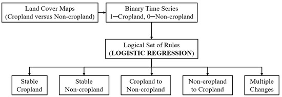
Figure 1.
The trajectory-based change detection workflow for cropland.
First, from the binary time series, locations were identified with very strong temporal signal of being “cropland” or “non-cropland”. Over 11 years, if a number of times (counts) that a pixel appeared as “cropland” was less than two, the pixel was assigned as “stable non-cropland”. Similarly, a pixel with counts of greater than nine was considered as a “stable cropland” pixel.
After masking out pixels with less than two or more than nine appearances as “cropland”, all other possible “cropland” pixels (2 ≤ “counts” ≤ 9) were subjected to further change analysis. To incorporate land formation from all eleven years of data in change detection, the logistic regression was performed on each binary time series using calendar year as the only predictor variable:
where p is the probability of the pixel appearing as “cropland” over time and (1−p) is the probability of the same pixel appearing as “non-cropland” over the same interval. From the fitted parameters (intercept and slope), we computed the p values for all years and used those values to help detect changes. If the p value of the first year (2006) was less than 0.2 and p values of the last two years (2015 and 2016) were greater than 0.8 and 0.9, respectively, a pixel was subjected as “changed” from “non-cropland” to “cropland”. On the complementary side, if p values of 2006 and 2007 were greater than 0.8 and 0.9, respectively, and the p value of 2016 was less than 0.2, a pixel was subjected as “changed” from “cropland” to “non-cropland”. All other pixels that did not meet these two conditions were further evaluated using the average probability of crop events over 11 years (pmean). If pmean was less than 0.2, a pixel was considered as a “stable non-cropland” pixel. Pixels with pmean of above 0.8 were assigned as “stable cropland”. Pixels with pmean ranging between 0.2 and 0.8 were tagged as “multiple changes”. The dominant land cover type and trend of “multiple changes” pixels are described by pmean (greater than 0.5: “cropland”, less than 0.5: “non-cropland”) and slope (greater than 0: toward “cropland”, less than “0”: toward “non-cropland”). Only changes detected from the analysis of probability were considered as “true” land cover changes. The 3×3 majority filter was applied to remove spatial noise—primarily singletons and doublets—in the land change layer.
Recall that we assumed a single mismatch in the entire land cover time series (11 years) as “noise” due to misclassification rather than an actual change. Therefore, the proposed approach did not detect changes that just happened in either 2006 or 2016. Instead, these results account for changes only between 2007 and 2015.
The suitability for crop production on stable and converted croplands was determined using Soil Survey Geographic Database (SSURGO) data [25]. Crop pixels were overlaid on the SSURGO Non-Irrigated Capability Class-Dominant Condition layer to extract land capability classes (LCC), the broadest category, which are coded from 1 to 8 indicating progressively greater limitations and narrower choices for practical use. Classes 1 to 4 are considered as arable lands, and classes 5 to 8 are suitable mainly as pasture or rangeland. We regrouped and labeled LCC 1-2 as “prime” land for cultivation, LCC 3–4 as “fragile”, and LCC 5-8 as “unsuitable” [13].
3. Results
3.1. Accuracy Assessment of Cropland Maps of South Dakota
Phenometric-based classification using the sample dataset generated from the CDL performed very well: the RFC models consistently retrieved overall accuracies of greater than 90% across counties-years (Figure S1). Consequently, general patterns of land cover/land use from the RFC models and the reclassified CDL are similar, especially for “cropland” (Figure S2, Table S2). The similarity in cropland pattern between the CDL and RFC is also shown in Figure 2 as data points (county-year cropland areas) of the scatterplot are distributed closely around the 1:1 line. From 2006 to 2009, our dataset showed slightly larger cropland areas in South Dakota (Figure 2) compared to the CDL values. After 2009, estimated cropland areas from the two datasets showed difference of less than 1% (Figure 3). The predicted land cover maps from this study and the reclassified CDL both underestimated cropland areas reported by field-based statistics from the USDA. However, these satellite-based datasets (CDL and this study) and the field-based NASS estimates showed similar temporal patterns and strong correlation to each other (Figure 3, Table S3). However, the area in “grassland” is overestimated by RFC, while the area in “others” is underestimated (Figure 2 and Figure 3). The differences in “grassland” and “others” between the CDL and this study seem to be systematic (Figure 3), possibly due to misclassification of grass-like covers in “others” (e.g., urban lawns, playing fields). While the CDL adopted the “developed” classes from the National Land Cover Database (NLCD), many “developed” pixels were classified as “grassland” or “cropland” pixels in RFC models. Those pixel classifications are not fundamentally incorrect from a land surface phenology perspective but require supplementary contextual information to shift the pixels from “grassland” (pasture/grazing use) to “others” (recreational use).
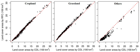
Figure 2.
County-level comparison between estimated land cover area from this study and the Cropland Data Layer (CDL). A total of 726 data points (66 counties × 11 years) were plotted.
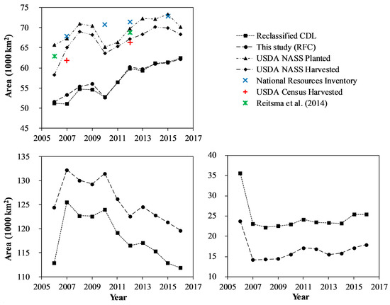
Figure 3.
State-level comparison between estimated land cover areas from this study (Random Forest Classifier; RFC) and other data sources. Both United States Department of Agriculture (USDA) National Agriculture Statistics Service (NASS) Planted/ Harvested and Census of Agriculture for South Dakota data were retrieved from the NASS website [26,27,28] with no accuracy information. The 95% confident interval (CI) for 2007, 2010, 2012, and 2015 NRI data are ±2138 km2, ±1823 km2, ±1525 km2, and ±1708 km2, respectively [29,30,31,32]. Cropland areas found in [3] also did not have accuracy information.
To evaluate the newly generated LCLU dataset further, a state-level accuracy assessment of the predicted land cover maps (RFC) and the reclassified CDL was performed using the independent reference point dataset (Table 1). Although the RFC has lower overall accuracies and kappa statistics compared to the reclassified CDL (Table 1), relative differences are minor: less than 5% and 2% for kappa and overall accuracy, respectively. The slightly lower accuracy metrics of the RFC are most likely due to differences in “grassland” and “others” land covers (Figure 2). User and producer accuracies for cropland are also slightly better for the CDL for all three years. Considering the good accuracy of CDL crops and the use of CDL as the training dataset for our classification, these results are expected. The RFC tends to show lower user accuracy but higher producer accuracy for “grassland” compared to the reclassified CDL, indicating more “cropland” or “others” pixels were classified incorrectly as “grassland”, but fewer “grassland” pixels were classified incorrectly as “cropland” or “others” (Figure 2 and Figure 3). This is possibly due to pixels with failed crops (in “cropland”), urban vegetation, or dry wetlands (in “others”) having similar phenological patterns to those of the “grassland” class. On the other hand, the RFC shows higher user accuracy but lower producer accuracy in “others”, indicating fewer “cropland” or “grassland” pixels were classified incorrectly as “others”, but more “others” pixels were classified incorrectly as “cropland” or “grassland” (Figure 2). This is possibly due to misclassification of urban vegetation as “grassland” (mostly lawns, and playing fields) or, less common, as “cropland” (gardens, residential trees).

Table 1.
Accuracy assessment of CDL and RFC (this study) using the reference point dataset [3]. OA is overall accuracy; PA is producer’s accuracy; UA is user’s accuracy; kappa is Cohen’s kappa.
3.2. Cropland Expansion in South Dakota
Despite the similar temporal pattern in estimated cropland areas between this study, the reclassified CDL, and the USDA NASS statistics (Figure 4), the cropland changes reported by those three datasets can be significantly different. For example, the 2007–2015 bi-temporal cropland expansion estimated using our land cover dataset and the CDL (cropland area increases of 8018 km2 and 10,332 km2 for our dataset and the CDL, respectively) are much larger compared to value from the NASS statistics (5921 km2). Using the trajectory-based change detection (compare with Section 2.2), we estimated a net cropland expansion of 5447 km2 between 2007 and 2015 for the entire state, which matches closely with estimations from the NASS planted cropland area (5921 km2) and the NRI report (5034 km2). This new cropland expansion is equivalent to 14% of the existing cropland area.
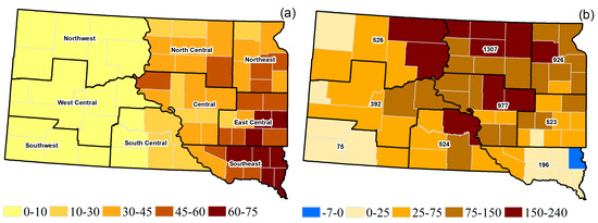
Figure 4.
(a) County-level stable cropland coverage in %, and (b) cropland net expansion in km2. The maps were overlaid with NASS reporting districts. Numbers on (b) present net cropland gains summarized by NASS districts.
Stable cropland areas were concentrated mostly in the eastern South Dakota where lands are more suitable for cultivation (Figure 4a), especially in the East-Central and Southeast NASS districts. Less than 10% of the western region was covered by stable croplands (Figure 4a). Between 2007 and 2015, cropland gains were mostly concentrated either in the northern or central South Dakota. Among the nine NASS reporting districts, North-Central, Central, and Northeast are the top three regions for cropland expansion with net gains of 1307 km2, 977 km2, and 926 km2, respectively (Figure 4b). There was less available cropland in the eastern South Dakota during the study period; thus, croplands expanded westward to neighboring counties, especially in the Northeast and South-Central districts (Figure 4b). Few gains in cropland were observed in the Southeast district, due to very limited land resources available for new cropland expansion (Figure 4a). There was also not much cropland expansion in Harding County (Figure 4b), located at the northwestern corner of the state, due to its dry and cold climate that does not support crop growth. The western side of the West Central and South West districts also showed little cropland expansion. These areas are mostly covered by lands unsuitable for cultivation (e.g., Black Hills National Forest, Badlands National Park, Buffalo Gap National Grassland). Of South Dakota’s 66 counties, Lincoln County in eastern South Dakota was the only one with a net loss in cropland area due to urban and suburban expansion of the Sioux Falls metropolitan area in northern Lincoln County (Figure 4b). Total population of the Sioux Falls metropolitan area grew from 132,358 to 171,530 (29.6%) between 2005 and 2015 [33].
In South Dakota, previous croplands are mostly concentrated on “prime” farmland, accounting for 75% of the total stable cropland area (Figure 5a). For more than 44,000 km2 of the stable cropland, only 3% cropland areas were in lands “unsuitable” for cultivation. However, between 2007 and 2015, farmers have been expanding croplands into more “fragile” and “unsuitable” lands to meet growing demand (48% of new expansion; Figure 5b). This trend indicates increasing scarcity of farm land: less area of prime cropland is available for cultivation.
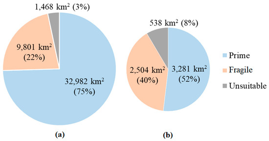
Figure 5.
Areas (km2) in (a) stable cropland and (b) converted cropland by Land Capability Class from the Soil Survey Geographic Database (SSURGO).
4. Discussion
4.1. Uncertainties in Land Cover/Land Use Dataset
A new land cover dataset for South Dakota was generated to characterize recent land cover/land use changes. In contrast to the CDL that went through several changes in methodology and input data, our product was generated more consistently to enable better change detection. One limitation of the new dataset is that the CDL was used as training dataset in a supervised classification process. Although the major commodity crops are mapped quite well in the CDL (generally, producer/use accuracies of above 95% for corn/soybean and approximate 90% for spring/winter wheat), accuracies of other classes can be low [20]. Thus, multiple steps were applied to reduce errors and uncertainties in the sample data. By using the CDL as the training dataset, we may magnify misclassifications found in CDL dataset. However, validation using the independent reference points showed comparable accuracy between LCLU maps from this study and the reclassified CDL (Table 1). Furthermore, our estimated cropland areas from our land cover maps are similar with those from the CDL and even closer to NASS statistics in the 2006-2009 period (Figure 3).
4.2. Characterizing Land Changes Using the Trajectory-Based Approach
Field-based estimations from the USDA are the most reliable data sources to quantify changes, but they offer limited spatial and/or temporal details. Therefore, researchers often turn into satellite-derived land cover/land use products with much higher spatiotemporal detail that allow depiction of both timing and location of land change. However, all satellite-based products suffer from misclassification errors that can falsely accentuate or attenuate changes between classes. To overcome this limitation, we developed a trajectory-based analysis that considers the entire land cover series to better determine land change at a particular location. The proposed approach stems from idea of examining a temporal array of “cropland” and “non-cropland” to determine land use status [13]. However, instead of looking at all possible combinations (211 = 2048 options) as demonstrated in [13], we modeled “cropland” and “non-cropland” time series as a binary array and described land use trajectory using logistic regression. This approach not only allows us to examine long time series but also to describe temporal land dynamics as a sigmoidal curve for a simple and consistent determination of land change. The results showed that cropland expansion estimated by the trajectory-based approach is much closer to the field-based reports from the USDA compared to the traditional bi-temporal change detection.
A key limitation of this study is low accuracy of the “non-cropland” classes (compare with Section 3.1); therefore, the analysis was focused only on cropland expansion since “cropland” is the most reliable class in our dataset (Table 1). Although, transitions in “cropland” can translate into changes in other classes, especially “grassland”, as published studies have shown that most of grassland losses are due to cropland expansion [2,3], the lower accuracy of “grassland” and “others” prevents exact quantification of their losses due to cropland expansion. In addition, our new dataset does not offer crop-specific categories like the CDL, preventing identification of the crops were planted on the newly cultivated lands.
5. Conclusions
Crop production plays critical role in South Dakota’s economy, especially commodity crops like corn/maize and soybean. However, losses of grassland and wetland area due to crop expansion may pose long-term risks to ecosystem services and biodiversity. Assessment of those risks requires accurate geospatial accounts of land change. This paper presented a comprehensive picture of LCLU transition in South Dakota between 2007 and 2015 using the fine spatiotemporal land cover dataset and the trajectory-based change detection approach. We found a net increase in cropland area of approximate 14% (5447 km2) in South Dakota. This result confirms substantial cropland expansion into grassland reported by previous studies [12,13,14]. Scarcity of land suitable for further cropland expansion was identified, pointing to the need for careful joint design and implementation of agriculture and energy policies to allow enable bioenergy demands to be met while protecting remaining wetlands and grasslands.
Supplementary Materials
The following are available online at https://www.mdpi.com/2073-445X/8/4/57/s1. Figure S1. Accuracy of county-level Random Forest models. Numbers are mean overall accuracies of 11 years, and color-coded background shows temporal coefficient of variation. Table S1. Fitted parameter coefficients, derived metrics from the Convex Quadratic (CxQ) model for land surface phenology [1]. Table S2. Pixel-wise comparison between predicted land cover maps (RFC) and the reclassified CDL for (a) 2006 and (b) 2012. PA is producer’s accuracy, UA is user’s accuracy. Overall accuracy appears in bold. Table S3. Correlation between estimated crop areas by this study (RFC), the reclassified CDL and the NASS statistics. Indication of significance: , *, and *** for p-values less than 0.05, 0.01, and 0.001, respectively.
Author Contributions
Conceptualization: L.H.N. and G.M.H.; Data curation: L.H.N. and D.R.J.; Analysis: L.H.N.; Writing—draft: L.H.N. and G.M.H.; Writing—review and editing: all authors.
Funding
This research was supported, in part, by NASA Land Cover Land Use Change program project NNX14AJ32G, the Geospatial Sciences Center of Excellence at South Dakota State University, and the Center for Global Change and Earth Observations at Michigan State University.
Acknowledgments
We would like to thank Dr. David E. Clay, Department of Agronomy, Horticulture & Plant Science, South Dakota State University for his comments on this article. We thank three anonymous reviewers for their useful feedback that helped us to improve the article’s clarity.
Conflicts of Interest
The authors declare no conflict of interest.
References
- Decision Innovation Solutions. 2014 South Dakota Agricultural Economic Contribution Study. Decision Innovation Solutions: Urbandale, IA 50322. Available online: https://sdda.sd.gov/office-of-the-secretary/publications/ (accessed on 15 December 2018).
- Wright, C.K.; Wimberly, M.C. Recent land use change in the Western Corn Belt threatens grasslands and wetlands. Proc. Natl. Acad. Sci. USA 2013, 110, 4134–4139. [Google Scholar] [CrossRef] [PubMed]
- Reitsma, K.D.; Clay, D.E.; Carlson, C.G.; Dunn, B.H.; Smart, A.J.; Wright, D.L.; Clay, S.A. Estimated South Dakota land use change from 2006 to 2012. iGrow Agronomy. 2014. Available online: https://igrow.org/up/resources/03-2001-2014.pdf (accessed on 15 December 2018).
- USDA-NASS (U.S. Department of Agriculture-National Agricultural Statistics Service). 2017 State Agriculture Overview: South Dakota. Available online: https://www.nass.usda.gov/Quick_Stats/Ag_Overview/stateOverview.php?state=SOUTH%20DAKOTA (accessed on 15 December 2018).
- Vaché, K.B.; Eilers, J.M.; Santelmann, M.V. Water quality modeling of alternative agricultural scenarios in the US Corn Belt. J. Am. Water Resour. Assoc. 2002, 38, 773–787. [Google Scholar] [CrossRef]
- Montgomery, D.R. Soil erosion and agricultural sustainability. Proc. Natl. Acad. Sci. USA 2007, 104, 13268–13272. [Google Scholar] [CrossRef] [PubMed]
- Stephens, S.E.; Walker, J.A.; Blunck, D.R.; Jayaraman, A.; Naugle, D.E.; Ringelman, J.K.; Smith, A.J. Predicting risk of habitat conversion in native temperate grasslands. Conserv. Biol. 2008, 22, 1320–1330. [Google Scholar] [CrossRef] [PubMed]
- Meehan, T.D.; Hurlbert, A.H.; Gratton, C. Bird communities in future bioenergy landscapes of the Upper Midwest. Proc. Natl. Acad. Sci. USA 2010, 107, 18533–18538. [Google Scholar] [CrossRef] [PubMed]
- Mutter, M.; Pavlacky, D.C.; Lanen, N.J.; Grenyer, R. Evaluating the impact of gas extraction infrastructure on the occupancy of sagebrush-obligate songbirds. Ecol. Appl. 2015, 25, 1175–1186. [Google Scholar] [CrossRef] [PubMed]
- Wimberly, M.C.; Narem, D.M.; Bauman, P.J.; Carlson, B.T.; Ahlering, M.A. Grassland connectivity in fragmented agricultural landscapes of the north-central United States. Biol. Conserv. 2018, 217, 121–130. [Google Scholar] [CrossRef]
- Faber, S.; Rundquist, S.; Male, T. Plowed Under: How Crop Subsidies Contribute to Massive Habitat Losses; Environmental Working Group: Washington, DC, USA, 2012. [Google Scholar]
- Decision Innovation Solutions. 2013 Multi-State Land Use Study: Estimated Land Use Changes 2007–2012. Urbandale, IA 50322: Decision Innovation Solutions. Available online: http://www.decision-innovation.com/spatial-time-series-analysis (accessed on 15 December 2018).
- Lark, T.J.; Salmon, J.M.; Gibbs, H.K. Cropland expansion outpaces agricultural and biofuel policies in the United States. Environ. Res. Lett. 2015, 10, 044003. [Google Scholar] [CrossRef]
- Arora, G.; Wolter, P.T. Tracking land cover change along the western edge of the US Corn Belt from 1984 through 2016 using satellite sensor data: Observed trends and contributing factors. J. Land Use Sci. 2018, 13, 59–80. [Google Scholar] [CrossRef]
- Nguyen, L.H.; Joshi, D.R.; Clay, D.E.; Henebry, G.M. Characterizing land cover/land use from multiple years of Landsat and MODIS time series: A novel approach using land surface phenology modeling and random forest classifiers. Remote Sens. Environ. 2018, 219. [Google Scholar] [CrossRef]
- De Beurs, K.M.; Henebry, G.M. Land surface phenology, climatic variation, and institutional change: Analyzing agricultural land cover change in Kazakhstan. Remote Sens. Environ. 2004, 89, 497–509. [Google Scholar] [CrossRef]
- Henebry, G.M.; de Beurs, K.M. Remote Sensing of Land Surface Phenology: A Prospectus. In Phenology: An Integrative Environmental Science, 2nd ed.; Schwartz, M.D., Ed.; Springer: New York, NY, USA, 2013; pp. 385–411. [Google Scholar]
- NASA LP DAAC, 2006, MODIS Terra/Aqua Land Surface Temperature/Emissivity 8-Day L3 Global 1 km SIN Grid. Version 5. NASA EOSDIS Land Processes DAAC, USGS Earth Resources Observation and Science (EROS) Center, Sioux Falls, South Dakota. Available online: https://lpdaac.usgs.gov (accessed on 15 January 2017).
- Wan, Z. New refinements and validation of the MODIS land-surface temperature/emissivity products. Remote Sens. Environ. 2008, 112, 59–74. [Google Scholar] [CrossRef]
- Boryan, C.; Yang, Z.; Mueller, R.; Craig, M. Monitoring US agriculture: The US Department of Agriculture, National Agricultural Statistics Service, Cropland Data Layer program. Geocarto Int. 2011, 26, 341–358. [Google Scholar] [CrossRef]
- Reitsma, K.D.; Clay, D.E.; Clay, S.A.; Dunn, B.H.; Reese, C. Does the US cropland data layer provide an accurate benchmark for land-use change estimates? Agron. J. 2016, 108, 266–272. [Google Scholar] [CrossRef]
- Lark, T.J.; Mueller, R.M.; Johnson, D.M.; Gibbs, H.K. Measuring land-use and land-cover change using the US department of agriculture’s cropland data layer: Cautions and recommendations. Int. J. Appl. Earth Obs. Geoinf. 2017, 62, 224–235. [Google Scholar] [CrossRef]
- Zhang, H.K.; Roy, D.P. Using the 500 m MODIS land cover product to derive a consistent continental scale 30 m Landsat land cover classification. Remote Sens. Environ. 2017, 197, 15–34. [Google Scholar] [CrossRef]
- Loveland, T.R.; Cochrane, M.A.; Henebry, G.M. Landsat still contributing to environmental research. Trends Ecol. Evol. 2008, 23, 182–183. [Google Scholar] [CrossRef] [PubMed]
- USDA-NRCS (U.S. Department of Agriculture-Natural Resources Conservation Service). 2018. Soil Survey Geographic (SSURGO) Database. Available online: https://nrcs.app.box.com/v/soils (accessed on 5 October 2018).
- United States Department of Agriculture (USDA). 2017 Quick Stats 2.0. U.S. Department of Agriculture, National Agricultural Statistics Service, Washington DC. Available online: https://quickstats.nass.usda.gov/ (accessed on 21 December 2018).
- 2007 Census of Agriculture: South Dakota State and County Data. U.S. Department of Agriculture, National Agricultural Statistics Service. 2009. Available online: https://www.nass.usda.gov/AgCensus/ (accessed on 10 March 2019).
- 2012 Census of Agriculture: South Dakota State and County Data. U.S. Department of Agriculture, National Agricultural Statistics Service. 2014. Available online: https://www.nass.usda.gov/AgCensus/ (accessed on 10 March 2019).
- U.S. Department of Agriculture. Summary Report: 2007 National Resources Inventory; Natural Resources Conservation Service: Washington, DC, USA; Center for Survey Statistics and Methodology, Iowa State University: Ames, IA, USA, 2009. Available online: http://www.nrcs.usda.gov/Internet/FSE_DOCUMENTS/stelprdb1167354.pdf (accessed on 10 March 2019).
- U.S. Department of Agriculture. Summary Report: 2010 National Resources Inventory; Natural Resources Conservation Service: Washington, DC, USA; Center for Survey Statistics and Methodology, Iowa State University: Ames, IA, USA, 2013. Available online: http://www.nrcs.usda.gov/technical/NRI/2007/2007_NRI_Summary.pdf (accessed on 10 March 2019).
- U.S. Department of Agriculture. Summary Report: 2012 National Resources Inventory; Natural Resources Conservation Service: Washington, DC, USA; Center for Survey Statistics and Methodology, Iowa State University: Ames, IA, USA, 2015. Available online: http://www.nrcs.usda.gov/technical/nri/15summary (accessed on 10 March 2019).
- U.S. Department of Agriculture. Summary Report: 2015 National Resources Inventory; Natural Resources Conservation Service: Washington, DC, USA; Center for Survey Statistics and Methodology, Iowa State University: Ames, IA, USA, 2018. Available online: http://www.nrcs.usda.gov/technical/nri/15summary (accessed on 10 March 2019).
- U.S. Census Bureau, American Community Survey-ACS. ACS 5-Year estimates of Total Population for Sioux Falls city, SD; generated by Lan Nguyen; using American FactFinder. Available online: http://factfinder.census.gov (accessed on 15 December 2018).
© 2019 by the authors. Licensee MDPI, Basel, Switzerland. This article is an open access article distributed under the terms and conditions of the Creative Commons Attribution (CC BY) license (http://creativecommons.org/licenses/by/4.0/).