
Identifying Employment Subcenters: The Method of Exponentially Declining Cutoffs


Abstract
:1. Introduction
2. Identifying Employment Subcenters
The Method of Exponentially Declining Cutoffs
3. The Method of Exponentially Declining Cutoffs
| D | employment density |
| E | total employment |
| α | cutoff gradient |
| x | (Euclidean) distance from the metropolitan center |
| z | zonal index |
| set of candidate zones | |
| set of candidate subcenters |
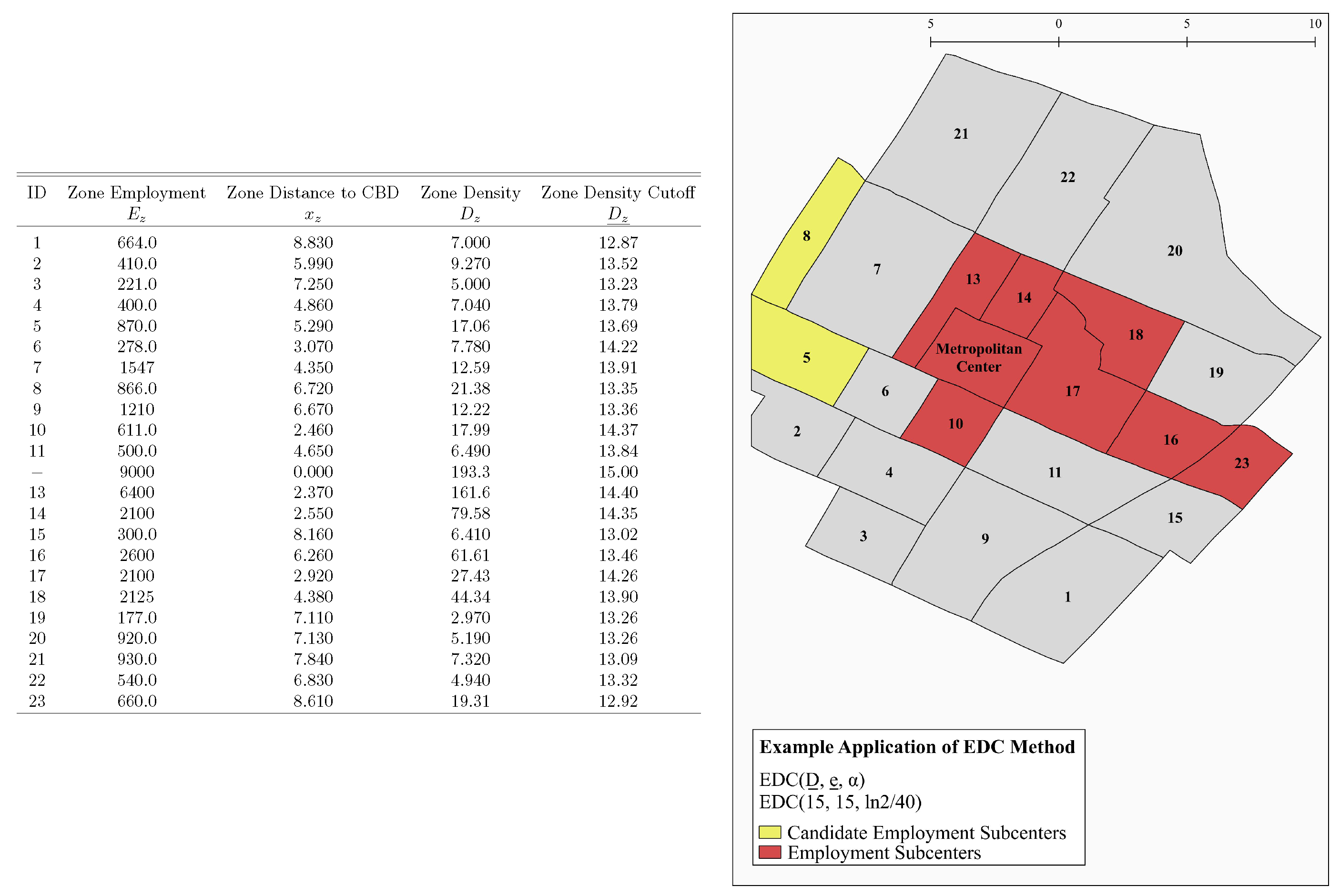
- Determine the cutoff level of employment density for each zone.where is the cutoff employment density in zone z, is the cutoff employment density at the metropolitan center, is the distance between the zone centroid and the metropolitan center and α is the cutoff gradient, the proportional rate of decline of the cutoff with distance (e.g., 20% per kilometer). In other words, the cutoff employment density in zone z equals the cutoff employment density at the metropolitan center, adjusted downward as a function of distance from the metropolitan center according to .
- Determine the set of candidate zones.A candidate zone is a zone whose actual employment density, , exceeds the cutoff employment density for that zone. Denoting by the set of candidate zones,In other words, a zone is a candidate zone if and only if its employment density exceeds its cutoff employment density based on distance from the metropolitan center.
- Group zones into candidate subcenters.A candidate subcenter is a set of candidate zones that form a contiguous set and are contiguous to no other candidate zones. By definition, candidate subcenters are mutually exclusive (i.e., a candidate zone cannot be in more than one candidate subcenter). Let s index the candidate subcenters and denote the set of candidate subcenters. By definition .
- Determine the cutoff level of total employment for each candidate subcenter.where is cutoff total employment in candidate subcenter s, is cutoff total employment at the metropolitan center and is the employment-weighted distance between the candidate subcenter and the metropolitan center. In particular, where n is the number of zones in candidate subcenter s, () is the distance between zone z and the metropolitan center, and is the total employment of zone z, is defined as . In other words, the cutoff level of total employment for a candidate subcenter equals the cutoff level of total employment for a subcenter at the metropolitan center, adjusted downward as a function of the distance from the employment-weighted centroid of the candidate subcenter to the metropolitan center according to .
- Determine the set of subcenters.Where S is the set of (proper) subcenters and is the total employment of candidate subcenter s,In other words, a candidate subcenter is a (proper) subcenter if and only if its total employment exceeds its total employment cutoff based on distance from the metropolitan center.
4. A Refinement of the Procedure
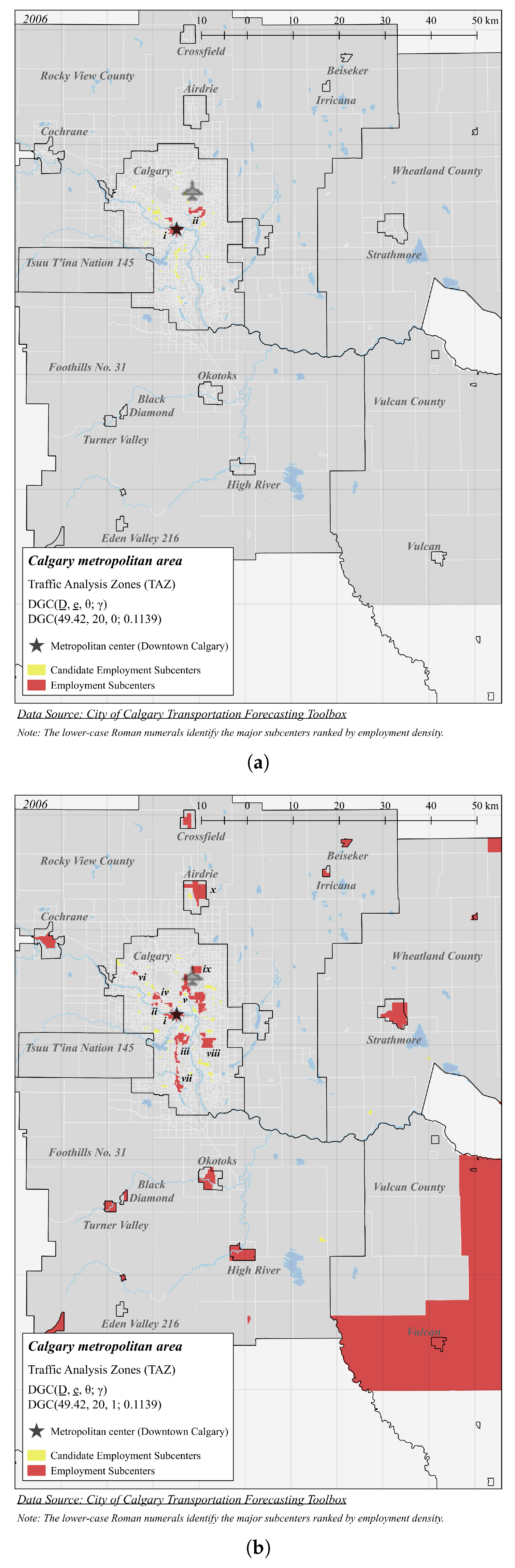
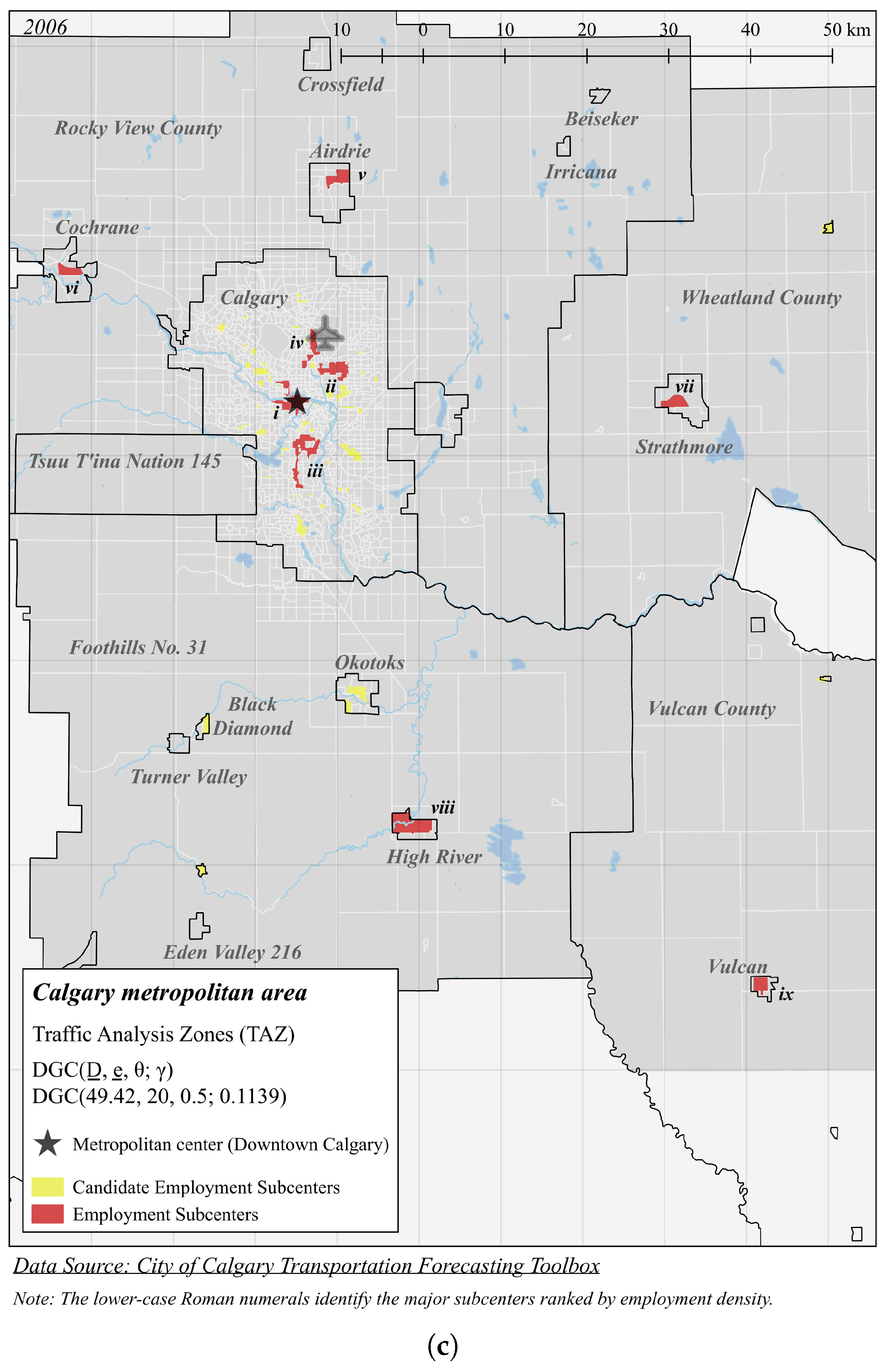
4.1. Calgary
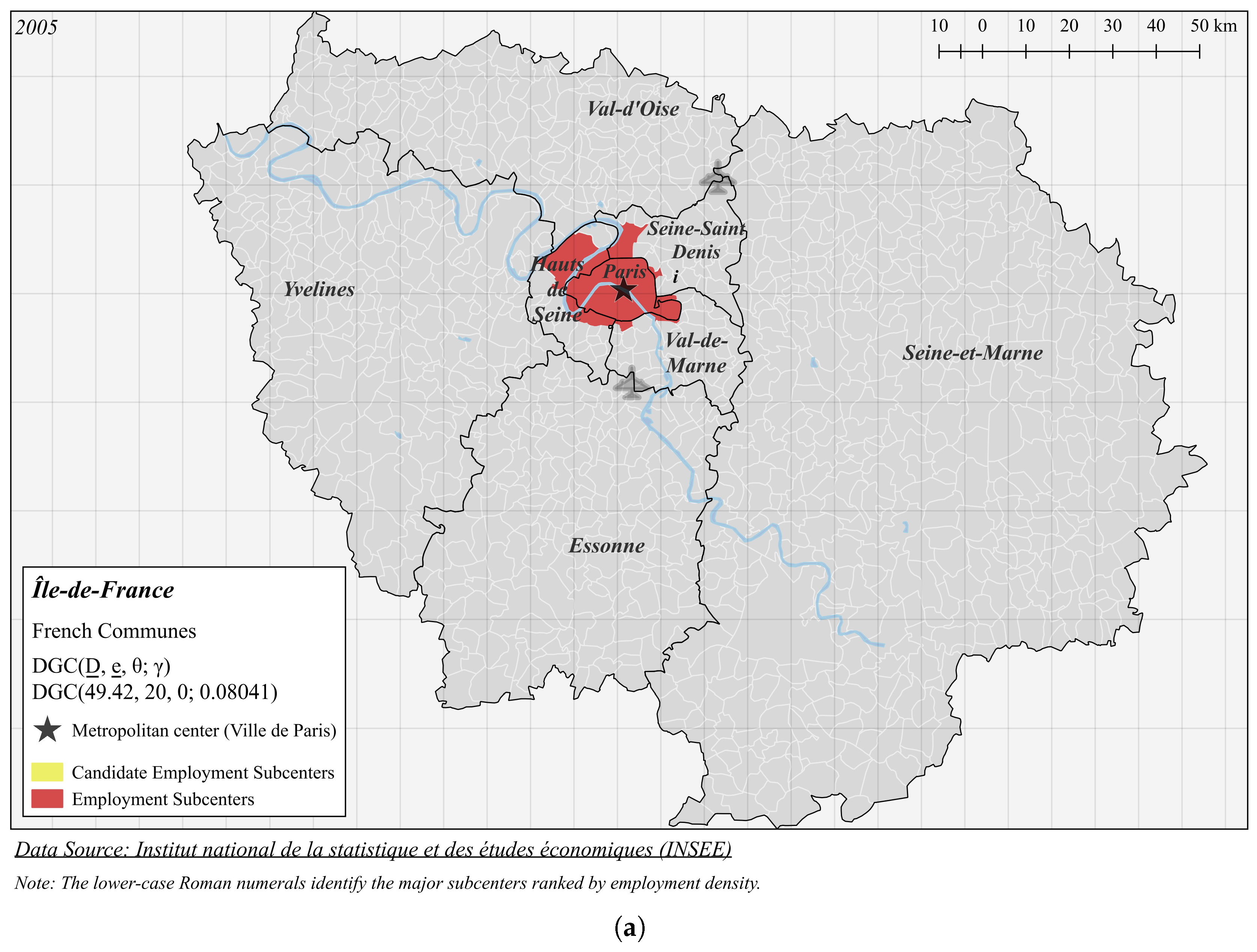
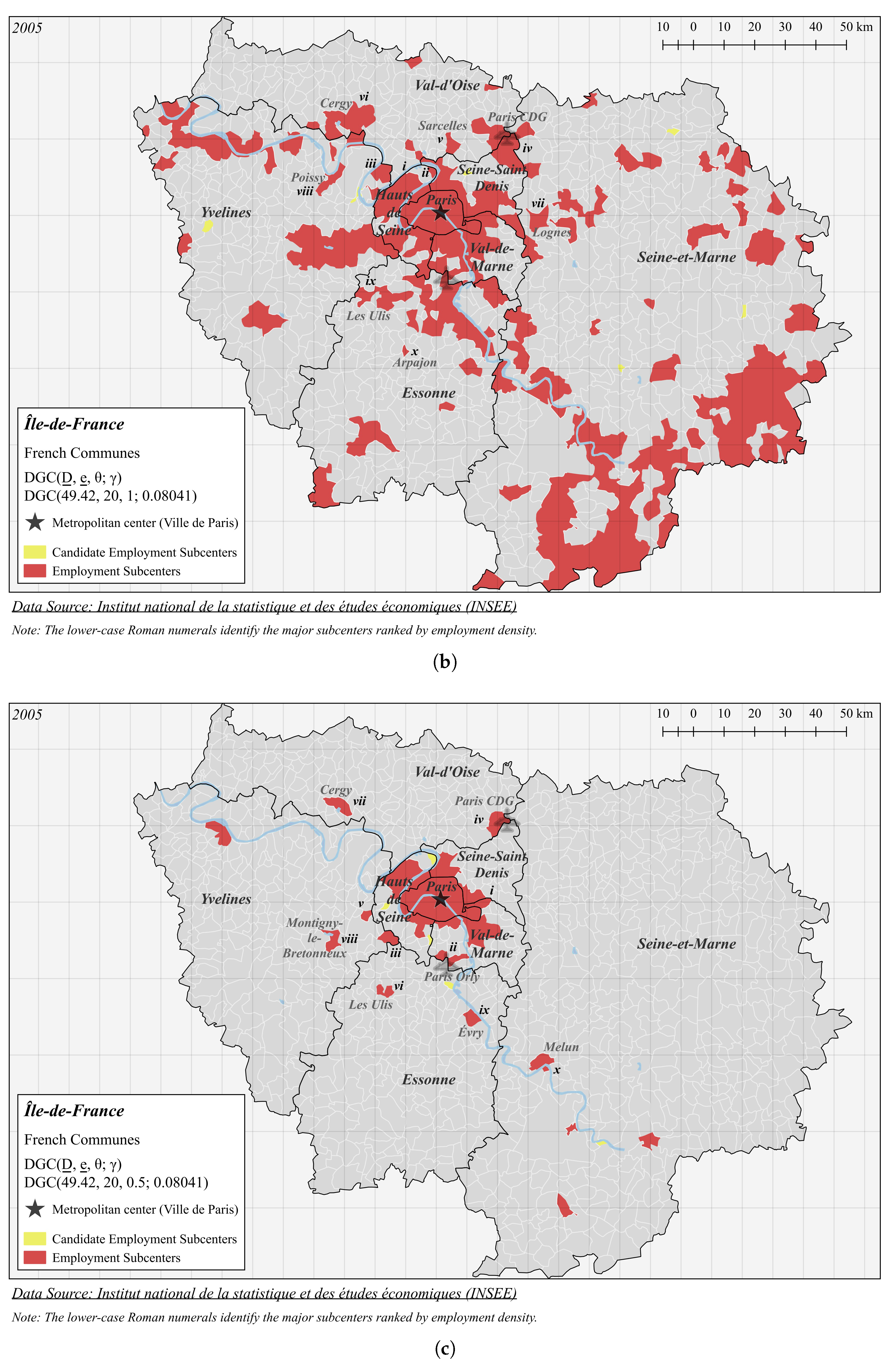
4.2. Paris
5. Discussion
5.1. Technical Issues
5.2. Extensions and Applications
6. Concluding Comments
Acknowledgments
Author Contributions
Conflicts of Interest
Appendix A.

| Statistic | N | Mean | Median | SD | Min | Max | Units |
|---|---|---|---|---|---|---|---|
| Panel A: Los Angeles Metropolitan Area (TAZ). | |||||||
| Employment | 3999 | 1870 | 949.0 | 2828 | 0 | 45,295 | |
| Density | 3999 | 15.31 | 6.281 | 56.39 | 0.000 | 2107 | employees/hectare |
| Area | 3999 | 2202 | 167.6 | 23,455 | 10.54 | 717,928 | hectares |
| Distance to CBD | 3999 | 57.88 | 44.70 | 47.68 | 0.000 | 381.4 | kilometers |
| Panel B: Calgary Metropolitan Area (TAZ). | |||||||
| Employment | 1869 | 355.4 | 88.00 | 923.3 | 0.000 | 16,236 | |
| Density | 1869 | 19.47 | 1.235 | 118.1 | 0.000 | 2823 | employees/hectare |
| Area | 1869 | 740.0 | 65.56 | 3000 | 0.230 | 73,478 | hectares |
| Distance to CBD | 1869 | 16.00 | 12.30 | 14.22 | 0.000 | 100.4 | kilometers |
| Panel C: Paris metropolitan area (Communes). | |||||||
| Employment | 1299 | 4126 | 358.0 | 13,354 | 5.000 | 200,697 | |
| Density | 1299 | 8.974 | 0.4420 | 38.97 | 0.009400 | 632.2 | employees/hectare |
| Area | 1299 | 929.1 | 765.7 | 775.2 | 7.977 | 17,205 | hectares |
| Distance to CBD | 1299 | 41.14 | 39.76 | 20.60 | 0.000 | 92.57 | kilometers |
| ID | Density | Employment | Area | Distance to CBD | # Zones |
|---|---|---|---|---|---|
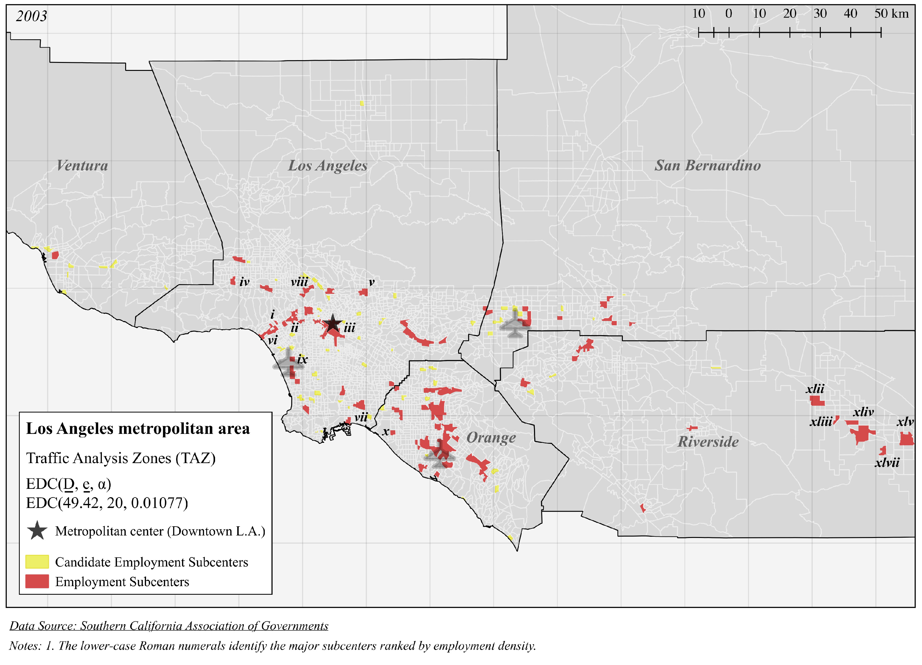
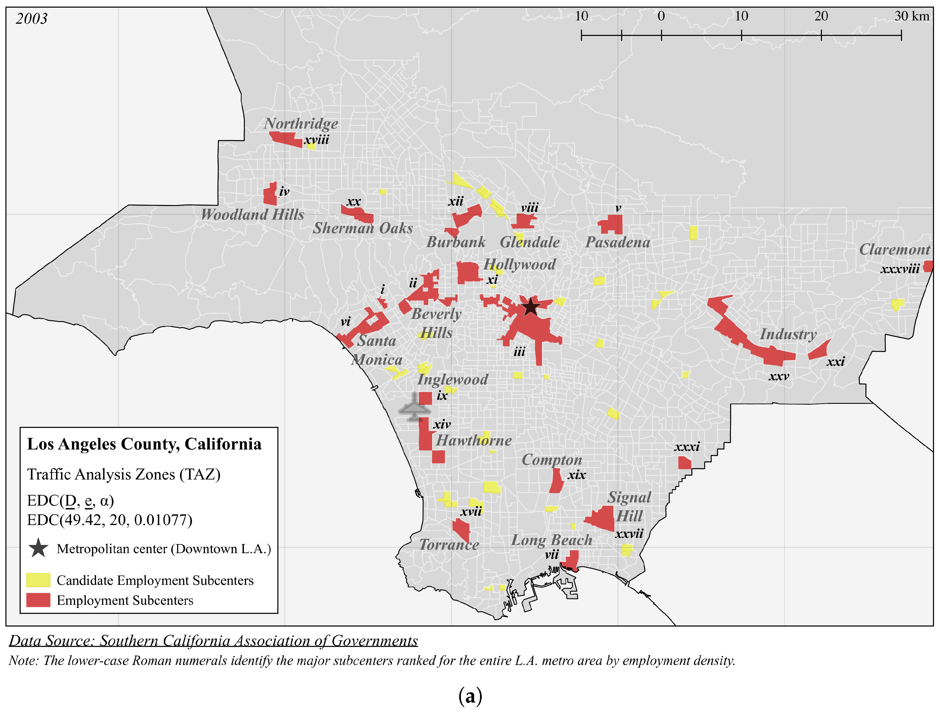
| Panel A (Figure 3): EDC(49.42, 20, 0.01077) | |||||
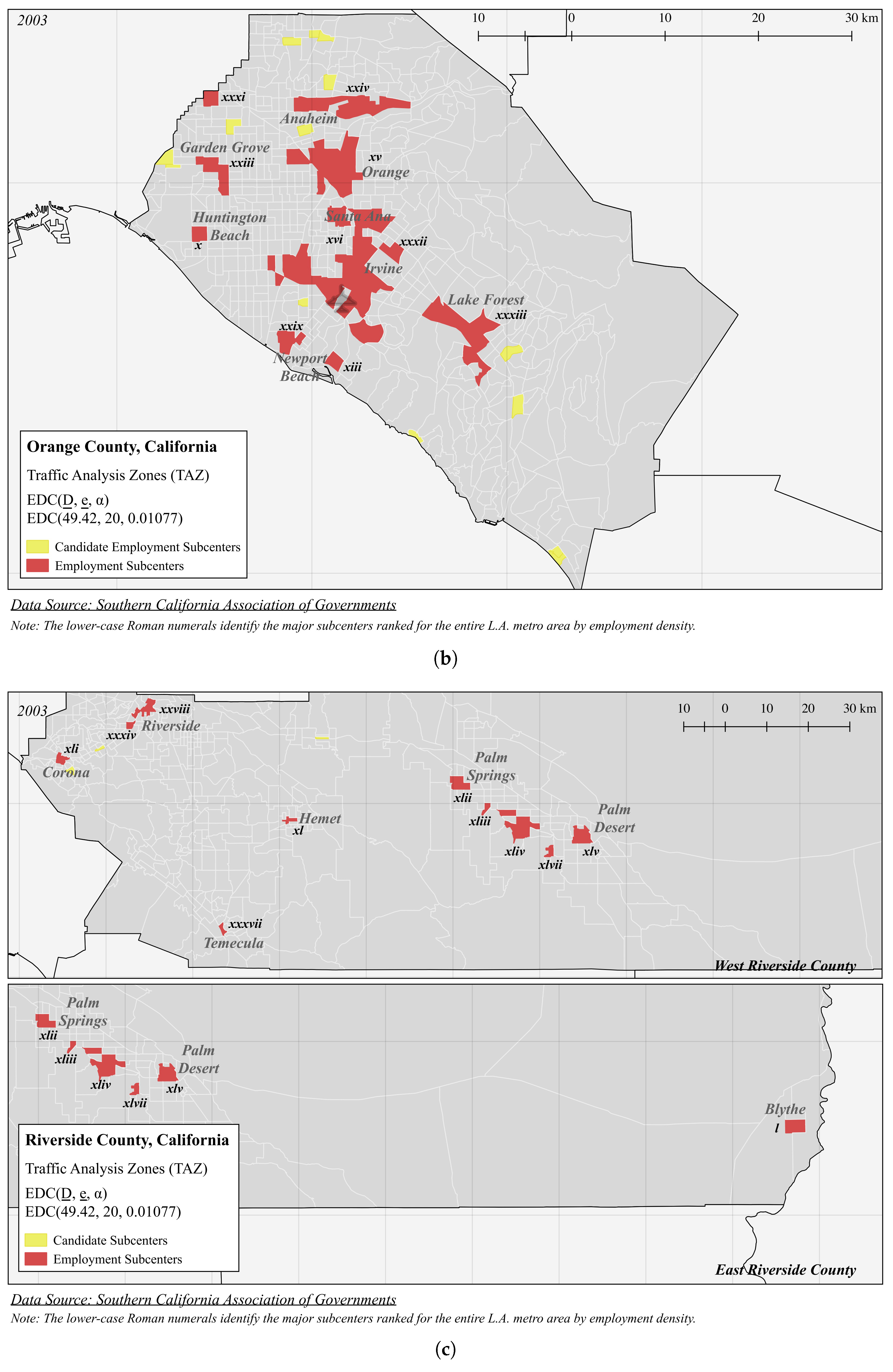
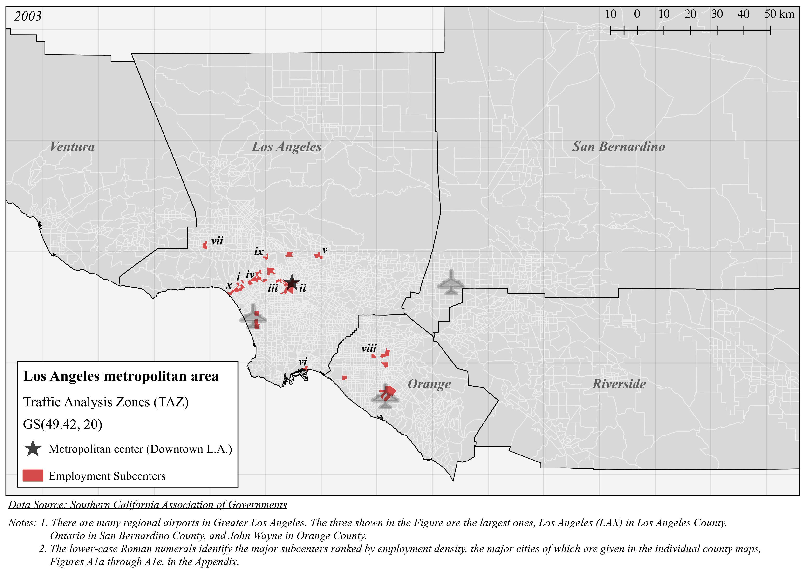
| i | 489.4 | 47,463 | 96.98 | 0.2660 | 4 |
| ii | 125.8 | 149,665 | 1189 | 4.964 | 19 |
| iii | 123.3 | 378,392 | 3067 | 17.75 | 58 |
| iv | 118.0 | 45,609 | 386.4 | 19.19 | 4 |
| v | 103.1 | 60,041 | 582.6 | 29.88 | 6 |
| vi | 98.59 | 99,894 | 1013 | 4.296 | 14 |
| vii | 96.23 | 37,892 | 393.8 | 40.20 | 5 |
| viii | 87.69 | 35,234 | 401.8 | 20.30 | 6 |
| ix | 80.86 | 20,890 | 258.4 | 13.32 | 2 |
| x | 78.80 | 20,425 | 261.6 | 52.61 | 1 |
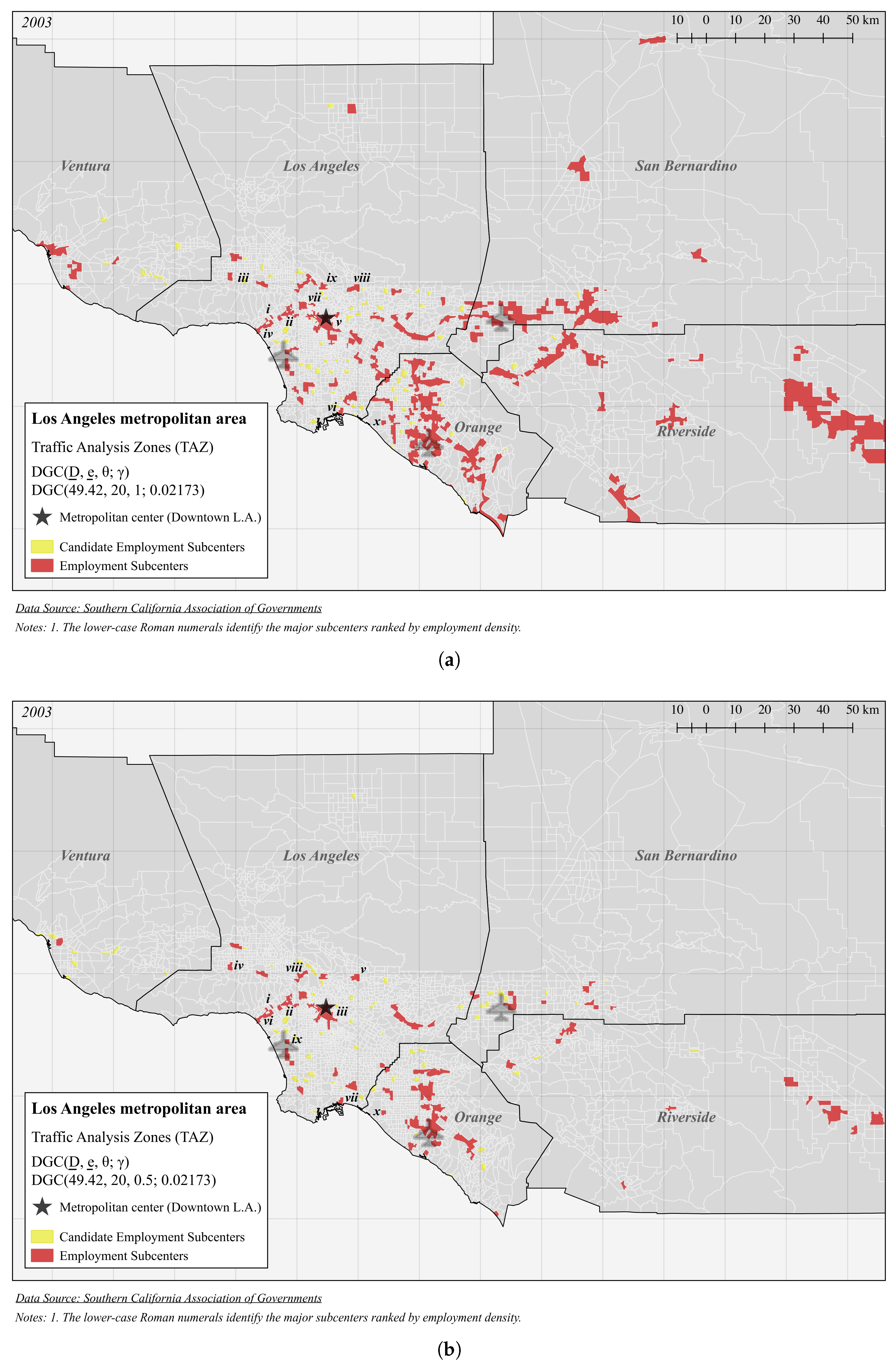
| Panel B (Figure 4a): DGC(49.42, 20, 1; 0.02173) | |||||
| i | 489.4 | 47,463 | 96.98 | 0.2660 | 4 |
| ii | 121.9 | 152,216 | 1249 | 5.007 | 20 |
| iii | 107.5 | 47,423 | 441.1 | 19.23 | 5 |
| iv | 98.59 | 99,894 | 1013 | 4.296 | 14 |
| v | 98.37 | 439,633 | 4469 | 18.13 | 80 |
| vi | 96.23 | 37,892 | 393.8 | 40.20 | 5 |
| vii | 96.01 | 14,576 | 151.8 | 14.65 | 3 |
| viii | 85.36 | 65,090 | 762.6 | 29.73 | 7 |
| ix | 82.77 | 36,697 | 443.4 | 20.30 | 7 |
| x | 78.08 | 20,425 | 261.6 | 52.61 | 1 |
| Panel C (Figure 4b): DGC(49.42, 20, 0.5; 0.02173) | |||||
| i | 489.4 | 47,463 | 96.98 | 0.2660 | 4 |
| ii | 125.8 | 149,665 | 1189 | 4.964 | 19 |
| iii | 123.3 | 378,392 | 3067 | 17.75 | 58 |
| iv | 118.0 | 45,609 | 386.4 | 19.19 | 4 |
| v | 103.1 | 60,041 | 582.6 | 29.88 | 6 |
| vi | 98.59 | 99,894 | 1013 | 4.296 | 14 |
| vii | 96.23 | 37,892 | 393.8 | 40.20 | 5 |
| viii | 87.69 | 35,234 | 401.8 | 20.30 | 6 |
| ix | 80.86 | 20,890 | 258.4 | 13.32 | 2 |
| x | 78.08 | 20,425 | 261.6 | 52.61 | 1 |
| ID | Density | Employment | Area | Distance to CBD | # Zones |
|---|---|---|---|---|---|
| Panel A (Figure 5a): DGC(49.42, 20, 0; 0.1139) | |||||
| i | 274.2 | 164,787 | 601.0 | 0.6860 | 46 |
| ii | 74.13 | 25,006 | 337.3 | 6.225 | 15 |
| Panel B (Figure 5b): DGC(49.42, 20, 1; 0.1139) | |||||
| i | 244.1 | 169,117 | 692.8 | 0.7170 | 50 |
| ii | 192.2 | 12,161 | 63.28 | 5.064 | 2 |
| iii | 60.15 | 43,042 | 715.5 | 6.691 | 30 |
| iv | 58.26 | 13,155 | 225.8 | 5.776 | 4 |
| v | 49.07 | 63,340 | 1290 | 6.173 | 48 |
| vi | 46.83 | 4734 | 101.1 | 12.90 | 5 |
| vii | 28.60 | 11,121 | 388.9 | 14.97 | 17 |
| viii | 27.47 | 16,589 | 604.0 | 8.898 | 12 |
| ix | 21.44 | 6606 | 308.2 | 10.67 | 1 |
| x | 7.346 | 8999 | 1225 | 27.62 | 8 |
| Panel C (Figure 5c): DGC(49.42, 20, 0.5; 0.1139) | |||||
| i | 255.6 | 167,386 | 654.9 | 0.7080 | 48 |
| ii | 65.24 | 29,712 | 455.5 | 6.258 | 20 |
| iii | 62.67 | 41,328 | 659.4 | 6.713 | 28 |
| iv | 43.81 | 13,751 | 313.9 | 6.647 | 8 |
| v | 14.09 | 5530 | 392.6 | 27.84 | 2 |
| vi | 11.49 | 3271 | 284.7 | 31.98 | 2 |
| vii | 10.91 | 3856 | 353.5 | 46.06 | 1 |
| viii | 0.116 | 6098 | 997.0 | 53.64 | 3 |
| ix | 3.610 | 985 | 272.9 | 90.92 | 2 |
| x | 1.739 | 343 | 197.2 | 76.10 | 1 |
| ID | Density | Employment | Area | Distance to CBD | # Zones |
|---|---|---|---|---|---|
| Panel A (Figure 6a): DGC(49.42, 20, 0; 0.08041) | |||||
| i | 126.5 | 2,502,365 | 19,775 | 4.665 | 46 |
| Panel B (Figure 6b): DGC(49.42, 20, 1; 0.08041) | |||||
| i | 48.05 | 3,649,419 | 75,957 | 7.871 | 137 |
| ii | 44.22 | 12,731 | 287.9 | 7.771 | 1 |
| iii | 19.09 | 24,442 | 1280 | 14.08 | 2 |
| iv | 19.06 | 146,555 | 7690 | 19.74 | 6 |
| v | 18.29 | 15,358 | 839.6 | 13.88 | 1 |
| vi | 14.79 | 90,421 | 6115 | 26.79 | 7 |
| vii | 14.26 | 20,729 | 1453 | 21.71 | 3 |
| viii | 14.04 | 17,870 | 1273 | 23.84 | 1 |
| ix | 14.02 | 45.021 | 3211 | 22.84 | 4 |
| x | 9.684 | 2516 | 259.8 | 31.76 | 1 |
| Panel C (Figure 6c): DGC(49.42, 20, 0.5; 0.08041) | |||||
| i | 104.4 | 2,746,070 | 26,302 | 5.088 | 57 |
| ii | 39.11 | 41,596 | 1063 | 14.01 | 2 |
| iii | 35.48 | 31,950 | 900.5 | 14.20 | 1 |
| iv | 30.45 | 44,650 | 1466 | 19.82 | 1 |
| v | 29.50 | 12,525 | 424.6 | 16.26 | 1 |
| vi | 25.69 | 14,479 | 563.7 | 23.81 | 1 |
| vii | 24.33 | 34,849 | 1432 | 28.66 | 1 |
| viii | 23.13 | 24,568 | 1062 | 24.95 | 1 |
| ix | 18.15 | 15,445 | 851.0 | 27.54 | 1 |
| x | 14.85 | 20,380 | 1372 | 42.59 | 2 |
Appendix B. Subcenter Identification Algorithm (R Script)
############################################################################################
#####################################################################################
#####  SUBCENTER IDENTIFICATION ALGORITHM companion to:
####  Ban, Arnott, Macdonald
###   "Identifying Employment Subcenters: The Method of Exponentially
##   Declining Cutoffs"
#
#
# R Code which reads in a shapefile of a metropolitan area with employment data for each
# geography (i.e. Census Tract; TAZ). This data is used in identifying employment subcenters
# based on the accompanying paper’s Density Gradient Cutoff (DGC) methodology. Special cases
# of this function determine subcenters based on the Giuliano--Small (GS) or Exponentially
# Declining Cutoff (EDC) methodologies.
#
# INPUTS:
# [shapefile] -- SpatialPolygonsDataFrame
#  ".shp" file of metropolitan area with employment by zone
# [output]  -- character (default: working directory)
#  Output folder location where to save files
# [employment] -- character
#  Name of the employment variable
# [location] -- character (vector)
#  Vector of the names of ID, County, or Location variables that should be kept with the
#  shapefile (additional variables are then deleted)
# [D]     -- numeric
#  User specified cutoff employment density threshold at metropolitan center.
#  Should be specified in the same units as the algorithm (if units=="metric" then D
#  should be specified as employees/hectare; if units=="imperial" then D should be
#  specified as employees/acre)
# [E]     -- numeric
#  User specified cutoff total employment threshold at metropolitan center.
# [type]   -- ("DGC" (default) or "EDC")
#  If =="EDC" then employs the method of Exponentially Declining Cutoff (EDC)
#  If =="DGC" then employs the method of Density Gradient Cutoff (DGC)
# [alpha]   -- numeric (default: ln2/40)
#  Used only under the "EDC" method. User specified value of the cutoff gradient.
# [theta]   -- numeric in [0,1]
#  Weight used in absolute and relative density and employment cutoffs (theta==0 => all
#  weight on absolute density; equivalent to G.S. methodology)
# [gamma]   -- numeric (optional)
#  Used only under the "DGC" method and can be manually specified.
#  Default calculates employment density gradient estimated by: ln(D_z) = c - gamma∗x_z
#  Where "D" and "x" are zone level employment densities and distance to CBD.
# [units]   -- ("metric" (default) or "imperial")
#  If "metric" then analysis is done with distance in kilometers and area in hectares.
#  If "imperial then analysis done with distance in miles and area in acres.
# [generate] -- TRUE | FALSE (default: TRUE)
#  Set to FALSE if the output files should not be saved - subcenter results will only be
#  available in the R environment.
#
# OUTPUTS:
# subcenters[[1]]
#  ".shp" file with variable "subcenter" which identifies candidate subcenters (= 1)
#  and full subcenters (= 2)
# subcenters[[2]]
#  ".csv" file labeling each subcenter starting from the highest subcenter density
#  with respective employment, area, density and zone information.
# subcenters[[3]]
#  Value of the density cutoff gradient ([alpha] or [gamma]).

x <- c("sp", "spdep", "rgdal", "geosphere", "rgeos", "maptools")
uninstalled <- x[!(x %in% installed.packages()[,"Package"])]
if(length(uninstalled)) install.packages(uninstalled)
lapply(x, library, character.only = TRUE)
rm(x, uninstalled)

############################################################################################
############################################################################################
subcenters <- function(shapefile, output=getwd(), employment, location, type="DGC", D, E,
 alpha, theta, gamma=NULL, units="metric", generate=TRUE){

SESSION <- paste0(unlist(strsplit(as.character(Sys.Date()), "[-]"))[[3]],
 paste0(unlist(strsplit(as.character(Sys.Date()), "[-]"))[[2]],
 substr(unlist(strsplit(as.character(Sys.Date()), "[-]"))[[1]], 3, 4)))

# RETREIVE INTERNAL POLYGON ID
shapefile@data$IDpg <- as.factor(sapply(slot(shapefile, "polygons"),
 function(x) slot(x, "ID")))

# CHANGE THE NAME OF THE VARIABLE THE USER IDENTIFIES AS EMPLOYMENT
names(shapefile@data)[names(shapefile@data)==employment] <- "employment"

shapefile@data$area <- rep(0, length(shapefile@data[,1]))
for(i in 1:length(shapefile@data[,1])){
 shapefile@data$area[i] <- areaPolygon(lapply(slot(shapefile, "polygons"),
  function(x) lapply(slot(x, "Polygons"),
  function(y) slot(y, "coords")))[[i]][[1]])
}

if(units=="metric"){
 shapefile@data$area <- shapefile@data$area∗0.0001
} else if(units=="imperial"){
 shapefile@data$area <- shapefile@data$area∗0.000247105
} else {
 shapefile@data$area <- NA
}

# CALCULATE EMPLOYMENT DENSITY USED TO DETERMINE THE CBD
shapefile@data$density <- shapefile@data$employment/shapefile@data$area
shapefile@data$density <- ifelse(is.na(shapefile@data$density), 0, shapefile@data$density)

# CBD IS DEFINED AS THE CENSUS TRACT WITH THE MAXIMUM EMPLOYMENT DENSITY
# DISTANCE IS CALCULATED BETWEEN CENSUS CENTROIDS AND CALCULATED IN MILES
shapefile@data$distance <- 3963.0∗acos(sin(coordinates(shapefile[shapefile@data$density==
 max(shapefile@data$density),])[2]/57.2958)∗sin(coordinates(shapefile)[,2]/57.2958) +
 cos(coordinates(shapefile[shapefile@data$density==
 max(shapefile@data$density),])[2]/57.2958)∗cos(coordinates(shapefile)[,2]/57.2958)∗
 cos(coordinates(shapefile)[,1]/57.2958 -
 coordinates(shapefile[shapefile@data$density==max(shapefile@data$density),])[1]/57.2958))

if(units=="metric"){
 shapefile@data$distance <- shapefile@data$distance∗1.60934
} else if(units=="imperial"){
 shapefile@data$distance <- shapefile@data$distance
} else {
 shapefile@data$distance <- NA
}

# GAMMA IS EITHER LOG(2)/40 IN THE NEG. EXPONENTIAL MODEL OR THE EMPLOYMENT GRADIENT IN DGC
# MODELS
 if(type=="EDC") {
  gradient <- alpha
  theta <- 1
 } else if(type=="DGC" & !is.null(gamma)) {
  gradient <- gamma
 } else if(type=="DGC" & is.null(gamma)) {
  gradient <- abs(as.numeric(as.character(lm(log(ifelse(shapefile@data$density > 0,
   shapefile@data$density, 0.5)) ~ shapefile@data$distance)$coefficients[2])))
 }

# KEEP ONLY THE VARIABLES NEEDED FOR SC IDENTIFICATION AND IMPORTANT LOCATION AND
# IDENTIFYING VARIABLES
 keeps <- c("IDpg", "employment","area", "distance", "density", location)
 shapefile <- shapefile[ , (colnames(shapefile@data) %in% keeps)]
 rm(keeps)

 shapefile@data$longitude <- coordinates(shapefile)[,1]
 shapefile@data$latitude <- coordinates(shapefile)[,2]

# FOR EACH INDIVIDUAL CENSUS TRACT DETERMINE WHETHER THE DENSITY MEETS THE EXPONENTIALLY
# DECREASING DENSITY THRESHOLD. IF YES THEN IT CAN BE CONSIDERED A CANDIDATE SUBCENTER (==1)
 shapefile@data$Dcutoff <- D∗exp(-theta∗gradient∗shapefile@data$distance)
 shapefile@data$subcenter <- ifelse(shapefile@data$density > shapefile@data$Dcutoff, 1, 0)

# THE TOTAL EMPLOYMENT CUTOFF MUST BE APPLIED TO CONTIGUOUS TRACTS OF CANDIDATE SUBCENTERS
# TO IDENTIFY CONTIGUOUS TRACTS, WE FIRST DEFINE THE ADJACENCY MATRIX WHICH DETERMINES WHAT
# CENSUS TRACTS ARE ADJACENT TO EACH OTHER AND FURTHER DEFINES ALL CONTIGUOUS BLOCKS OF
# CANDIDATE SUBCENTERS.
 candidates <- shapefile[shapefile@data$subcenter==1,]
 adjacency <- gTouches(candidates, returnDense=TRUE, byid=TRUE)
 adjacency[adjacency == FALSE] <- 0
 adjacency[adjacency ==TRUE] <- 1

 colnames(adjacency) <- rownames(adjacency)
 n = nrow(adjacency)
 amat <- matrix(0,nrow=n,ncol=n)
 amat[row(amat)==col(amat)] <- 1
 colnames(amat) <- colnames(adjacency)
 rownames(amat) <- rownames(adjacency)
 bmat <- adjacency
 wmat1 <- adjacency
 newnum = sum(bmat)
 cnt = 1
 while (newnum > 0) {
  amat <- amat+bmat
  wmat2 <- wmat1%∗%adjacency
  bmat <- ifelse(wmat2 > 0 & amat==0, 1, 0)
  wmat1 <- wmat2
  newnum = sum(bmat)
  cnt = cnt+1
 }

 Ez <- amat%∗%diag(candidates@data$employment)
 Xz <- amat%∗%diag(candidates@data$distance)
 Az <- amat%∗%diag(candidates@data$area)
 EzXz <- Ez∗Xz

 IDz <- amat∗as.numeric(colnames(amat))
 IDz[IDz==0] <- 999999999999999999
 IDz <- apply(cbind(apply(IDz, 1, min), apply(IDz, 2, min)), 1, min)

# FOR EACH CANDIDATE SUBCENTER WE CALCULATE THE TOTAL EMPLOYMENT, DISTANCE WEIGHTED
# EMPLOYMENT AND AREA FROM THE RESPECTIVE BROADER CONTIGUOUS GROUP OF SUBCENTERS.
 candidates@data$SCemployment <- rowSums(Ez, na.rm = FALSE, dims = 1)
 candidates@data$SCdistance <- rowSums(EzXz, na.rm = FALSE, dims = 1)/candidates@data$SCemployment
 candidates@data$SCarea <- rowSums(Az, na.rm = FALSE, dims = 1)
 candidates@data$SCdensity <- candidates@data$SCemployment/candidates@data$SCarea

# EACH CANDIDATE SUBSCENTER IS COMPARED AGAINSED THE TOTAL EMPLOYMENT CUTOFF FOR THE BROADER
# GROUP OF CONTIGUOUS TRACTS.
 candidates@data$Ecutoff <- E∗exp(-theta∗gradient∗candidates@data$SCdistance)
 candidates@data$subcenter <- ifelse(candidates@data$SCemployment > candidates@data$Ecutoff,
  candidates@data$subcenter + 1, candidates@data$subcenter)

 candidates@data$SCidz <- IDz

 SCs <- candidates@data[,c("subcenter", "SCemployment", "SCdistance", "SCarea",
  "SCdensity", "SCidz")]
 SCs <- merge(SCs, as.data.frame(table(SCs$SCidz)), by.x="SCidz", by.y="Var1", all.x=T)
 colnames(SCs)[colnames(SCs)=="Freq"] <- "Nzones"
 SCs <- SCs[SCs$subcenter==2,]
 SCs <- unique(SCs)
 SCs <- as.data.frame(SCs[order(SCs$SCdensity, decreasing=T),])
 rownames(SCs) <- NULL
 SCs$subcenter <- NULL
 SCs <- as.data.frame(cbind(SCs, tolower(as.roman(1:length(SCs[,1])))))
 colnames(SCs) <- c("SCidz", "Employment", "DistanceCBD", "Area", "Density", "Nzones", "SCID")

 candidates@data <- merge(candidates@data, SCs[,c("SCidz", "SCID")], by.x="SCidz",
  by="SCidz", all.x=T, sort=F)
 SCs$SCidz <- NULL
 keeps <- c("IDpg", "subcenter","SCemployment", "SCdistance", "SCarea", "SCdensity",
  "Ecutoff", "SCID")
 candidates <- candidates[ , (colnames(candidates@data) %in% keeps)]
 rm(keeps)

 shapefile@data$subcenter <- NULL

 shapefile <- sp::merge(shapefile, candidates, by.x="IDpg", by.y="IDpg", all.x=T, sort=F)
 rownames(shapefile) <- rownames(shapefile)
 shapefile@data$subcenter[is.na(shapefile@data$subcenter)] <- 0

 SCs <- SCs[,c("SCID", "Density", "Employment", "Area", "DistanceCBD", "Nzones")]

# IF GENERATE=TRUE THEN BOTH A SHAPEFILE AND CSV FILE ARE EXPORTED TO THE OUTPUT LOCATION
 if(generate){
  suppressWarnings(writeOGR(shapefile, dsn = output, layer = paste0("subcenter", type,
  ifelse(type=="EDC", strsplit(as.character(as.character(round(alpha, 3))), "[.]")[[1]][2],
  gsub(".", "", as.character(theta), fixed=T)), "_", SESSION), driver="ESRI Shapefile",
  check_exists=TRUE, overwrite_layer=TRUE))
  write.csv(SCs, paste0(output, "/subcenter", type, ifelse(type=="EDC",
  strsplit(as.character(as.character(round(alpha, 3))), "[.]")[[1]][2],
  gsub(".", "", as.character(theta), fixed=T)), "_", SESSION, ".csv"))
 }

# THERE ARE THREE OUTPUTS WHICH ARE SAVED IN R: THE SHAPEFILE WITH CANDIDATE SUBCENTERS == 1
# AND FULL SUBCENTERS == 2; A TABLE WITH EACH FULL SUBCENTER IDENTIFIED BY ROMAN NUMERAL WITH
# RESPECTIVE DATA ON TOTAL EMPLOYMENT, DENSITY AND AREA; THE VALUE OF THE GRADIENT ESTIMATED

 out <- list(shapefile, SCs, gradient)
 names(out) <- c("SHAPEFILE", "CSV", "Gradient")
 return(out)
}
References
- Giuliano, G.; Small, K. Subcenters in the Los Angeles region. Reg. Sci. Urban Econ. 1991, 21, 163–182. [Google Scholar] [CrossRef]
- Alonso, W. Location and Land Use; Harvard University Press: Cambridge, MA, USA, 1964. [Google Scholar]
- Mills, E. Studies in the Structure of the Urban Economy; Johns Hopkins University Press: Baltimore, MD, USA, 1972. [Google Scholar]
- Muth, R. Cities and Housing: The Spatial Pattern of Urban Residential Land Use; University of Chicago Press: Chicago, IL, USA, 1969. [Google Scholar]
- Redfearn, C. The topography of metropolitan employment: Identifying centers of employment in a polycentric urban area. J. Urban Econ. 2007, 61, 519–541. [Google Scholar] [CrossRef]
- Kemper, P.; Schmenner, R. The density gradient for manufacturing industry. J. Urban Econ. 1974, 1, 410–427. [Google Scholar] [CrossRef]
- Clark, C. Urban Population Densities. J. R. Stat. Soc. Ser. A (Gen.) 1951, 114, 490–496. [Google Scholar] [CrossRef]
- Niedercorn, J. A negative exponential model of urban land use densities and its implications for metropolitan development. J. Reg. Sci. 1971, 11, 317–326. [Google Scholar] [CrossRef]
- Cladera, J.; Duarte, C.; Moix, M. Urban structure and polycentricism: Towards a redefinition of the sub-centre concept. Urban Stud. 2009, 46, 2841–2868. [Google Scholar] [CrossRef]
- Craig, S.; Ng, P. Using quantile smoothing splines to identify employment subcenters in a multicentric urban area. J. Urban Econ. 2001, 49, 100–120. [Google Scholar] [CrossRef]
- Gilli, F. The dynamics of employment deconcentration and industrial transformation in Greater Paris. Urban Stud. 2009, 46, 1385–1420. [Google Scholar] [CrossRef]
- Giuliano, G.; Redfearn, C.; Agarwal, A.; Li, C.; Zhuang, D. Employment concentrations in Los Angeles, 1980–2000. Environ. Plan. A 2007, 39, 2935–2957. [Google Scholar] [CrossRef]
- McMillen, D. Nonparametric employment subcenter identification. J. Urban Econ. 2001, 50, 448–473. [Google Scholar] [CrossRef]
- McMillen, D. Employment densities, spatial autocorrelation, and subcenters in large metropolitan areas. J. Reg. Sci. 2004, 44, 225–243. [Google Scholar] [CrossRef]
- Marmolejo, C.; Aguirre, C.; Roca, J. Revisiting employment density as a means to detect metropolitan subcentres: An analysis for Barcelona and Madrid. Archit. City Environ. 2013, 8, 33–64. [Google Scholar]
- Christaller, W. Central Places in Southern Germany; Prentice-Hall: Englewood Cliffs, NJ, USA, 1960. [Google Scholar]
- Lösch, A. The Economics of Location; Yale University Press: New Haven, CT, USA, 1960. [Google Scholar]
- Cronon, W. Nature’s Metropolis: Chicago and the Great West; Norton: New York, NY, USA, 1961. [Google Scholar]
- Fujita, M.; Krugman, P.; Mori, T. On the evolution of urban systems. Eur. Econ. Rev. 1999, 43, 209–251. [Google Scholar] [CrossRef]
- Mills, E.; Pan, J.P. A comparison of urban population density gradients in developed and developing countries. Urban Stud. 1980, 17, 313–321. [Google Scholar] [CrossRef]
- Glaeser, E.; Kahn, M. Decentralized employment and the transformation of the American City; NBER Working Paper; NBER: Cambridge, MA, USA, 2001; p. 8117. [Google Scholar]
- Garreau, J. Edge City: Life on the New Frontier; Anchor Books: New York, NY, USA, 1992. [Google Scholar]
- Veneri, P. The identification of sub-centers in two Italian metropolitan areas: A functional approach. Cities 2013, 31, 177–185. [Google Scholar] [CrossRef]
- Modarres, A. Polycentricity and transit service. Transp. Res. A 2003, 37, 841–864. [Google Scholar] [CrossRef]
- Anas, A.; Liu, Y. A regional economy, land use, and transportation model (RELU-TRAN): Formulation, algorithm design, and testing. J. Reg. Sci. 2007, 47, 415–455. [Google Scholar] [CrossRef]
- Li, W.; Goodchild, M.; Church, R.L. An efficient measure of compactness for 2d shapes and its application in regionalization problems. Int. J. Geogr. Inf. Sci. 2013, 27, 1227–1250. [Google Scholar] [CrossRef]
- Anas, A.; Arnott, R.; Small, K. Urban spatial structure. J. Econ. Lit. 1998, 36, 1426–1464. [Google Scholar]
- Virtual Co-laboratory for Policy Analysis in Greater Los Angeles. Available online: http://www.webcitation.org/6ocGO8T67 (accessed on 28 February 2017).
- City of Calgary Transportation Forecasting Toolbox. Available online: http://www.webcitation.org/6ocH218HM (accessed on 28 February 2017).


© 2017 by the authors. Licensee MDPI, Basel, Switzerland. This article is an open access article distributed under the terms and conditions of the Creative Commons Attribution (CC BY) license ( http://creativecommons.org/licenses/by/4.0/).
Share and Cite
Ban, J.; Arnott, R.; Macdonald, J.L. Identifying Employment Subcenters: The Method of Exponentially Declining Cutoffs. Land 2017, 6, 17. https://doi.org/10.3390/land6010017
Ban J, Arnott R, Macdonald JL. Identifying Employment Subcenters: The Method of Exponentially Declining Cutoffs. Land. 2017; 6(1):17. https://doi.org/10.3390/land6010017
Chicago/Turabian StyleBan, Jifei, Richard Arnott, and Jacob L. Macdonald. 2017. "Identifying Employment Subcenters: The Method of Exponentially Declining Cutoffs" Land 6, no. 1: 17. https://doi.org/10.3390/land6010017
APA StyleBan, J., Arnott, R., & Macdonald, J. L. (2017). Identifying Employment Subcenters: The Method of Exponentially Declining Cutoffs. Land, 6(1), 17. https://doi.org/10.3390/land6010017