An Integrated Trivariate-Dimensional Statistical and Hydrodynamic Modeling Method for Compound Flood Hazard Assessment in a Coastal City

Abstract

Extreme flood occurrences are becoming increasingly common due to global climate change, with coastal cities being more vulnerable to compound flood disasters. In addition to excessive precipitation and upstream river discharge, storm surge can complicate the flood disaster process and increase the hazard of urban flooding. This study proposed an integrated trivariate-dimensional statistical and hydrodynamic modeling approach for assessing the compound flood hazard associated with extreme storm surges, precipitation events, and upstream river discharge. An innovative trivariate copula joint modeling and the frequency amplification method were used to simulate designed values under different return periods (RPs), considering the correlation of the three factors. The results show remarkable differences between the inundated areas of flood events with trivariate drivers and a single driver under the same RPs, indicating that univariate frequency values are insufficient to manage flood threats in compound flood events. The proposed method provides guidelines for comprehending the compound flood process and designing flood control projects in coastal cities.

1. Introduction

Coastal regions are important centers of economic activity and population concentration, and they are essential for the socioeconomic growth of coastal nations [1]. These areas usually have faster rates of wealth accumulation and population increase than the national averages [2]. Despite constituting only 2% of the world’s geographical area, low-lying coastal zones (areas below 10 m above sea level) are home to 10% of the world’s population and 13% of its urban population [3]. The increasing frequency and intensity of extreme events, such as extreme precipitation, tropical cyclones, high sea levels, and high temperatures, have exacerbated urban flooding disasters in coastal areas [4,5,6,7].

Under the combined effects of global climate change and increased urbanization, coastal cities are confronted with escalating risks of compound flood disasters [8,9]. These disasters, triggered by the coupling of severe rainfall, high tides, riverine flooding, and fast urbanization, have a significant effect on society and the economy [10,11,12]. A major hotspot and problem in multi-disaster comprehensive hazard assessment study is the interaction and compounding disaster processes among different disaster types, which have emerged as one of the main topics in geographical and disaster studies [13,14]. The hazard of urban flood disasters is further highlighted by the dense population and thriving economy of coastal urban areas, where exposed elements are more sensitive and vulnerable [15,16,17].

Prior studies have predominantly focused on individual factors, such as the impacts of storm surges, rainfall, or riverine flooding in isolation, failing to fully capture the holistic processes and statistical characteristics of disaster risks [18]. The majority of current research on compound floods is mostly based on the superposition of two disaster factors [19], such as storm surges and pluvial flow [20,21], as well as storm surges and riverine floods [22,23,24]. Research on compound floods involving more than three disaster factors is relatively limited [25]. In the Kelantan River Basin in Malaysia, efforts have been made to assess and simulate multivariate flood characteristics, such as flood peak flow (P), volume (V), and duration (D), using Vine Copula [26].In traditional numerical studies, there is a scarcity of research that incorporates the combined effects of upstream high flow rates, coastal high tides, and local extreme rainfall to assess flood hazards through the establishment of numerical models. Overall, there is a lack of analysis on the coupling effects of compound floods, and there is still a scientific gap in understanding the mechanisms of disaster formation and the interactions between multiple factors [27].

While some studies have used three-dimensional Archimedean Copula models and their sophisticated high-dimensional techniques to study compound flooding, others have used hydrometeorological perspectives to describe the possibility of compound flooding at river mouths worldwide under current climate conditions due to extreme river discharge events and storm surges [28]. A combination of statistical techniques and hydrodynamic models has recently been included in these studies to evaluate the possibility of compound flooding [28,29,30]. However, because 2D modeling is computationally expensive, they have solely used pure 1D models for simulation.

Recent research built on earlier studies and employed 2D flood inundation models to better understand the differences in compound flood impacts. Muñoz et al. (2020) utilized Delft3D-FM in conjunction with statistical analysis methods to explore the compound effects of flood drivers in the Savannah River Delta and its connected Wassaw Bay in Georgia, USA [31]. Their research also examined the impact of wetland elevation correction on coastal flood hazard assessment. The findings indicated that wetland elevation correction significantly enhanced the model’s simulation accuracy for Mean Flood Height (MFH) and Mean Flood Volume (MFV). Serafin et al. (2020) combined statistically simulated boundary conditions (SWL and Q) with the hydrodynamic model HEC-RAS to evaluate extreme water level events at the Quillayute River estuary [32]. This approach provided valuable insights into the dynamics of extreme flood events in coastal areas. However, these studies overlook the wider urban-scale elements—such as urban infrastructure, water management techniques, and land use types—that have a significant impact on compound floods in coastal cities. The earlier work is significantly expanded by integrating a hydrological model, a 1D pipe network model, and a 1D and 2D linked flood propagation model in this paper. By completely integrating statistical models with more intricate hydrological and hydraulic models, this method enables us to investigate the relationships between these variables in greater detail and to obtain a more thorough understanding of the mechanisms underlying compound flooding events in coastal cities.

This study aims to develop high-dimensional compound flood statistical models and more compelling flood hydrodynamic numerical models to thoroughly examine the interactions and combined effects of multidimensional disaster factors. The research seeks to provide a more comprehensive and precise understanding of flood hazards. Historical data from 1972 to 2023, including river discharge, total water levels, and extreme precipitation events, were collected. By fitting univariate marginal distribution functions as well as bivariate and multivariate joint probability functions, extreme values for compound flood events with various return periods in coastal areas were determined. These extreme values were then used as boundary conditions in urban flood hydrodynamic models to simulate and enhance the diagnosis and prediction of the evolution of compound flood hazards in a coastal city.

This paper is organized as follows. Section 2 delineates the study area and details the data sources in this paper. Section 3 presents the statistical models and hydrodynamic models employed to analyze the compound flood hazard. Section 4 derives extreme values under the coupling of multiple flood drivers and introduces a linear regression analysis tailored to various hazard levels to examine the amplification patterns of contributing factors. Finally, the paper presents the key findings and prospects.

2. Materials and Methods

2.1. Study Area and Data Sources

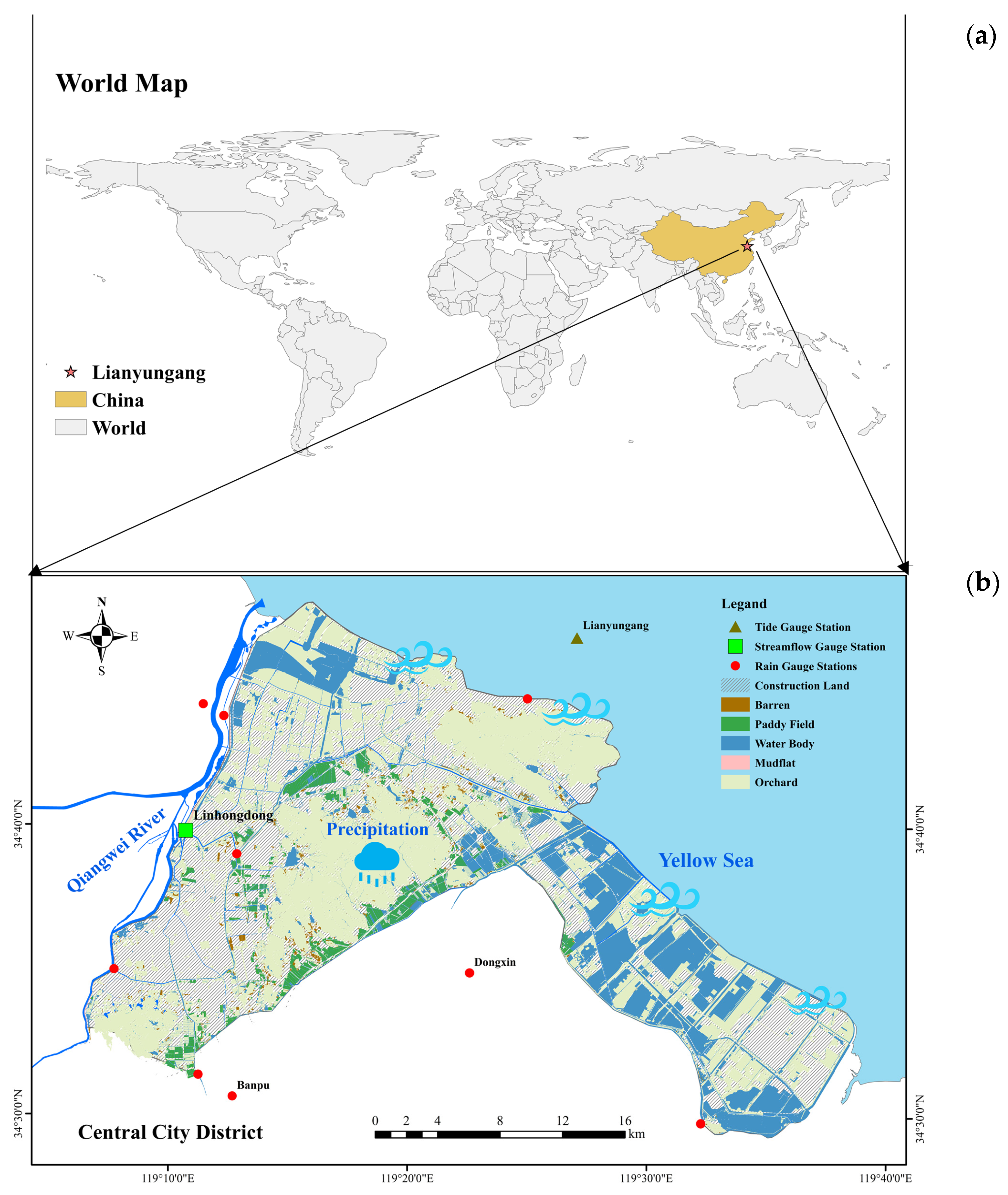
2.1.1. Study Area

The study area for this research is the Central City District of Lianyungang within Jiangsu Province in China. Lianyungang City has a total area of 5142 km², of which 1200 km² are in the central city district (Figure 1). The city’s highest point is roughly 624.4 m above sea level, whereas the eastern plain is between 2 and 3 m above. With a coastline of 176.5 km and proximity to the Yellow Sea to the east, the central city district is particularly vulnerable to compound flooding events influenced by precipitation, upstream discharge, and total water level at the coastal zones [33]. The annual water resources bulletins indicate that, from 1956 to 2020, the average annual precipitation was 904.3 mm. The highest annual rainfall occurred in 2000, with a total precipitation of 1374.3 mm. Upstream rivers, such as the Qiangwei River, have historically had maximum discharges of approximately 760 m³/s. Another hazard is high water levels; storm tide is subject to ~1.7 m above mean higher high water at Lianyungang tidal station. Furthermore, there are intense anthropogenic interventions, such as industries and inhabitants, in this complex system. The land area used for urban construction in this region increased by 32.26% between 2012 and 2022. Lianyungang City’s permanent resident population density was 2450 inhabitants per square kilometer in 2022. The data on stormwater gates, land use, and drainage canals have been gathered (

Table 1. The station is used for Statistical Analysis and Model Calibration.

Station Name	Station ID	Data Availability	Objective	Location
Lianyungang	51301300	1972 to present	Statistical Analysis Boundary Condition	119°27′00″ E, 34°46′29″ N
Xilian Island	51321950	1972 to present	Statistical Analysis Boundary Condition	119°26′10″ E, 34°46′49″ N
Linhong	51113800	1972 to present	Statistical Analysis Boundary Condition	119°12′11″ E, 34°43′50″ N
Dongxin	51127250	1972 to present	Statistical Analysis Boundary Condition	119°22′55″ E, 35°32′50″ N
Banpu	511E2503	1972 to present	Statistical Analysis Boundary Condition	119°14′35″ E, 34°27′54″ N
Linhongdong	-	1972 to present	Statistical Analysis Boundary Condition	119°09′ E, 34°37′ N
Riverside Park		2023 to 2024	Calibration	119°12′32″ E, 34°35′38″ N
Phoenix Mouth		2023 to 2024	Calibration	119°22′48″ E, 34°38′00″ N
Yudai River		2023 to 2024	Calibration	119°10′19″ E, 34°34′39″ N
Longwei River		2023 to 2024	Calibration	119°10′12″ E, 34°36′54″ N
Dapu Branch River		2023 to 2024	Calibration	119°12′41″ E, 34°39′01″ N

). As a result, Lianyungang’s Central City District makes an excellent case study for modeling and evaluating compound hazards.

2.1.2. Data Sources

The three main variables in the dataset used in this analysis are upstream river discharge (Q), total water level (Z), and precipitation (P), all of which were hourly observed data from 1972 to 2023. The total water level data were obtained from a tidal gauge station situated in Lianyungang (station id 51301300), Jiangsu, China, and were provided by the Lianyungang Branch of the Jiangsu Provincial Bureau of Hydrology and Water Resources Survey. The geographic location of this tidal gauge is 119°27′00″ E, 34°46′29″ N. The data were collected with reference to the local datum CD, and the nearest significant river is the Qiangwei River. The Qiangwei River, with a length of 59 km, ultimately discharges into the Yellow Sea, and its historical discharge at the river mouth is approximately 5910 m³/s. The central district of Lianyungang City, within low-lying areas close to the ocean and Qiangwei River, is vulnerable to coastal and river flooding. The Linhongdong Station, with geographical coordinates of 119°09′ E, 34°37′ N, was chosen to represent the Qiangwei River.

The precipitation data were collected from four national rain gauge stations and five municipal self-built rain gauge stations. The national rain gauge stations include Linhong (station id 51113800) located at 119°12′11″ E, 34°43′50″ N, Xilian Island (station id 51321950) at 119°26′10″ E, 34°46′49″ N, Banpu (station id 511E2503) at 119°14′35″ E, 34°27′54″ N, and Dongxin (station id 51127250) at 119°22′55″ E, 35°32′50″ N. The precipitation data from these stations accurately depict the precipitation patterns of Lianyungang’s central district. The distances between the precipitation, total water level, and river discharge stations are all within 50 km, ensuring the consistency and comparability of the data collection. Less than 15% of the data from the chosen stations (fluvial, coastal, and pluvial data) is missing. Several notable tropical cyclone events, including Fireworks, Muifa, and Butterfly, hit the area during this time. Typhoons are frequently followed by heavy rains, which can worsen coastal flooding by raising sea levels through the backwater effect of storm surges.

To facilitate the analysis, data processing was conducted to extract the annual maximum values of total water level, river discharge, and precipitation from the hourly monitored data. The descriptive statistics of these yearly maximum values, which include the highest, lowest, and average values recorded between 1972 and 2023, are shown in

Table 2. Statistical table of compound flood characteristics for three variables.

Item	Maximum Daily Rainfall (mm)	Highest Total Water Level (m)	Maximum River Discharge (m3/s)
Minimum	2.100	−0.047	8.970
Maximum	3.700	1.940	5910.000
Range	1.600	1.987	5901.030
First Quartile	2.430	0.188	127.500
Median	2.790	0.302	184.000
Third Quartile	3.120	0.424	240.500
Mean	2.790	0.303	1871.063
Variance	0.070	0.001	3,072,726.000
Standard Deviation	0.260	0.032	1752.341
Standard Error of the Mean	0.026	0.003	58.740
Standard Error of the Variance	0.001	0.0001	9317.000

. The data for maximum daily rainfall and highest total water level exhibit similar distribution patterns. The maximum daily rainfall has a mean of 2.790 mm and a median of 2.790 mm, while the highest total water level has a mean of 0.303 m and a median of 0.302 m. The close alignment of the mean and median values for both variables indicates symmetrical distributions, suggesting the absence of significant outliers or extreme events. The range of rainfall values is 1.600 mm with a standard deviation of 0.260 mm, and the range of water levels is 1.987 m with a standard deviation of 0.032 m, further supporting the notion of relatively uniform distributions without pronounced skewness. In contrast, the MRD data show a clearly right-skewed distribution, with a mean significantly higher than the median. This characteristic indicates the presence of extreme events that decisively influence the variability of river discharge. Specifically, the mean MRD is 1871.063 m³/s, while the median is 184.000 m³/s, indicating a significant skewness in the data. This skewness highlights the importance of using advanced probabilistic models to capture the variability and extreme events in flood risk assessment.

2.1.3. Extraction of Flood Characteristics

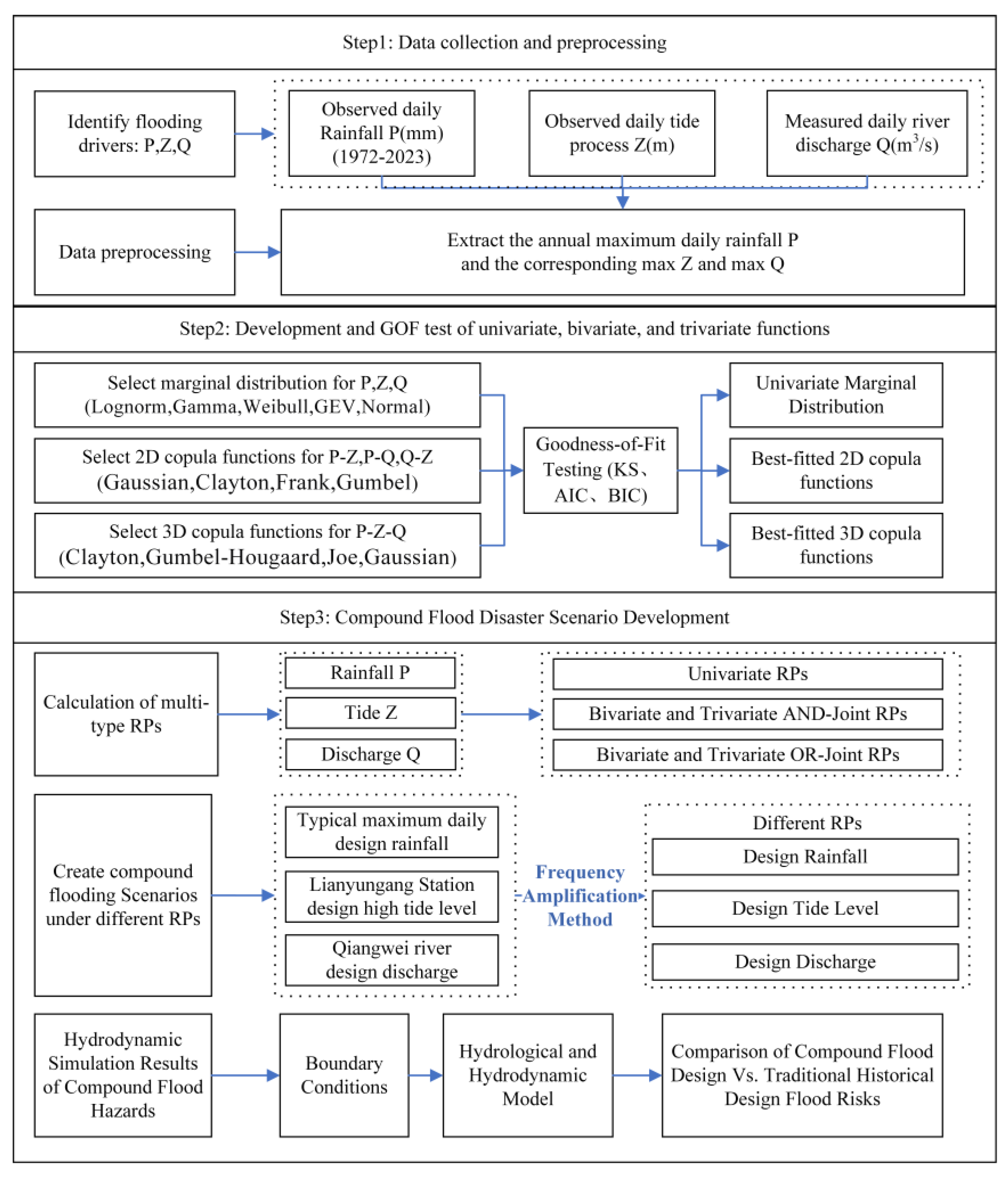
Composite flood occurrences are often identified by comparing the occurrence date of the first variable (i.e., the yearly maximum 24-h precipitation sequence) with the second and third variables (i.e., the highest water level and the maximum river discharge) [34]. This study explores the interaction between flood variables at different lag times (±1 day, ±2 days, ±3 days, ±4 days, and ±5 days). In order to identify other flood variables, the annual maximum daily precipitation was first calculated using historical observations. The correlation among these variables was then analyzed using Pearson, Kendall, and Spearman coefficients [9]. These results show that there is the strongest relationship between the maximum tide level and the annual maximum daily precipitation within a ±4-day time interval. The correlation coefficient results for the three variables are presented in

Table 3. Correlation Coefficients for the Dependence of Different Flood Characteristics (lag time = ±4 days).

Correlation Coefficient Type	Annual Maximum Daily Precipitation—Maximum Water Level (±4 days)	Annual Maximum Daily Precipitation—Maximum River Discharge (±4 days)	Maximum Total Water Level—Maximum River Discharge (±4 days)
Pearson	0.41	0.36	0.07
Kendall	0.29	0.23	−0.04
Spearman	0.42	0.36	−0.07

.

2.2. Methodology

In this study, compound flooding triggered by P, Z, and Q was analyzed. As shown in Figure 2, the first step in developing a statistical model was choosing appropriate univariate probability distributions for P, Z, and Q. For the five marginal distribution functions, both simulated and historical data were used to produce three Cumulative Distribution Functions (CDFs), Quantile-Quantile (QQ) plots, and Probability-Probability (PP) plots. To validate each fit, goodness-of-fit tests were employed, such as the Kolmogorov-Smirnov test (or K-S) [34], Akaike Information criteria (or AIC) [35], and Schwartz’s Bayesian Information criteria (or BIC) [36]. The best-fitting distribution for each variable was chosen by using maximum likelihood estimation (MLE). Then, 2D and 3D Copula functions were utilized to simulate the joint probability distributions of the specified flood variables. The final step involved flood hazard assessment and the construction of compound flood scenarios. The return periods and design values for univariate, bivariate, and trivariate flood events were determined using the Copula models and the derived probability distribution functions. The presented methodology can estimate the hazard of compound flood events under different scenarios, providing a scientific basis for flood hazard management in coastal cities.

2.2.1. Statistical Model

1.

Marginal Distribution Functions

Five commonly used univariate distribution functions for hydrological analysis are selected to fit the distributions of precipitation, total water level, and river discharge. These distribution functions include Lognormal, Gamma, Weibull, Generalized Extreme Value (GEV), and Normal distributions.

2.

Copula Functions

Commonly used 2D Copula functions in hydrological analyses include Gaussian, Clayton, Frank, and Gumbel Copulas. For 3D Archimedean Copula functions, Clayton, Gumbel-Hougaard, Joe, and Gaussian Copulas are employed. This study utilizes these 2D Copulas and 3D Archimedean Copula functions to construct the joint distribution of high-dimensional disaster-causing factors.

Gaussian Copula Function (2D Copula)

The bivariate normal distribution and density functions are given by Equations (1) and (2), where $\rho$ is the linear correlation coefficient.

$$C(u,v)={\displaystyle {\int }_{-\infty }^{{\mathsf{\Phi }}^{-1}(u)}{\displaystyle {\int }_{-\infty }^{{\mathsf{\Phi }}^{-1}(v)}\frac{1}{2\pi \sqrt{1-{\rho }^2}}\exp \left(\frac{-\left(r^2+s^2-2\rho rs\right)}{2\left(1-{\rho }^2\right)}\right)}}drds$$

(1)

$$c(u,v)={\displaystyle \frac{1}{\sqrt{1-{\rho }^2}}}\exp \left(-{\displaystyle \frac{{\mathsf{\Phi }}^{-1}{\left(u\right)}^2+{\mathsf{\Phi }}^{-1}{\left(v\right)}^2-2\rho {\mathsf{\Phi }}^{-1}\left(u\right){\mathsf{\Phi }}^{-1}\left(v\right)}{2\left(1-{\rho }^2\right)}}\right)\exp \left(-{\displaystyle \frac{{\mathsf{\Phi }}^{-1}{\left(u\right)}^2•{\mathsf{\Phi }}^{-1}{\left(v\right)}^2}{2}}\right)$$

(2)

Clayton Copula Function (2D Copula)

The bivariate distribution and density functions are given by Equations (3) and (4), with $\theta$ being the parameter of the generator, $\phi (t)={\displaystyle \frac{1}{\theta }}\left(t^{-\theta }-1\right)$, and related to the Kendall rank correlation coefficient τ by $\tau =\theta /(\theta +2)$.

$$C(u,v)={(u^{-\theta }+v^{-\theta }-1)}^{-1/\theta }$$

(3)

$$c(u,v)=\left(1+\theta \right){\left(uv\right)}^{-\theta -1}{(u^{-\theta }+v^{-\theta }-1)}^{-2-1/\theta }$$

(4)

Frank Copula Function

The bivariate distribution and density functions are given by Equations (5) and (6), with $\theta$ being the parameter of the generator, $\phi (t)=-\ln \left({\displaystyle \frac{e^{-\theta t}-1}{e^{-\theta }-1}}\right)$, and related to the Kendall correlation coefficient τ by $\tau =1+{\displaystyle \frac{4}{\theta }}\left(D_1\left(\theta \right)-1\right)$, $D_1\left(\theta \right)={\displaystyle \frac{1}{\theta }}{\displaystyle {\int }_0^{\theta }\frac{t}{e^t-1}dt}$.

$$C\left(u,v\right)=-{\displaystyle \frac{1}{\theta }}ln\left[1+{\displaystyle \frac{\left(e^{-\theta u}-1\right)\left(e^{-\theta v}-1\right)}{e^{-\theta }-1}}\right]$$

(5)

$$c\left(u,v\right)={\displaystyle \frac{-\theta \left(e^{-\theta }-1\right)e^{-\theta \left(u+v\right)}}{{\left[\left(e^{-\theta }-1\right)+\left(e^{-\theta u}-1\right)\left(e^{-\theta v}-1\right)\right]}^2}}$$

(6)

Gumbel Copula Function

The bivariate distribution and density functions are given by Equations (7) and (8), with $\theta$ being the parameter of the generator, $\phi (t)={(-\ln t)}^{\theta }$, and related to the Kendall rank correlation coefficient τ.

$$C(u,v)=\exp \left\{-{\left[{\left(-\ln u\right)}^{\theta }+{\left(-\ln v\right)}^{\theta }\right]}^{1/\theta }\right\}$$

(7)

$$c(u,v)={\displaystyle \frac{C(u,v){\left(\ln u\cdot \ln v\right)}^{\theta -1}}{uv{\left[{\left(-\ln u\right)}^{\theta }+{\left(-\ln v\right)}^{\theta }\right]}^{2-{\theta }^{-1}}}}\left\{{\left[{\left(-\ln u\right)}^{\theta }+{\left(-\ln v\right)}^{\theta }\right]}^{{\theta }^{-1}}+\theta -1\right\}$$

(8)

For 3D Archimedean Copula joint distribution functions, the following are used:

Clayton Copula Function (3D Copula)

The trivariate distribution and density functions are given by Equation (9):

$$C(u,v,w)={\left(u^{{\displaystyle \frac{-1}{\theta }}}+v^{{\displaystyle \frac{-1}{\theta }}}+{\mathrm{w}}^{{\displaystyle \frac{-1}{\theta }}}-2\right)}^{-\theta }$$

(9)

Gumbel-Hougaard Copula Function

The trivariate distribution and density functions are given by Equation (10), with $\theta$ as the parameter of the generator, $\phi (t)={(-\ln t)}^{\theta }$:

$$C(u,v,w)=e^{\left(-{\left[{\left(-\ln u\right)}^{\theta }+{\left(-\ln v\right)}^{\theta }+{\left(-\ln w\right)}^{\theta }\right]}^{1/\theta }\right)}$$

(10)

Gaussian Copula Function (3D Copula)

The trivariate distribution and density functions are given by Equation (11):

$$C(u,v,w)=1-{\left[{\left(1-u\right)}^{\theta }+{\left(1-v\right)}^{\theta }+{\left(1-w\right)}^{\theta }-{(1-u)}^{\theta }{\left(1-v\right)}^{\theta }{\left(1-w\right)}^{\theta }\right]}^{1/\theta }$$

(11)

Joe Copula Function

The trivariate distribution and density functions are given by Equation (12):

$$C(u,v,w)={\mathsf{\Phi }}_R\left({\varphi }^{-1}\left(u\right),{\varphi }^{-1}\left(v\right),{\varphi }^{-1}\left(w\right)\right)$$

(12)

where $\theta$ is the parameter of the generator, $\phi (t)={(-\ln t)}^{\theta }$. ${\mathsf{\Phi }}_R$ is the joint cumulative distribution function of a standard trivariate normal distribution with correlation matrix R, and ${\varphi }^{-1}$ is the inverse cumulative distribution function of the standard univariate normal distribution.

3.

Goodness-of-Fit Testing

Given the limitations in the time span of sample sequences, the sample size is often restricted. In such cases, fitting tests for joint distribution functions are essential to validate whether the chosen joint distribution functions effectively represent the actual characteristics of joint probability events. Goodness-of-fit tests help identify the theoretically optimal model from multiple candidate joint distribution functions for calculating joint probabilities. This study utilizes the Kolmogorov-Smirnov (K-S) test, Akaike Information Criterion (AIC), Bayesian Information Criterion (BIC), and Cramér-von Mises (CvM) test statistics to evaluate the goodness-of-fit of Copula functions.

2.2.2. Joint Probability Distribution and Return Periods

In hydrological analysis, the return period is a commonly used measure to quantify the probability of the occurrence of rare events. This section provides a detailed introduction to the univariate, bivariate, and multivariate return periods.

Univariate Return Period

The return period is a concept that refers to the average number of years between occurrences of a disastrous event $X\ge x$. Given a disastrous factor x, its univariate return period can be estimated using the cumulative distribution function (CDF) derived from the best-fitting probability distribution:

$$T_X={\displaystyle \frac{1}{P(X\ge x)}}={\displaystyle \frac{1}{1-F_X(x)}}={\displaystyle \frac{1}{1-CDF(x)}}$$

(13)

where F(x) is the univariate cumulative distribution function value obtained from the best-fitting probability distribution.

Bivariate Return Period

For flood events in coastal cities, if one of two disastrous factors exceeds a certain threshold (e.g., $X\ge xORY\ge y$), it can lead to a flood event. The return period when either variable exceeds a threshold is called the joint return period and can be calculated as:

$$T_{X,Y}^{OR}={\displaystyle \frac{1}{P(X\ge xORY\ge y)}}={\displaystyle \frac{1}{1-H(x,y)}}={\displaystyle \frac{1}{1-C(F_X(x),G_Y(y))}}$$

(14)

where $F_X(x)$ and $G_Y(y)$ are the univariate marginal cumulative distribution functions obtained from the best-fitting probability functions, and $H(x,y)$ is the bivariate joint cumulative distribution function based on the Copula.

If both variables exceed their respective thresholds (e.g., $X\ge xANDY\ge y$), coastal cities are more prone to severe flood events. The return period for both variables exceeding their thresholds is called the copula-based simultaneous return period and can be calculated as:

$$\begin{array}{ll}{T}_{X,Y}^{AND}& ={\displaystyle \frac{1}{P(X\ge xANDY\ge y)}}={\displaystyle \frac{1}{1-F_X(\mathrm{x})-F_Y(y)+H(x,y)}}\hfill \\ & ={\displaystyle \frac{1}{1-F_X(\mathrm{x})-F_Y(y)+C(F_X(x),F_Y(y))}}\hfill \end{array}$$

(15)

Multivariate Return Period

For the trivariate joint distribution scenario (simulated through 3D Copula), the joint return period (e.g., $X\ge xORY\ge yORZ\ge z$) and the simultaneous return period (e.g., $X\ge x\&Y\ge y\&Z\ge z$) can be calculated using the following formulas:

$$\begin{array}{ll}{T}_{X,Y,Z}^{OR}& ={\displaystyle \frac{1}{P(X\ge x\cup Y\ge y\cup Z\ge z)}}={\displaystyle \frac{1}{1-H(x,y,z)}}\hfill \\ & ={\displaystyle \frac{1}{1-C(F_X(x),F_Y(y),F_Z(z))}}\hfill \end{array}$$

(16)

$$\begin{array}{ll}{T}_{X,Y,Z}^{AND}& ={\displaystyle \frac{1}{P(X\ge x\cap Y\ge y\cap Z\ge z)}}\hfill \\ & ={\displaystyle \frac{1}{1-F_X(x)-F_Y(y)-F_Z(z)+H(x,y)+H(y,z)+H(z,x)-H(x,y,z)}}\hfill \end{array}$$

(17)

2.2.3. Hydrodynamic Model Setup

Hydrological Model

This model is developed using a distributed combined hydrological modeling approach [37,38], dividing the urban area into two parts: plain and mountainous regions. The plain region is further categorized into six classes—urban land, dry land, paddy fields, water surfaces, green spaces, and tidal flats. For the plain region, the Soil Conservation Service (SCS) model, which is suitable for dry land, and the constant coefficient model, applicable to impervious urban areas, were combined. The Curve Number (CN) was set between 60 and 80, and the initial abstraction (Ia) was set at 0.2 based on the interpretation of soil types and land use types in the central city district of Lianyungang City. The study area also includes the mountainous regions of Yuntaishan and Jinpingshan, whose hydrological characteristics significantly differ from those of the urban areas. Therefore, the Probability Distributed Model (PDM) was employed to simulate the runoff generation and routing in these regions. The standard runoff percentage was set at 0.29. The nonlinear reflow characteristics of the runoff are described using the Izzard method, with a p coefficient of 0.333.

1D River Network Hydrodynamic Model

The one-dimensional river network model employs the Saint-Venant equations to describe water balance and flow dynamics within water channels. The governing equations are as follows:

$${\displaystyle \frac{\partial Q}{\partial x}}+B{\displaystyle \frac{\partial Z}{\partial t}}=0$$

(18)

$${\displaystyle \frac{\partial Q}{\partial t}}+{\displaystyle \frac{\partial }{\partial x}}(Qu)+gA{\displaystyle \frac{\partial h}{\partial x}}-gA{s}_0+gA{s}_f=0$$

(19)

where Q represents the flow rate, m³/s; A represents the cross-sectional area of flow, m²; h represents the water depth, m; s₀ represents the bed slope; s_f represents the friction slope; and u represents the average cross-sectional velocity, m/s. The governing equations are solved using the finite difference method. The Preissmann four-point implicit scheme, which is known for its strong convergence and stability, is employed for discretization. The 1D river network model for the central urban area of Lianyungang City comprises 535 channels with a total length of 606 km. The model also describes 1211 channel cross-sections and the operation rules of 127 water gates and pump stations. The spacing of the measured river cross-sections was approximately 100 to 500 m. Based on empirical values, the roughness coefficient of the river channel was set to a range of 0.02~0.04. The maximum computational step length for the model was 100 m. To ensure the stability and accuracy of the model calculations, the time step was determined to be 60 s through model calibration and debugging.

1D Pipe Network Model

The control equations for the pipe network model are the Saint-Venant equations, which consist of the continuity equation (mass conservation) and the momentum equation. The control equations are as follows:

$${\displaystyle \frac{\partial C}{\partial t}}+{\displaystyle \frac{\partial Q}{\partial x}}=0$$

(20)

$${\displaystyle \frac{\partial Q}{\partial t}}+{\displaystyle \frac{\partial }{\partial x}}\left({\displaystyle \frac{Q^2}{C}}\right)+gC\left(\cos \theta {\displaystyle \frac{\partial h}{\partial x}}-i+{\displaystyle \frac{Q\left|Q\right|}{K^2}}\right)=0$$

(21)

where Q represents the flow rate, m³/s; C represents the cross-sectional area of the pipe in m²; g represents the acceleration due to gravity, m/s²; θ represents the angle between the pipe bottom and the horizontal plane, degrees; h represents the water depth in meters; i represents the slope of the pipe; K represents the coefficient based on the Colebrook-White or Manning’s formula, m³/s. During the modeling process, the 1D pipe network model for the central city district of Lianyungang City was preprocessed using ArcGIS 10.6 software. This preprocessing involved the manipulation of pipe and 1D manhole data to ensure the stability and accuracy of model calculations. Specifically, short pipes and isolated manholes, which could potentially affect the stability of model computations, were removed. Additionally, the topological structure of the pipe network system was established to facilitate the seamless integration and functioning of the network. After these preprocessing steps, the resulting drainage pipe network comprised 36,702 segments with a total length of 1302.10 km and 37,838 manholes (Figure 3).

1D and 2D Coupled Flood Propagation Model

$${\displaystyle \frac{\partial h}{\partial t}}+{\displaystyle \frac{\partial (hu)}{\partial x}}+{\displaystyle \frac{\partial (hv)}{\partial y}}={\displaystyle {\sum }_{i=1}^n{q}_i}$$

(22)

$$\begin{array}{l}{\displaystyle \frac{\partial (hu)}{\partial t}}+{\displaystyle \frac{\partial }{\partial x}}\left(h{u}^2+{\displaystyle \frac{g{h}^2}{2}}\right)+{\displaystyle \frac{\partial (huv)}{\partial y}}-{\displaystyle \frac{\partial }{\partial x}}(\epsilon h{\displaystyle \frac{\partial u}{\partial x}})-{\displaystyle \frac{\partial }{\partial y}}(\epsilon h{\displaystyle \frac{\partial u}{\partial y}})\\ =gh(S_{0,x}-S_{f,x})+{\displaystyle {\sum }_{i=1}^n{q}_i{u}_i}\end{array}$$

(23)

$$\begin{array}{l}{\displaystyle \frac{\partial (hv)}{\partial t}}+{\displaystyle \frac{\partial }{\partial y}}\left(h{v}^2+{\displaystyle \frac{g{h}^2}{2}}\right)+{\displaystyle \frac{\partial (huv)}{\partial x}}-{\displaystyle \frac{\partial }{\partial x}}(\epsilon h{\displaystyle \frac{\partial v}{\partial x}})-{\displaystyle \frac{\partial }{\partial y}}(\epsilon h{\displaystyle \frac{\partial v}{\partial y}})\\ =gh(S_{0,y}-S_{f,y})+{\displaystyle {\sum }_{i=1}^n{q}_i{v}_i}\end{array}$$

(24)

where h represents the water depth, m; u and v are the velocity components in the x and y directions, respectively, m/s; q_i is the source flow generated by rainfall on the grid cell, m/s; u_i and v_i are the velocities produced by rainfall on the grid cell, m/s; g is the acceleration due to gravity, m²/s; ε is the eddy viscosity coefficient, m²/s; S_0,x and S_0,y are the bed slopes in the x and y directions, respectively; S_f,x and S_f,y represent the bed friction in the x and y directions, respectively; n is the number of source terms. In this study, rainfall was directly applied to the 2D computational mesh. The overland flow routing was simulated using a 2D modeling approach, which takes into account the elevation differences between mesh cells. When the floodwater depth exceeds the elevation of the riverbanks, an exchange of flow occurs between the river channel and the inundated areas. In this study, this model utilized high-resolution digital elevation data to discretize the study area into 89,544 unstructured triangular meshes. The inflow process was employed as the upper boundary condition, while the total water level was used as the lower boundary condition. The foundational files used for combined model construction are depicted in Figure 4.

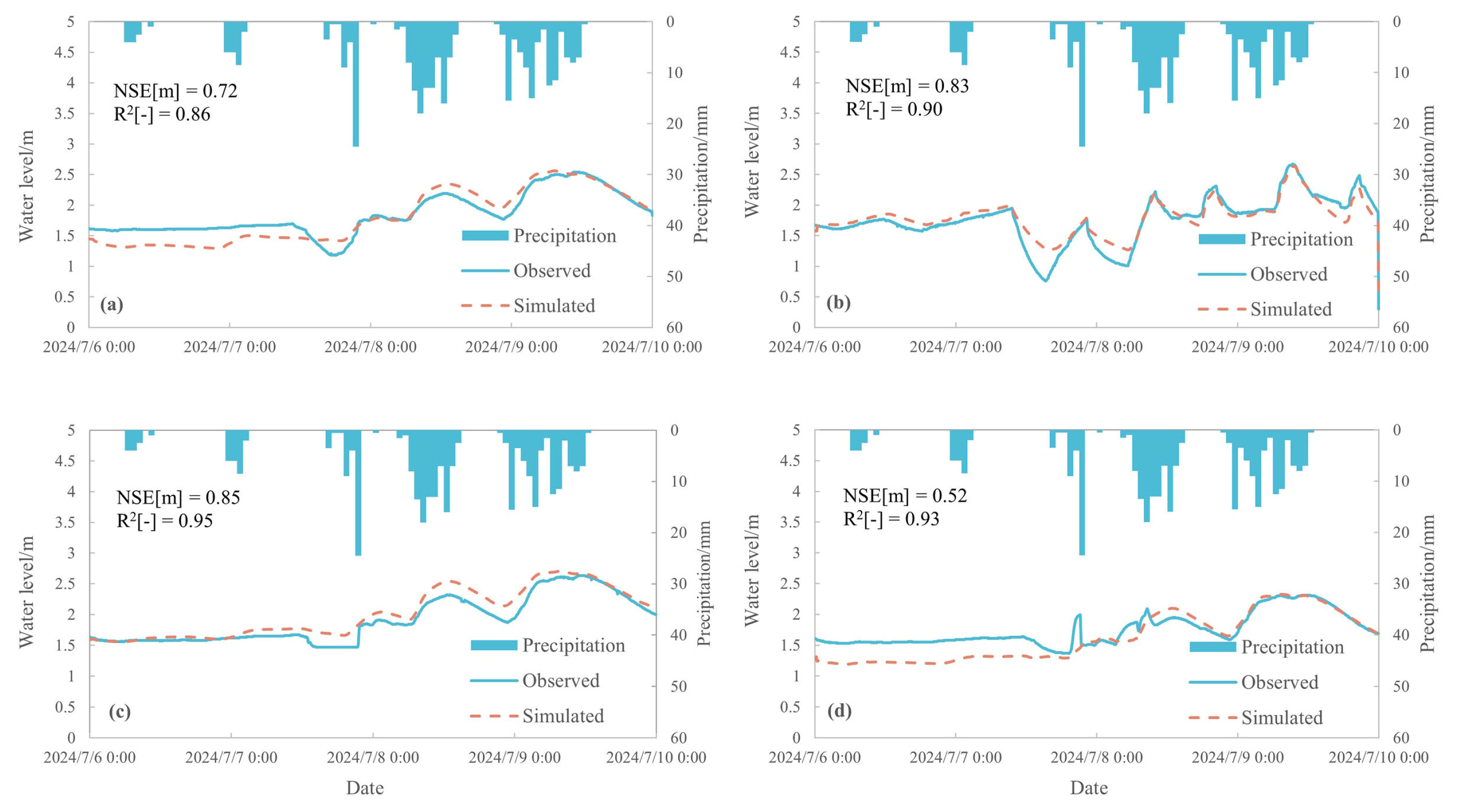
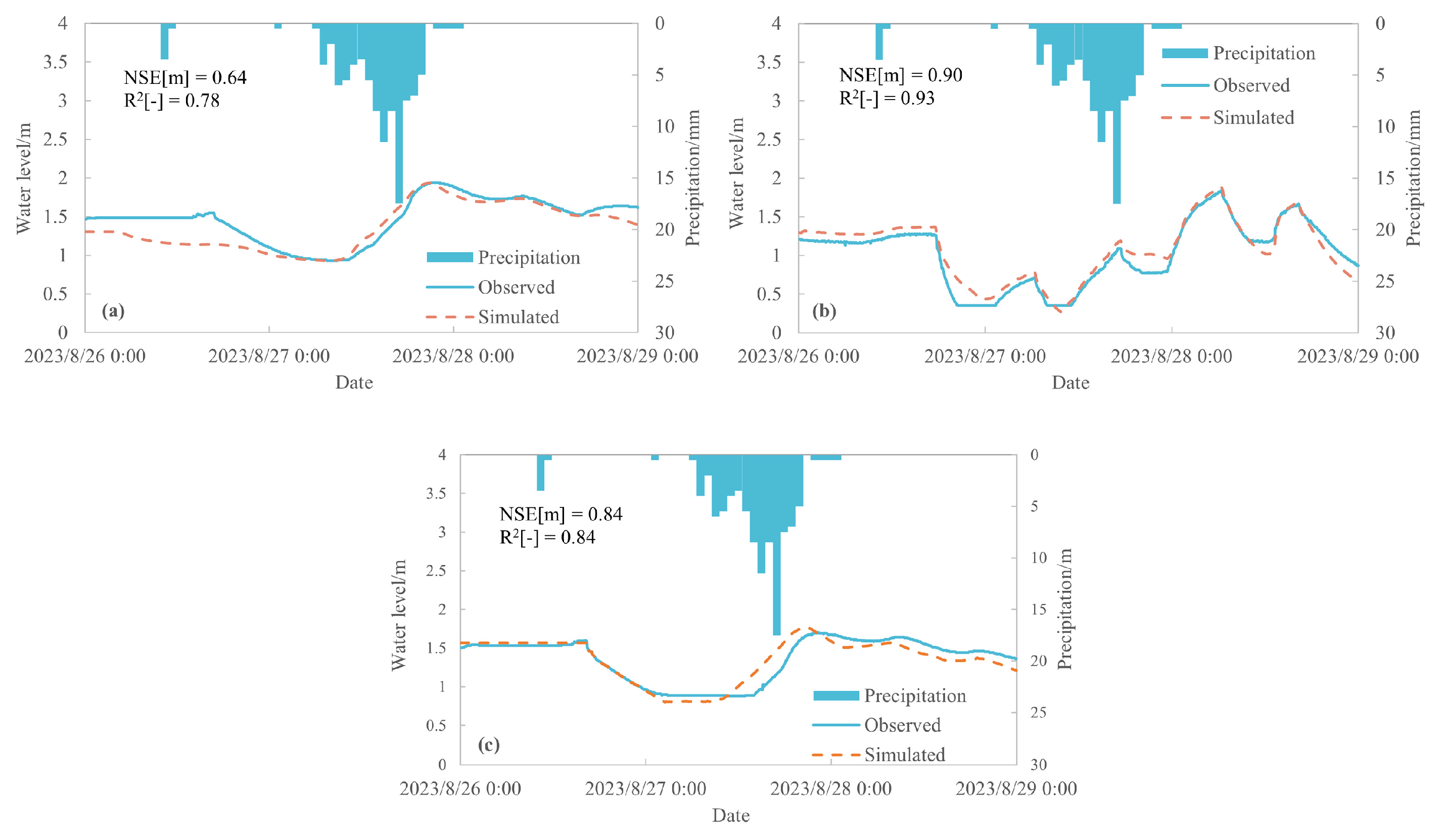
2.2.4. Model Calibration

The performance of the model was evaluated using the Nash-Sutcliffe Efficiency (NSE) and the Coefficient of Determination (R²) between model observations and simulations for a 3 to 4-day simulation period in the past 5 years. In general, NSEs above 0.70 m (water level) are desirable for urban flood modeling in China [39]; however, small NSEs (0.64 m) have been reported in model simulations of a real flood event in Omihachiman City, Japan [40]. The equations are as follows:

$$\mathrm{NSE}=1-\left[{\displaystyle \frac{{\displaystyle {\sum }_{i=1}^n{\left(Y_i^{obs}-Y_i^{sim}\right)}^2}}{{\displaystyle {\sum }_{i=1}^n{\left(Y_i^{obs}-Y^{mean}\right)}^2}}}\right]$$

(25)

where Y_i^obs is the i-th observed data series, Y_i^sim is the i-th simulated data, Y_i^mean is the mean of the observed data series, and n is the total number of observed data.

$$R^2={\displaystyle \frac{{\left({\displaystyle \sum \left(Y^{obs}-\overline{Y^{obs}}\right)\left(Y^{sim}-\overline{Y^{sim}}\right)}\right)}^2}{{\displaystyle \sum {\left(Y^{obs}-\overline{Y^{obs}}\right)}^2{\displaystyle \sum {\left(Y^{sim}-\overline{Y^{sim}}\right)}^2}}}}$$

(26)

where Y^obs is the observed data series; $\overline{Y^{obs}}$ is the mean of the observed data series; Y^sim is the simulated data series; $\overline{Y^{sim}}$ is the mean of the observed data series, and n is the mean of the simulated data series.

Model calibration consists of simulating an extreme flood inundation event characterized by extreme coastal water levels and precipitation (recent records) as reported by Lianyungang Municipal Administration Bureau. For calibration purposes, the focus is on the rainfall event hitting the Central City District from 6–9 July 2024, during which the monitored daily rainfall exceeded 317 mm. The heavy flood from 26–28 August 2023 broke the record for the highest single-day rainfall in the Central City District since meteorological records began. Extensive flooding occurred throughout the city, with average floodwater heights ranging from 50 to 70 cm. The heavy rain also triggered a flash flood in Yuntai Mountain, trapping tourists in the rapid currents. The maximum total water level measured at Lianyungang tidal station reached 4.56 m.

The model calibration results at four sites on 6–9 July 2024 were displayed in Figure 5, while the model calibration results at five stations on 26–29 August 2023 were displayed in Figure 6. Following model parameter calibration, the following final roughness coefficients were found for the various kinds of river channels in this area: The roughness coefficient was chosen at 0.019 to 0.020 for the main channels, 0.025 for the regional channels, 0.03 for the tiny internal channels, and 0.035 for the channels in the hilly areas. For the rainfall event in 2024, the average NSE and R² were 0.73 and 0.91, respectively. The average NSE and R² for the rainfall event in 2023 were 0.75 and 0.83, respectively.

2.2.5. Integration of Statistical and Hydrodynamic Model

Although statistical models have been widely employed, their integration with hydrodynamic models is not very common. Despite being widely used to estimate coastal flood hazards, simple bathtub models frequently underestimate the consequences of flooding [41] because they are unable to account for river-tide interactions and variable nonlinear flood dynamics [42,43,44], as well as to vary flood stages with increasing distance from the coast.

By taking into account the flood impacts under particular statistical return period conditions, this work seeks to bridge the gap between statistical and hydrodynamic models. A high-resolution urban flood model is developed by using the joint probability boundary conditions obtained from statistical analysis as inputs to the hydrodynamic model. Model parameters are calibrated, and multiple dynamic simulations are conducted for the entire computation period, taking into account the actual conditions of drainage networks and associated infrastructure. This method makes scenario analysis easier by clearly illustrating the development and catastrophe process of compound flood inundation in urban areas. This article also answers the following questions: what is the extent of flood impact for a given return period, like 200 years? How does the flood hazard distribution for a coastal city differ under compound flood conditions compared to a single flood factor?

2.2.6. Steps of Amplification Flood Hazard Assessment Caused by Precipitation, River Discharge and Total Water Level

This study investigates the differences in inundation areas across various hazard levels (extreme and high) under compound flood events and univariate flood events in urban areas, as well as the factors influencing these differences. To achieve this, a linear regression analysis method was employed to establish a relationship model between the ratios of inundation areas and the ratios of precipitation, river discharge, and water level, thereby quantifying the contributions of each factor to the changes in inundation areas.

Step 1. Data Collection and Processing

Taking the extreme hazard level as an example, data from flood events with different return periods (5, 10, 25, 50, 100, and 200 years) were collected. These data included six sets of Compound Flood (CF)scenarios (denoted as Z1, Q1, P1) and single-frequency flood scenarios (denoted as Z2, Q2, P2), as well as the corresponding hydrodynamic calculation results, namely the inundation areas A1 and A2 for different risk levels. Here, P1 and P2 represent the precipitation under compound flood and single-frequency flood events, respectively; Q1 and Q2 represent the river discharge rates; Z1 and Z2 represent the water levels; and A1 and A2 represent the corresponding inundation areas. The data collection and processing for high levels were conducted in the same manner.

Step 2. Model Establishment

To quantify the differences in inundation areas across various risk levels under compound flood events and single-frequency flood events and to identify the influencing factors, the following linear relationship model was established:

$${\displaystyle \frac{A_2}{A_1}}=b_1\times {\displaystyle \frac{P_2}{P_1}}+b_2\times {\displaystyle \frac{Q_2}{Q_1}}+b_3\times {\displaystyle \frac{Z_2}{Z_1}}+m$$

(27)

where ${\displaystyle \frac{A_2}{A_1}}$ represents the amplification ratio of inundation areas for specific hazard; ${\displaystyle \frac{P_2}{P_1}}$, ${\displaystyle \frac{Q_2}{Q_1}}$, and ${\displaystyle \frac{Z_2}{Z_1}}$ represent the amplification ratios of maximum precipitation, discharge, and total water level, respectively; b₁, b₂, and b₃ are the coefficients to be estimated, which quantify the contributions of each factor to the changes in inundation areas; and m is a constant term, representing the impact of other factors on the changes in inundation areas, including urban drainage systems, land use and other human-induced factors.

Step 3. Parameter Estimation and Model Validation

Nonlinear Least Squares were used to estimate the parameters of the model. The relevant functions in MATLAB R2023b were employed to fit the model, yielding the estimated values of b₁, b₂, b₃, and m. Additionally, statistical indicators of the model, including the R² and SEE, were calculated to assess the model’s fit and significance. The model fitting and parameter estimation were conducted separately for extremely high and high hazard levels to comprehensively evaluate the impact of each factor on the changes in inundation areas.

3. Results

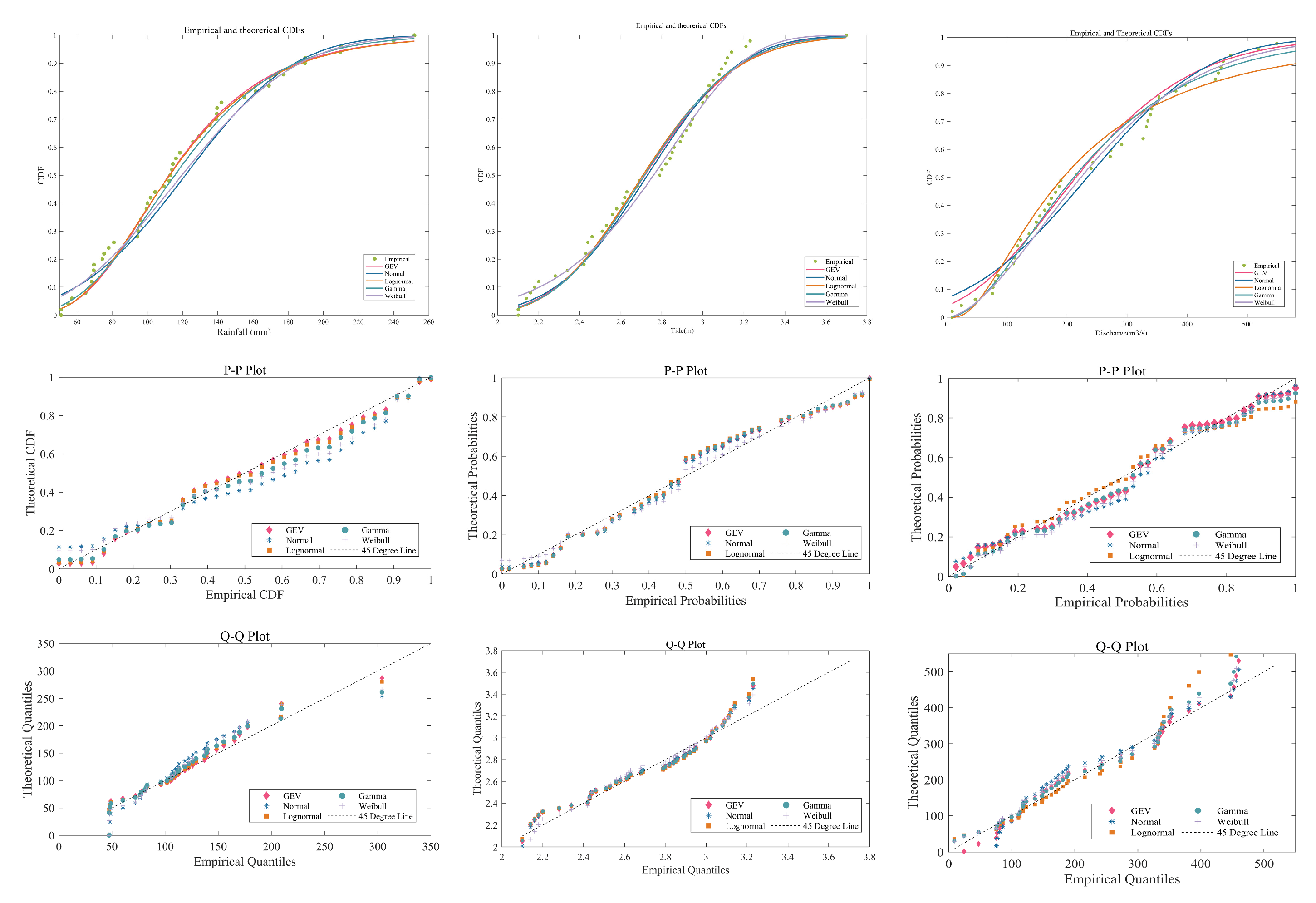
3.1. Performance of Marginal Distributions

According to the fitting findings displayed in

Table 4. Goodness-of-Fit Test for Marginal Distribution Functions, (a) Maximum Daily Precipitation, (b) Maximum Total Water Level, (c) Maximum River Discharge.

(a) Maximum Daily Precipitation
Marginal Distribution	K-S	AIC	BIC
Lognormal	0.0673	524.8844	528.7084
Gamma	0.0661	525.6700	529.4940
Weibull	0.0917	530.0721	533.8961
GEV	0.0713	527.4774	533.2135
Normal	0.1051	533.1909	537.0149
(b) Maximum Total Water Level
Marginal Distribution	K-S	AIC	BIC
Lognormal	0.110	40.8555	44.6795
Gamma	0.1038	40.4649	44.2890
Weibull	0.0701	43.7835	47.6076
GEV	0.0993	42.4552	48.1913
Normal	0.0873	40.3883	44.2123
(c) Maximum River Discharge
Marginal Distribution	K-S	AIC	BIC
Lognormal	0.1178	614.1941	617.8944
Gamma	0.1223	603.7056	607.4059
Weibull	0.1134	601.3576	605.0579
GEV	0.1133	649.8128	655.5489
Normal	0.1295	651.0001	654.8242

, the Gamma distribution best describes the statistical characteristics of precipitation data, as shown by its strong performance in terms of AIC, BIC, and K-S test statistics. With better AIC and BIC scores and a reduced K-S statistic, the Weibull distribution is the best model to fit the tidal data. The GEV distribution stands out with the lowest K-S test score for discharge data, indicating a more accurate fit to the distribution. For various marginal distributions of precipitation, total water level, and river discharge, Figure 7 displays the quantile-quantile (Q-Q), cumulative distribution (CDF), and probability-probability (P-P) plots, respectively.

3.2. Copula Function in Bivariate Modeling and Estimation of Dependency Parameters

Multivariate joint modeling is an essential tool for analyzing and quantifying the complex dependencies among multiple random variables. The first stage of trivariate joint modeling in this study focused on simulating bivariate dependencies. Multiple 2D Copula functions were used to estimate the joint cumulative distribution functions (JCDFs). Bivariate joint probability distribution models for P-Z, P-Q, and Z-Q were developed using Gaussian, Gumbel, Clayton, and Frank Copula functions based on the optimal marginal distribution functions for P, Z, and Q that were determined in Section 3.1.

Table 5. Maximum Likelihood Estimation (MLE) Method for Bivariate Copula Parameters and Goodness-of-Fit, (a) P-Z, (b) Z-Q, (c) P-Q.

(a) P-Z
Copula	AIC	BIC	$\mathit{\theta }$	Sn (N = 1000)
Gaussian	−7.5330	−4.9278	0.4311	7.3130
Clayton	−8.2468	−5.6416	0.7999	4.1063
Frank	−6.6947	−4.0896	2.5481	4.8262
Gumbel	−1.7312	0.8740	0.1959	5.9759
(b) Z-Q
Marginal Distribution	K-S		AIC	BIC
Gaussian	1.9989		4.6041	0.0048
Clayton	2.0000		4.6052	1.8649 × 10−8
Frank	4.6052		4.6052	3.0381 × 10−8
Gumbel	4.6052		4.6052	1.0000
(c) P-Q
Marginal Distribution	K-S		AIC	BIC
Gaussian	−4.3445		−1.7393	0.3427
Clayton	−1.6085		0.9967	0.4368
Frank	−4.7319		−2.1268	2.0608
Gumbel	−3.4514		−0.8462	1.2389

shows each distribution’s AIC, BIC, and K-S test results.

With the lowest AIC and BIC values and the minimum CvM statistic, which indicates the best fit to the data, the Clayton Copula was found to be the best choice for the combined distribution of P and Z. The Clayton and Gumbel copulas exhibited the best fit according to the CvM statistics, whereas the Gaussian copula was preferred in the instances of Z and Q since it had the lowest AIC. With the lowest AIC and BIC values, the Frank Copula model was clearly the best choice for simulating the joint distribution of P and Q.

3.3. Optimal Trivariate Copula Joint Modelling

Several 3D symmetric Archimedean and elliptical Copula families were used in this study. The Gumbel-Hougaard Copula performed quite well when modeling the joint distribution of P, Z, and Q as shown in

Table 6. Parameters for Symmetric 3-D Archimedean and Elliptical Copulas.

Copula Category	Copula Function	θ	AIC	BIC	N = 1000
					Sn	p-Value
Archimedean	Clayton	12.627	−25,529.233	−25,527.321	3.362	0.0
	Gumbel-Hougaard	1.173	368.126	370.038	0.001	0.425
	Joe	1.500	2,000,002	2,000,004	0.265	0.023
Elliptical	Gaussian	0.337, 0.432, 0.002	410.637	416.373	0.001	0.407

. Its benefits are as follows: (1) GH and Gaussian Copulas both showed excellent fit, with the minimum CvM and high p-values, indicating a more accurate capture of the joint distribution characteristics compared to other models (2) From an information criterion perspective, the GH Copula has the lowest AIC and BIC values. These criteria penalize model complexity to prevent overfitting, and the low values for GH Copula suggest optimal fit while maintaining model simplicity. In contrast, other Copula models, such as the Clayton Copula, despite having very low AIC and BIC values, exhibit larger CvM with p-values of zero, indicating a poor fit for the data in this study. Similarly, the Joe Copula, with very high AIC and BIC values and large CvM, was found to be less suitable for the current data analysis due to its lower p-values.

3.4. Return Periods of Univariate and Trivariate Flood Characteristics

The RPs for individual flood drivers and joint return periods for bivariate distributions are shown in

Table 7. Univariate and Bivariate Joint Return Periods (P-Z).

RPs (Years)	Annual Max Precipitation (mm)	Annual Max Total Water Level (m)	${\mathit{T}}_{\mathit{P}\mathit{Z}}^{\mathit{O}\mathit{R}}$ (Years)	${\mathit{T}}_{\mathit{P}\mathit{Z}}^{\mathit{A}\mathit{N}\mathit{D}}$ (Years)
5	158.32	3.05	2.96	16.09
10	184.28	3.19	5.46	60.05
25	207.68	3.29	10.46	231.65
50	236.18	3.39	25.42	1407.70
100	256.48	3.46	50.43	5595.00
200	275.98	3.52	100.72	22,432.00
500	300.83	3.59	249.86	138,470.00
1000	319.05	3.63	500.65	556,470.00

. Notably, OR-Joint RP is smaller than the univariate return period, which is less than the AND-Joint RP return period, assuming equivalent univariate return periods. For instance, for a maximum daily P of 256.48 mm and a highest Z value of 3.46 m within a ±4-day interval, the OR-Joint and AND-Joint return periods are 50.43 years and 5595 years, respectively. This implies that under OR conditions rather than AND conditions, bivariate flood characteristics co-occur more frequently.

Expanding to trivariate distributions, the return periods for three flood drivers were calculated. Results are presented in

Table 8. Trivariate Joint Return Periods (Precipitation-Tide Level-Discharge).

RPs (Years)	Annual Max P (mm)	Annual Max Z (m)	Annual Max Q (m3/s)	GH ${\mathit{T}}_{\mathit{P}\mathit{Z}\mathit{Q}}^{\mathit{O}\mathit{R}}$ (Years)	$\mathbf{GH} {\mathit{T}}_{\mathit{P}\mathit{Z}\mathit{Q}}^{\mathit{A}\mathit{N}\mathit{D}}$ (Years)	$\mathbf{Gaussian} {\mathit{T}}_{\mathit{P}\mathit{Z}\mathit{Q}}^{\mathit{O}\mathit{R}}$ (Years)	$\mathbf{Gaussian} {\mathit{T}}_{\mathit{P}\mathit{Z}\mathit{Q}}^{\mathit{A}\mathit{N}\mathit{D}}$ (Years)
5	158.32	3.05	354.60	2.30	25.54	2.30	22.64
10	184.28	3.19	438.80	4.24	62.70	4.11	73.04
25	207.68	3.29	513.87	8.16	137.56	7.67	233.40
50	236.18	3.39	603.39	19.88	361.10	18.12	1103.30
100	256.48	3.46	665.24	39.48	734.16	35.34	3730.17
200	275.98	3.52	722.74	78.82	1482.91	69.60	13,422.84
500	300.83	3.59	792.76	195.93	3711.86	170.85	85,061.96
1000	319.05	3.63	841.60	392.27	7448.61	339.78	49,1650.97

. These indicate that AND-Joint RP exceeds the OR-Joint RP when considering three flood characteristics, suggesting a higher frequency of simultaneous occurrence under OR- conditions compared to AND conditions.

Univariate and bivariate models overlook dependencies among multiple disasters in flood hazard analysis. The trivariate joint distribution method using the Archimedean GH Copula provides a more conservative estimate of joint return periods, which is deemed more appropriate for safety considerations. Therefore, it is recommended that future research adopt the GH Copula joint return periods for P, Z, and Q identified in this study as benchmarks for engineering design.

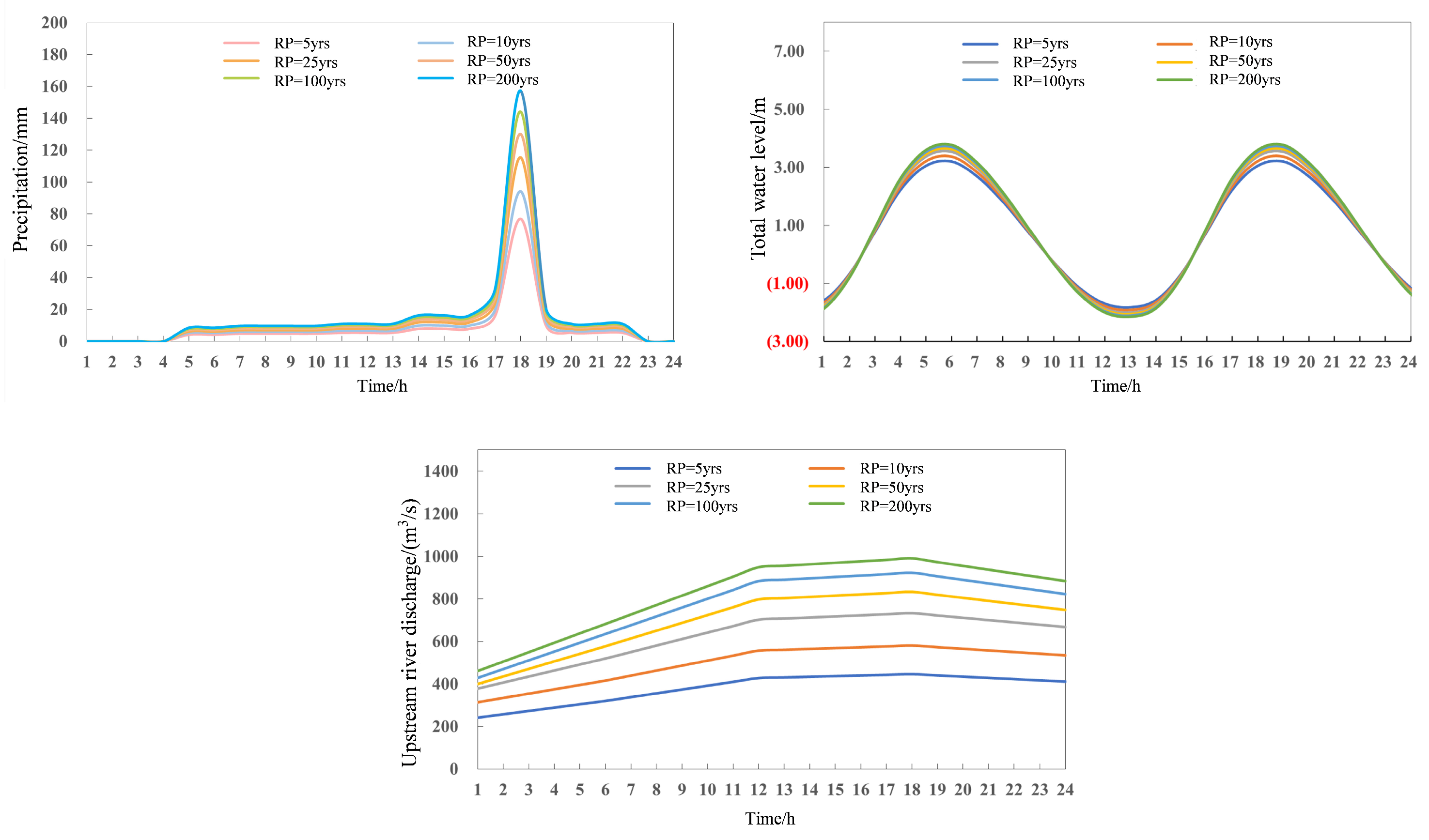
3.5. Compound Flood Value Estimation

A compound flood hazard is substantially larger than the risk posed by individual flood-causing events due to the nonlinear effect of numerous disaster factors. Relying solely on univariate criteria for design can lead to a significant underestimation of both the failure risk of flood defense infrastructure and the overall flood threat. Therefore, it is essential to elevate safety standards in engineering design to accommodate compound flood events [27]. Design values derived from univariate and bivariate probability distributions are significantly lower than those obtained from trivariate Copula functions. This discrepancy arises because the frequency analysis of single and dual catastrophes fails to account for the interdependencies among multiple types of disasters, as discussed in Section 3.3. Although the design values based on trivariate Copula are higher, they also imply a larger safety margin. This conservative approach was effective in addressing extreme conditions caused by multiple factors and provided enhanced safety against extreme flood events.

Table 9. Design Values of Annual Maximum Daily P, Z, and Q under Different RPs.

RPs (Years)	5	10	25	50	100	200
Max precipitation (mm)	186.84	228.61	280.28	316.92	350.57	382.86
Max Total Water Level (m)	3.20	3.37	3.53	3.63	3.71	3.77
Max River Discharge (m3/s)	447.20	580.33	733.90	833.91	922.24	991.16

presents the estimated design values for maximum daily P, highest Z at Lianyungang station (with a ±4-day time interval), and maximum Q in Qiangwei River (with a ±4-day time interval) for Lianyungang city under 5a, 10a, 25a, 50a, 100a, and 200a RPs, calculated using 3D symmetric Archimedean Copula joint probabilities.

Typical maximum daily design P, Z, and Q processes were amplified based on geographical features to acquire design P, Z, and Q processes for various return periods (RPs). Figure 8 shows the boundaries of the design values under different RPs.

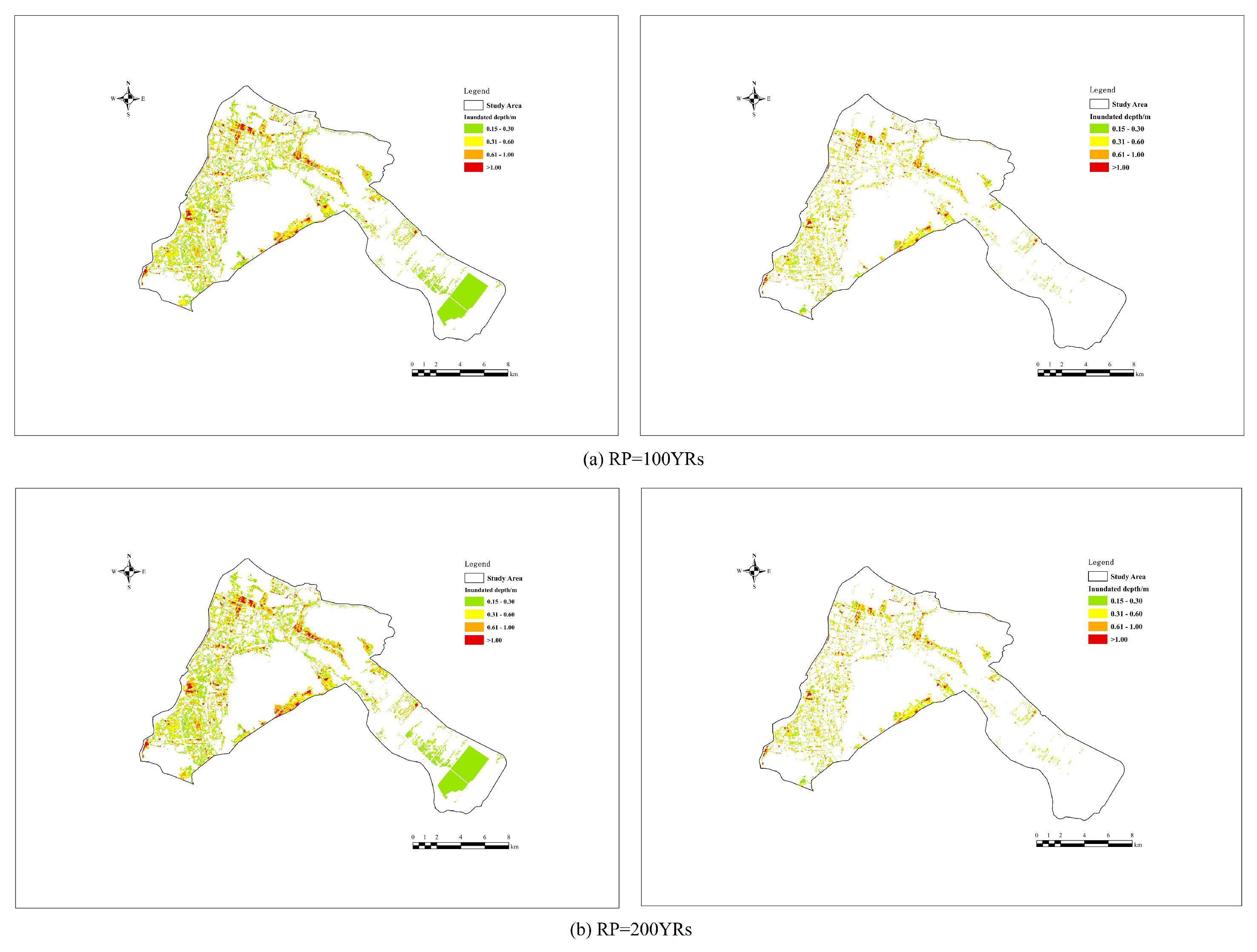
3.6. Compound Flooding Assessment

1.

Classification of flood hazard

In this part of the assessment, two distinct approaches were employed to generate flood hazard maps. The first approach is based on the joint probability distribution of three flood-related variables (total water level, discharge, and precipitation). The joint probability distribution of these three variables was considered, and the corresponding characteristic values for the same return period were calculated. These values were then used as boundary conditions in the hydrodynamic model for computation. The second approach relies on univariate frequency analysis, which only takes into account the frequency distributions of total water level, discharge, and precipitation. The boundary conditions for this method are the characteristic values corresponding to the return period of each single variable. For instance, the design values for total water level, discharge, and precipitation corresponding to a certain return period were identified and used as boundary conditions in the hydrodynamic model. Compared with the first approach, this method does not consider the joint probability distribution of the three variables when setting the boundary conditions. Therefore, under the same return period, the boundary conditions set in this approach are relatively conservative and may lead to a certain amplification effect. By comparing the flood hazard maps generated by the two methods, this part aims to identify the areas where the inundated depths are overestimated and/or underestimated.

In order to determine the inundation areas of the research region under various Compound Flooding (CF) scenarios and Univariate Frequency (UF) scenarios within the respective flood hazards, flood hazard categories were classified based on different inundated depths. The following five degrees of flood danger classification for urban flood events were suggested: (1) inundated depth greater than 1.0 m, which is regarded as an extremely high hazard and poses a threat to the safety of all pedestrians; (2) inundated depth between 0.6 and 1.0 m, where adult safety cannot be guaranteed, and work and production must be halted, which is regarded as a high hazard; (3) inundated depth between 0.3 and 0.6 m, which is regarded as a moderate hazard and could endanger children’s safety; (4) inundated depth between 0.15 and 0.3 m are regarded as lower hazards, but they have a substantial impact on residents’ mobility and vehicle safety; (5) Flood depths below 0.15 m are regarded as minor risks, where the standing water on the ground can quickly recede and have little effect on daily life and production.

2.

Quantification of the compound flood hazard

Table 10. Flood Hazards Results of Compound Flooding scenario and Univariate Frequency scenario.

Scenarios	Inundated Depth/m	Inundated Area/km2
		5a	10a	25a	50a	100a	200a
Compound Flooding scenario	0.15~0.30	16.30	20.67	24.50	25.78	27.92	30.43
	0.30~0.60	13.19	18.71	26.93	33.28	37.07	39.72
	0.60~1.0	4.38	7.56	11.98	16.30	20.42	25.11
	>1.0	1.01	2.21	4.19	6.29	8.11	9.81
	Total Area/km2	34.87	50.57	67.60	81.65	93.52	105.06
Univatiare Frequency scenario	0.15~0.30	14.18	16.47	19.82	22.35	24.61	24.55
	0.30~0.60	11.18	13.27	18.72	25.01	27.98	26.80
	0.60~1.0	3.66	4.53	6.69	10.27	12.94	11.92
	>1.0	0.84	1.07	1.92	3.43	4.67	4.21
	Total Area/km2	29.86	35.34	47.16	61.06	70.19	67.48

presents the flood hazard results for both the compound flooding scenario and the univariate frequency scenario. The study area’s flooding hazards for RPs = 100a and 200a were contrasted in Figure 9. In highly populated areas, the maximum inundation depths for the UF Scenario (RP = 200a, Figure 9b, right panel) and the CF Scenario (RP = 200a, Figure 9b, left panel) are 3.80 and 5.33 m, respectively. The maximum inundated depths for the UF Scenario (RP = 100a, Figure 9a, right panel) and the CF Scenario (RP = 100a, Figure 9a, left panel) are 3.61 and 4.88 m, respectively. This indicates that univariate frequency analysis can significantly underestimate flood peaks and hazards under extremely high return periods, especially in densely populated areas. The inundation comparison maps for return periods of 5a,10a,25a and 50a are shown in Figure 10.

Figure 11 presented a detailed analysis of the percentage increase in inundated areas for different RPs (5a, 10a, 25a, 50a, 100a, and 200a) and various inundated depths. Due to the limited intensity and extent of flooding at lower return periods (such as the 5a and 10a), the increase in inundated areas is relatively low across all inundated depths. This suggested that flood events are relatively common during these return periods, and traditional flood defense measures are sufficient to cope with them. However, as the return period increases, particularly at medium (such as 25a and 50a) and high return periods (such as 100a and 200a), there was a significant increase in the percentage of inundated area for depths greater than 0.30 m. This increase was especially pronounced in the 0.60–1.0 m and >1.0 m. For depths greater than 1.0 m, the increase reached as high as 133.02% at the 200a return period, underscoring the accuracy and importance of the compound flooding design in assessing flood hazards during extreme events.

3.

Calculation and assessment of amplification flood hazard

For flood events with different return periods (5, 10, 25, 50, 100, and 200a), this study used data fitting to examine the relationships between the ratios of precipitation (b₁), river discharge (b₂), and total water level (b₃) with the ratio of inundation areas (A₂/A₁) across three hazard levels (extremely high, high, and medium).

The effect of the optimized regression coefficients on the ratio of inundation areas was evaluated using data fitting. Equation (11) is the regression equation that results from the model’s R² of 0.80 and Standard Estimation Error (SEE) of 0.28 at the extreme high-hazard level. Equation (12) was obtained for the high-hazard level when the R² was 0.96 and the SEE was 0.10.

$${\displaystyle \frac{E{H}_{A_2}}{E{H}_{A_1}}}=0.95\times {\displaystyle \frac{P_2}{P_1}}+0.60\times {\displaystyle \frac{Q_2}{Q_1}}+0.75\times {\displaystyle \frac{Z_2}{Z_1}}-1.5$$

(28)

$${\displaystyle \frac{H_{A_2}}{H_{A_1}}}=0.95\times {\displaystyle \frac{P_2}{P_1}}+0.24\times {\displaystyle \frac{Q_2}{Q_1}}+0.75\times {\displaystyle \frac{Z_2}{Z_1}}-1.06$$

(29)

$${\displaystyle \frac{M_{A_2}}{M_{A_1}}}=0.33\times {\displaystyle \frac{P_2}{P_1}}+0.10\times {\displaystyle \frac{Q_2}{Q_1}}+0.40\times {\displaystyle \frac{Z_2}{Z_1}}+0.24$$

(30)

The weights of the amplification ratios for precipitation, discharge, and water level were assessed by comparing regression coefficients across various hazard levels and normalizing coefficients b₁, b₂, and b₃. The weights were 0.41, 0.26, and 0.33 under extreme high hazard, 0.49, 0.12, and 0.39 under high hazard, and 0.40, 0.12, and 0.48 under medium hazard. The results showed that the weight of the discharge amplification ratio (Q₂/Q₁) was the most significant at both extremely high and high-hazard levels. This suggests that the amplification of upstream river discharge has the most significant effect on changes in inundation regions at these hazard levels. On the other hand, the total water level amplification ratio (Z₂/Z₁) had the maximum weight at the medium-hazard level, suggesting that the amplification effect of water levels had the greatest impact on inundation areas in medium-hazard coastal zones.

The constant term m in the regression model typically represents the expected value of the dependent variable (A₂/A₁) when all variables (P₂/P₁, Q₂/Q₁, Z₂/Z₁) equal zero. In the context of flood hazard assessment, m signifies the baseline level of inundation area in the absence of changes in precipitation, river discharge, and water level. This study found that the constant term m varied significantly across hazard levels, suggesting that the impact of other factors on changes in inundation areas varies by hazard level: m = −1.5 for extreme high hazard, m = −1.06 for high hazard, and m = 0.24 for medium hazard. This suggests that, even in the absence of changes in precipitation, river discharge, and water level, the baseline level of inundation area ratio is negative for the extreme risk range, suggesting that other anthropogenic factors (e.g., effective drainage systems, good river management, and flood control facilities) have a significant positive effect in reducing flood risk areas. For high-hazard areas, even though the value of m increased, it remained negative, suggesting that these factors still have a positive impact, albeit to a lesser extent. For medium-hazard areas, m became positive, suggesting that the influence of these factors on medium-hazard inundation areas is relatively minor.

4. Discussions

4.1. Advancements in the Results

The integration of statistical and hydrodynamic models in this study has facilitated a comprehensive evaluation of compound flood hazards in coastal cities. Our approach involved fitting various distribution functions to precipitation, total water levels, and river discharge data, with the best-fitting distributions identified through rigorous goodness-of-fit tests. The application of Copula functions to construct bivariate and trivariate joint probability models further enhanced our ability to capture the complex statistical characteristics of compound flood events.

The calculation of flood return periods and design values revealed significant insights. The finding that joint return periods under the “OR” condition are lower than those under the “AND” condition highlights the higher frequency of concurrent flood characteristics in OR scenarios. This underscores the critical need to account for the coupling effects of multiple disaster factors in flood risk management. Moreover, the design values derived from the trivariate Copula functions were notably higher than those from univariate and bivariate probability distributions. This indicates that incorporating compound flood events into engineering design can substantially increase the safety margin. This finding is of paramount importance for enhancing the design standards of flood defense infrastructure in coastal cities, suggesting that traditional univariate design standards may be insufficient to ensure adequate protection against compound flood events.

The comparison of flood hazard maps generated from trivariate joint probability distributions and univariate frequency analyses further demonstrated the advantages of the compound flood design. The results showed that univariate frequency analysis can significantly underestimate flood peaks and hazard levels, particularly in high-return periods and densely populated areas. This highlights the necessity of considering compound flood events in flood hazard assessments and mitigation planning. The findings not only provide a new perspective for flood defense in coastal cities but also offer valuable insights for other regions affected by compound floods.

4.2. Amplification of Flood Hazards

The application of linear regression analysis in this study provided a detailed examination of how the amplification ratios of precipitation, river discharge, and total water level impact flood inundation areas. The analysis revealed significant variations in the weights of these factors across different hazard levels. For instance, at the extremely high hazard level, the amplification ratio of river discharge (Q2/Q1) had the highest weight, indicating its substantial influence on flood inundation areas. In contrast, at the high hazard level, the amplification ratio of precipitation (P2/P1) was the most significant, while at the medium hazard level, the amplification ratio of total water level (Z2/Z1) had the greatest impact. These findings emphasize the need for targeted flood risk reduction strategies that consider the specific hazard levels and influencing factors to achieve effective flood risk management. They also highlight the differential impact of these factors on flood inundation areas across various hazard levels, suggesting that a multifaceted approach is necessary when devising flood mitigation measures.

Further analysis of the constant term m in the regression model, which represents the baseline level of inundation area in the absence of changes in precipitation, river discharge, and water level, revealed notable differences across hazard levels. In extremely high-hazard areas, the significant positive impact of human factors such as effective drainage systems, good river management, and flood control facilities was evident, as indicated by the negative value of m. In high-hazard areas, although the positive impact of these factors was less pronounced, it still played a role in reducing flood risk. However, in medium-hazard areas, the influence of these factors on inundation areas was relatively minor. This underscores the varying influence of human factors on flood inundation areas across different hazard levels. It suggests that while robust drainage systems and flood control measures can significantly reduce flood risk in extremely high-hazard areas, their impact is more limited in medium-hazard areas. Therefore, a comprehensive approach that considers both natural and human factors is essential for effective flood risk management.

5. Conclusions

The present study proposed a comprehensive analysis of compound flooding hazards in Lianyungang City, Jiangsu Province, China, by examining the interactions between extreme precipitation events, maximum total water levels, and river discharge within a ±4-day interval. Through the application of univariate, bivariate, and trivariate statistical models and hydrodynamic modeling, the return periods and extreme values for univariate, bivariate, and trivariate flood events were quantified, and the amplification of flood hazards was evaluated. The major contributions of the presented work are:

• Copula Modeling and Optimal Distribution Functions: The Gamma distribution was found to best represent precipitation data, the Weibull distribution for tidal data, and the GEV distribution for discharge data. These distributions were selected based on their performance in goodness-of-fit tests, including the K-S test, AIC, and BIC. For bivariate joint distributions, the Clayton Copula was identified as the best fit for precipitation and total water levels, while the Gaussian Copula was preferred for total water levels and river discharge. The Frank Copula was the best fit for the joint distribution of precipitation and river discharge. In trivariate modeling, the Gumbel-Hougaard Copula was shown to be the best model, which captured the joint distribution of three flood drivers.
• Return Periods and Design Values: The return periods calculated for each flood driver and, in combination, show the increased frequency of compound flood events under “OR” conditions when compared to “AND” conditions. The design values derived from the trivariate copula functions provided a more conservative estimate of flood hazard, which is crucial for enhancing the safety margin in engineering design against extreme flood events.
• Compound Flooding Scenario Benefits: According to the simulation results obtained from the built hydrodynamic models, the proposed compound flooding design offered a comprehensive analysis of the flooding effects, particularly in high-hazard areas during medium to high return periods. Future flood hazard assessments and the development of flood mitigation plans should utilize the compound flooding design approach more. Future studies and practice should examine and optimize compound flooding design approaches to increase coastal communities’ resilience and adaptive capacity against compound flooding disasters.
• Amplification of Flood Hazards: A linear regression analysis tailored to various hazard levels was proposed to examine the amplification patterns of precipitation, river discharge, and total water level. The analysis indicated that the weight of these factors varies across hazard levels. At the medium-hazard level, the water level amplification ratio carried the highest weight, indicating that the impact of water level increases was most pronounced in the inundation of coastal areas classified as medium hazard.

References

1. Vousdoukas, M.I.; Mentaschi, L.; Voukouvalas, E.; Bianchi, A.; Dottori, F.; Feyen, L. Climatic and socioeconomic controls of future coastal flood risk in Europe. Nat. Clim. Change 2018, 8, 776–780. [Google Scholar]
2. Su, C.-W.; Song, Y.; Umar, M. Financial aspects of marine economic growth: From the perspective of coastal provinces and regions in China. Ocean. Coast. Manag. 2021, 204, 105550. [Google Scholar]
3. Athanasiou, P.; van Dongeren, A.; Pronk, M.; Giardino, A.; Vousdoukas, M.; Ranasinghe, R. Global Coastal Characteristics (GCC): A global dataset of geophysical, hydrodynamic, and socioeconomic coastal indicators. Earth Syst. Sci. Data 2024, 16, 3433–3452. [Google Scholar]
4. Lincke, D.; Hinkel, J. Coastal Migration due to 21st Century Sea-Level Rise. Earth’s Future 2021, 9, e2020EF001965. [Google Scholar]
5. Diermanse, F.; Roscoe, K.; Ormondt, M.; Leijnse, T.; Winter, G.; Athanasiou, P. Probabilistic compound flood hazard analysis for coastal risk assessment: A case study in Charleston, South Carolina. Shore Beach 2023, 91, 9–18. [Google Scholar]
6. Leijnse, T.; Goede, R.; Ormondt, M.; Lemans, M.; Hegnauer, M.; Eilander, D.; Kleermaeker, S.; Morales, Y.; Maguire, S. Developing Large Scale and Fast Compound Flood Models for Australian Coastlines. In Proceedings of the 37th Conference on Coastal Engineering, Sydney, Australia, 4–9 December 2022; p. 49. [Google Scholar]
7. Aziz, F.; Wang, X.; Mahmood, M.Q.; Awais, M.; Trenouth, B. Coastal urban flood risk management: Challenges and opportunities—A systematic review. J. Hydrol. 2024, 645, 132271. [Google Scholar]
8. Xu, H.; Zhang, X.; Guan, X.; Wang, T.; Ma, C.; Yan, D. Amplification of Flood Risks by the Compound Effects of Precipitation and Storm Tides Under the Nonstationary Scenario in the Coastal City of Haikou, China. Int. J. Disaster Risk Sci. 2022, 13, 602–620. [Google Scholar]
9. Latif, S.; Simonovic, S.P. Compounding joint impact of rainfall, storm surge and river discharge on coastal flood risk: An approach based on 3D fully nested Archimedean copulas. Environ. Earth Sci. 2023, 82, 63. [Google Scholar]
10. Comer, J.; Olbert, A.I.; Nash, S.; Hartnett, M. Development of high-resolution multi-scale modelling system for simulation of coastal-fluvial urban flooding. Nat. Hazards Earth Syst. Sci. 2017, 17, 205–224. [Google Scholar]
11. Olbert, A.I.; Comer, J.; Nash, S.; Hartnett, M. High-resolution multi-scale modelling of coastal flooding due to tides, storm surges and rivers inflows. A Cork City example. Coast. Eng. 2017, 121, 278–296. [Google Scholar]
12. Lin, Q.; Shi, L.; Liang, B.; Wu, G.; Wang, Z.; Zhang, X.; Wu, Y. Characterizing interactive compound flood drivers in the Pearl River Estuary: A case study of Typhoon Hato (2017). J. Hydrol. 2024, 645, 132270. [Google Scholar]
13. Tilloy, A.; Malamud, B.D.; Winter, H.; Joly-Laugel, A. A review of quantification methodologies for multi-hazard interrelationships. Earth-Sci. Rev. 2019, 196, 102881. [Google Scholar]
14. Tilloy, A.; Malamud, B.D.; Winter, H.; Joly-Laugel, A. Evaluating the efficacy of bivariate extreme modelling approaches for multi-hazard scenarios. Nat. Hazards Earth Syst. Sci. 2020, 20, 2091–2117. [Google Scholar]
15. Archer, L.; Neal, J.; Bates, P.; Lord, N.; Hawker, L.; Collings, T.; Quinn, N.; Sear, D. Population exposure to flooding in Small Island Developing States under climate change. Environ. Res. Lett. 2024, 19, 124020. [Google Scholar]
16. John, A.; Bhagyanathan, A.; Parvin Cm, K. Framework for urban flood risk assessment—A hydrological modelling approach: The case of Nilambur, Kerala. Int. Plan. Stud. 2024, 29, 342–365. [Google Scholar]
17. Cánovas-García, F.; Vargas Molina, J. An exploration of exposure to river flood risk in Spain using the National Floodplain Mapping System. Geomat. Nat. Hazards Risk 2025, 16, 2421405. [Google Scholar] [CrossRef]
18. Zscheischler, J.; Westra, S.; van den Hurk, B.J.J.M.; Seneviratne, S.I.; Ward, P.J.; Pitman, A.; AghaKouchak, A.; Bresch, D.N.; Leonard, M.; Wahl, T.; et al. Future climate risk from compound events. Nat. Clim. Change 2018, 8, 469–477. [Google Scholar]
19. Bevacqua, E.; Vousdoukas, M.I.; Shepherd, T.G.; Vrac, M. Brief communication: The role of using precipitation or river discharge data when assessing global coastal compound flooding. Nat. Hazards Earth Syst. Sci. 2020, 20, 1765–1782. [Google Scholar]
20. Wahl, T.; Jain, S.; Bender, J.; Meyers, S.D.; Luther, M.E. Increasing risk of compound flooding from storm surge and rainfall for major US cities. Nat. Clim. Change 2015, 5, 1093–1097. [Google Scholar]
21. Xu, H.; Xu, K.; Bin, L.; Lian, J.; Ma, C. Joint Risk of Rainfall and Storm Surges during Typhoons in a Coastal City of Haidian Island, China. Int. J. Environ. Res. Public Health 2018, 15, 1377. [Google Scholar] [CrossRef]
22. Ward, P.J.; Couasnon, A.; Eilander, D.; Haigh, I.D.; Hendry, A.; Muis, S.; Veldkamp, T.I.E.; Winsemius, H.C.; Wahl, T. Dependence between high sea-level and high river discharge increases flood hazard in global deltas and estuaries. Environ. Res. Lett. 2018, 13, 084012. [Google Scholar] [CrossRef]
23. Inamdeen, F.; Larson, M. Compound effects of sea level and flow on river-induced flooding in coastal areas of southern Sweden. J. Hydrol. Reg. Stud. 2024, 56, 102032. [Google Scholar] [CrossRef]
24. Wang, Z.; Chen, Y.; Zeng, Z.; Li, R.; Li, Z.; Li, X.; Lai, C. Compound effects in complex estuary-ocean interaction region under various combination patterns of storm surge and fluvial floods. Urban Clim. 2024, 58, 102186. [Google Scholar] [CrossRef]
25. Bevacqua, E.; De Michele, C.; Manning, C.; Couasnon, A.; Ribeiro, A.F.S.; Ramos, A.M.; Vignotto, E.; Bastos, A.; Blesić, S.; Durante, F.; et al. Guidelines for Studying Diverse Types of Compound Weather and Climate Events. Earth’s Future 2021, 9, e2021EF002340. [Google Scholar] [CrossRef]
26. Latif, M.; Firuza, M. Parametric Vine Copula Construction for Flood Analysis for Kelantan River Basin in Malaysia. Civ. Eng. J. 2020, 6, 1470–1491. [Google Scholar] [CrossRef]
27. Fang, J.Y.; Yin, J.; Shi, X.W.; Fang, J.; Du, S.Q.; Liu, M. A review of compound flood hazard research in coastal areas. Adv. Clim. Change Res. 2021, 17, 317–328. [Google Scholar]
28. Couasnon, A.; Sebastian, A.; Morales-Nápoles, O. A Copula-Based Bayesian Network for Modeling Compound Flood Hazard from Riverine and Coastal Interactions at the Catchment Scale: An Application to the Houston Ship Channel, Texas. Water 2018, 10, 1190. [Google Scholar] [CrossRef]
29. Bass, B.; Bedient, P. Surrogate modeling of joint flood risk across coastal watersheds. J. Hydrol. 2018, 558, 159–173. [Google Scholar] [CrossRef]
30. Santiago-Collazo, F.L.; Bilskie, M.V.; Bacopoulos, P.; Hagen, S.C. Compound Inundation Modeling of a 1-D Idealized Coastal Watershed Using a Reduced-Physics Approach. Water Resour. Res. 2024, 60, e2023WR035718. [Google Scholar] [CrossRef]
31. Muñoz, D.F.; Moftakhari, H.; Moradkhani, H. Compound Effects of Flood Drivers and Wetland Elevation Correction on Coastal Flood Hazard Assessment. Water Resour. Res. 2020, 56, e2020WR027544. [Google Scholar] [CrossRef]
32. Serafin, K.A.; Ruggiero, P.; Parker, K.; Hill, D.F. What’s streamflow got to do with it? A probabilistic simulation of the competing oceanographic and fluvial processes driving extreme along-river water levels. Nat. Hazards Earth Syst. Sci. 2019, 19, 1415–1431. [Google Scholar] [CrossRef]
33. Liu, B.; Xu, S.; Yin, K. Spatial inhomogeneity analyses of extreme sea levels along Lianyungang coast based on numerical simulation and Monte Carlo model. Reg. Stud. Mar. Sci. 2024, 79, 103856. [Google Scholar] [CrossRef]
34. Xu, H.; Xu, K.; Lian, J.; Ma, C. Compound effects of rainfall and storm tides on coastal flooding risk. Stoch. Environ. Res. Risk Assess. 2019, 33, 1249–1261. [Google Scholar] [CrossRef]
35. Akaike, H. A new look at the statistical model identification. IEEE Trans. Autom. Control 1974, 19, 716–723. [Google Scholar] [CrossRef]
36. Schwarz, G. Estimating the Dimension of a Model. Ann. Stat. 1978, 6, 461–464. [Google Scholar] [CrossRef]
37. Chu, H.-J.; Lin, Y.-P.; Huang, C.-W.; Hsu, C.-Y.; Chen, H.-Y. Modelling the hydrologic effects of dynamic land-use change using a distributed hydrologic model and a spatial land-use allocation model. Hydrol. Process. 2010, 24, 2538–2554. [Google Scholar] [CrossRef]
38. Dwarakish, G.S.; Ganasri, B.P. Impact of land use change on hydrological systems: A review of current modeling approaches. Cogent Geosci. 2015, 1, 1115691. [Google Scholar] [CrossRef]
39. Sun, Y.; Liu, C.; Du, X.; Yang, F.; Yao, Y.; Soomro, S.-E.-H.; Hu, C. Urban storm flood simulation using improved SWMM based on K-means clustering of parameter samples. J. Flood Risk Manag. 2022, 15, e12826. [Google Scholar] [CrossRef]
40. Zhu, W.; Cao, Z.; Kawaike, K.; Luo, P.; Yamanoi, K.; Koshiba, T. A novel urban flood risk assessment framework based on refined numerical simulation technology. J. Hydrol. 2024, 645, 132152. [Google Scholar] [CrossRef]
41. Gallien, T.W.; Kalligeris, N.; Delisle, M.-P.C.; Tang, B.-X.; Lucey, J.T.D.; Winters, M.A. Coastal Flood Modeling Challenges in Defended Urban Backshores. Geosciences 2018, 8, 450. [Google Scholar] [CrossRef]
42. Cai, H.; Yang, Q.; Zhang, Z.; Guo, X.; Liu, F.; Ou, S. Impact of River-Tide Dynamics on the Temporal-Spatial Distribution of Residual Water Level in the Pearl River Channel Networks. Estuaries Coasts 2018, 41, 1885–1903. [Google Scholar] [CrossRef]
43. Williams, L.L.; Lück-Vogel, M. Comparative assessment of the GIS based bathtub model and an enhanced bathtub model for coastal inundation. J. Coast. Conserv. 2020, 24, 23. [Google Scholar] [CrossRef]
44. Kouakou, M.; Tiémélé, J.A.; Djagoua, É.; Gnandi, K. Assessing potential coastal flood exposure along the Port-Bouët Bay in Côte d’Ivoire using the enhanced bathtub model. Environ. Res. Commun. 2023, 5, 105001. [Google Scholar] [CrossRef]
Figure 1. Maps illustrating the study area (a) Global location of the Central City District of Lianyungang within Jiangsu Province, China. (b) Detailed depiction of the study area, highlighting primary hazard sources and gauging stations. The Qiangwei River, significant as upstream discharge, is represented with a bold blue line. Total water levels from the Yellow Sea, which represent downstream high tide, are indicated by a blue wave pattern, and precipitation areas are marked in a darker blue color. Additionally, gauging stations for rainfall, streamflow and tide levels are marked with red dots, green squares, and triangles, respectively. The locations of these stations, including their latitudes and longitudes, are detailed in Table 1.
Land 14 00816 g001
Figure 2. Methodological framework for compound flood disaster assessment in this study.
Land 14 00816 g002
Figure 3. 1D Model domain of Central City District. (a) 1D river network hydrodynamic model. (b) 1D pipeline network model.
Land 14 00816 g003
Figure 4. 1D and 2D Coupled Flood Propagation Model Domain of Central City District. (a) 1D-2D Coupled model construction. (b) Connection details.
Land 14 00816 g004
Figure 5. Calibration of simulated water levels of rainfall process on 6~9 July 2024: (a) Riverside Park, (b) Phoenix Mouth, (c) Yudai River, (d) Longwei River.
Land 14 00816 g005
Figure 6. Calibration of simulated water levels of rainfall process on 26~29 August 2023: (a) Riverside Park. (b) Phoenix Mouth, (c) Dapu Branch River.
Land 14 00816 g006
Figure 7. Univariate CDFs (Lognormal, Gamma, Weibull, GEV, and Normal) with corresponding P-P plots and Q-Q plots.
Land 14 00816 g007
Figure 8. Design scheme boundaries for varing RPs.
Land 14 00816 g008
Figure 9. Comparison of lnundated Depths for Different RPs under Two Scenarios, with the Left Panel Representing the Compound Flooding Scenario and the Right Panel Representing Univariate Frequency Analysis. (a) Return Period = 100 yrs; (b) Return Period = 200 yrs.
Land 14 00816 g009
Figure 10. Comparison of lnumdated Depths for Different RPs under Two Scenarios, with the Left Panel Representing the Compound Flooding Scenario and the Right Panel Representing Univariate Frequency Analysis. (a) Return Period = 5 yrs; (b) Return Period = 10 yrs; (c) Return Period = 25 yrs; (d) Return Period = 50 yrs.
Land 14 00816 g010
Figure 11. Analysis of the Percentage Increase in Inundated Area under Different RPs.
Land 14 00816 g011