Article

Power Spectra’s Perspective on Meteorological Drivers of Snow Depth Multiscale Behavior over the Tibetan Plateau

1
School of Transportation and Civil Engineering, Nantong University, Nantong 226019, China
2
State Key Laboratory of Remote Sensing and Digital Earth, Faculty of Geographical Science, Beijing Normal University, Beijing 100875, China
*
Author to whom correspondence should be addressed.
Land 2025, 14(4), 790; https://doi.org/10.3390/land14040790
Submission received: 5 March 2025 / Revised: 1 April 2025 / Accepted: 3 April 2025 / Published: 7 April 2025

Abstract

:
The meteorology-driven multiscale behavior of snow depth over the Tibetan Plateau was investigated via analyzing the spatio-temporal variability of snow depth over 28 intraseasonal continuous snow cover regions. By employing power spectra and the Kullback–Leibler (K-L) distance, the spectral similarities between snow depth and meteorological factors were examined at scales of 5 km, 10 km, 20 km, and 50 km across seasons from 2008 to 2014. Results reveal distinct seasonal and scale-dependent dynamics: in spring and winter, snow depth exhibits lower spectral variance with scale breaks around 50 km, emphasizing the critical roles of precipitation, atmospheric moisture, and temperature, with lower K-L distances at smaller scales. Summer shows the highest spatial variance, with snow depth primarily influenced by wind and radiation, as indicated by lower K-L distances at 15–45 km. Autumn demonstrates the lowest spatial heterogeneity, with windspeed driving snow redistribution at finer scales. The alignment between spatial variance maps and power spectra implies that snow depth data can be effectively downscaled or upscaled without significant loss of spatial information. These findings are essential for improving snow cover modeling and forecasting, particularly in the context of climate change, as well as for effective water resource management and climate adaptation strategies in this strategically vital plateau.

1. Introduction

The Tibetan Plateau (TP), often heralded as the “Third Pole,” represents one of the Earth’s most significant and sensitive climatic and hydrological regions. Encompassing the largest reservoir of ice and snow outside the polar regions, the TP exerts a profound influence on atmospheric circulation and climate patterns both regionally and globally [1]. The plateau’s snow cover regulates seasonal water availability by controlling river discharge patterns, sustaining hydropower, and influencing groundwater recharge. Variability in snow depth affects water resources by altering the timing and magnitude of runoff, increasing the risk of droughts and floods in downstream regions that depend on glacial and snow-fed rivers. These hydrological shifts have cascading effects on biodiversity, as alpine ecosystems adapted to stable snow conditions face disruptions in habitat availability and food supply. Additionally, local communities that rely on snow-dependent activities such as agriculture, livestock grazing, and winter tourism experience economic challenges due to inconsistent snow cover. The plateau’s extensive snowpack also plays a crucial role in the Asian monsoon system, affecting billions of people downstream [2]. Moreover, the snowpack on the TP is a critical source of water for many of Asia’s major river systems, including the Yangtze, Yellow, Indus, and Mekong, underscoring its importance in regional water security and ecosystem services [3,4,5]. However, the TP is experiencing rapid environmental changes, with implications for snow depth (SD) variability and distribution that are not yet fully understood [6]. The dynamics of snow depth on the TP, influenced by a complex interplay of meteorological controls such as temperature [7], precipitation [8], wind patterns [9], and atmospheric circulation [10,11] highlight the sensitivity of the TP’s snow cover to climatic fluctuations and underscore the importance of understanding the underlying meteorological controls.
Advancements in remote sensing and in situ measurements have shed light on these complex interactions, revealing the challenges in snow monitoring tied to coarse resolution [12,13] and emphasizing the necessity for integrating multiple data sources [14]. Specifically, fusing passive microwave snow depth data with optical snow cover data at high temporal resolution can enhance the spatial granularity of snow depth measurements, and provide a more nuanced understanding of snow distribution patterns across the plateau [15]. In a complementary vein, Gao et al. [16] discerned the contributions of the longest snow cover duration and short-term snow cycles to the annual snow cover days, and unveiled the intricate mosaic of regional snow cover dynamics. Similarly, integrating optical snow extent products into brightness temperature datasets, downscaled snow depth data achieved high accuracy and spatio-temporal heterogeneity [17,18].
The scale behavior of snow depth, shaped by meteorological controls, is fundamental to understanding its variability across spatial and temporal domains. Snow depth exhibits pronounced multiscale characteristics, influenced by local to regional factors such as vegetation, topography, wind redistribution, and synoptic weather patterns [19]. At finer spatial scales, variations in terrain and land cover create localized heterogeneity in snow accumulation and ablation, while at broader scales, large-scale atmospheric circulation and elevation gradients drive systematic snow distribution patterns. Temporally, snow depth fluctuations operate across multiple timescales, from daily weather events to seasonal cycles and interannual climate variability. Elevation-dependent warming introduces additional complexity, with its effects varying across different altitudes [20]. Seasonal snow patterns show distinct trends, with long-term variations following linear trajectories [21], while interannual fluctuations, particularly in late winter, are strongly influenced by changes in the intensity and position of westerly jet streams [22]. Given these complexities, traditional methods often struggle to capture the full spectrum of snow variability across scales. Power spectrum analysis provides a robust framework for identifying scale-dependent behaviors by quantifying how variance is distributed across spatio-temporal frequencies. This approach enables the detection of scaling breaks, which signify transitions in dominant snow depth drivers, and facilitates the differentiation between meteorological controls acting at different scales, contributing to improved snow modeling and prediction [23,24]. Although the spectral approach has been widely applied to analyze snow depth variability in other mountainous regions, including the Pyrenees [25] and the Bridger Range [26], studies utilizing these methods on the TP remain scarce. Given the TP’s complex meteorological influences on snow depth, applying power spectrum analysis provides a unique opportunity to systematically examine its multiscale meteorology-dependent snow dynamics via multisource data, addressing a significant gap in the existing literature.
By integrating power spectrum analysis and the Kullback–Leibler distance, this study offers a novel perspective on how meteorological factors regulate snow depth variability across different spatial scales. Unlike conventional approaches that primarily focus on mean snow depth trends, our method captures scale-dependent influences, revealing how factors such as wind speed, radiation, and humidity shape snow distribution at varying resolutions. Bridging the coarse resolution of conventional snow monitoring with the fine-scale snow depth heterogeneity, this endeavor holds profound implications for predicting future snow cover trends, managing water resources effectively, and formulating strategies for climate change adaptation in this strategically important region [27]. By isolating and analyzing atmospheric factors, rather than topographic influences, the study is centered on understanding the dynamic meteorology–snow interactions and offering essential insights for improving predictive models of snow behavior in response to climatic changes.

2. Materials and Methods

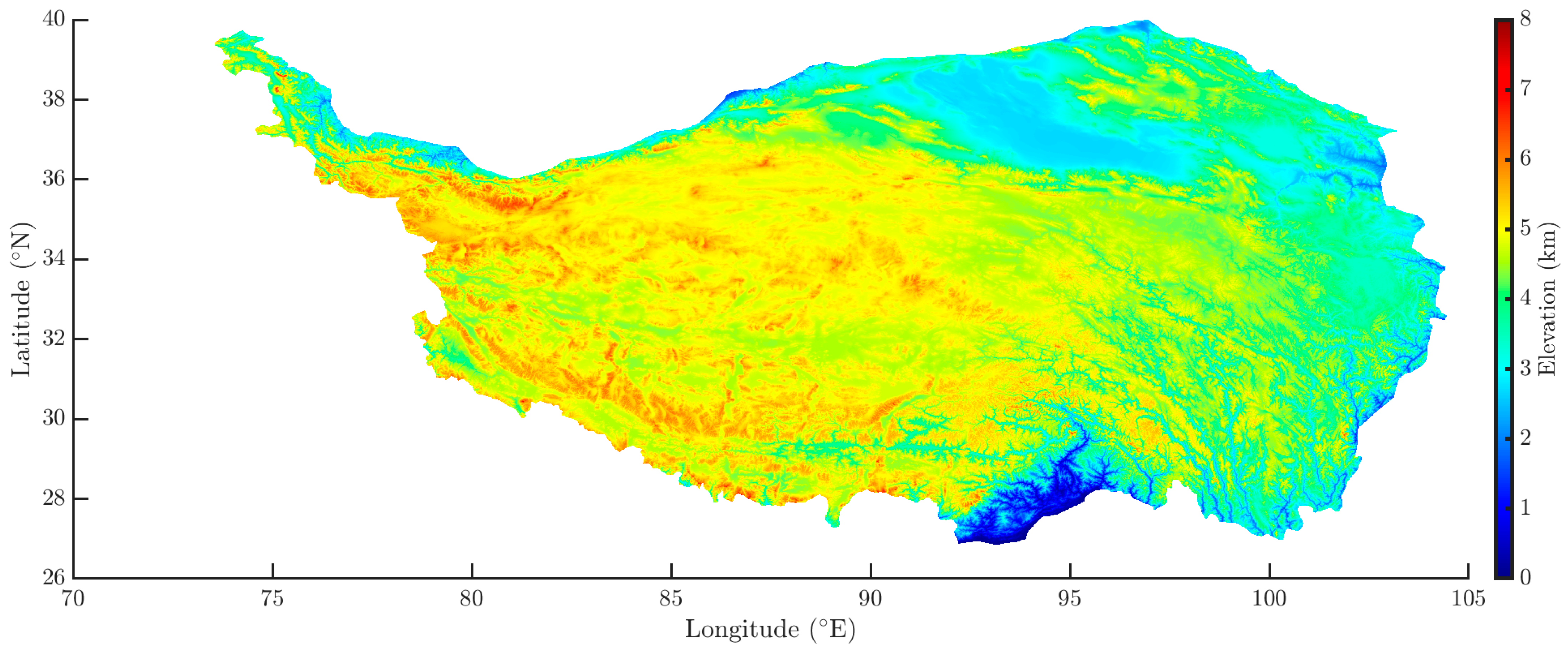
2.1. Tibetan Plateau

As the highest and vastest plateau in the world, the Tibetan Plateau (26°N–40°N, 70°E–105°E) covers approximately 2.5 million square kilometers. The elevation map (Figure 1) visualizes the intricate elevation patterns: the plateau is characterized by dramatic elevation gradients, with altitudes ranging from approximately 2000 m in the southeastern river valleys to peaks soaring above 8000 m.
The plateau encompasses a diverse range of topographical features and climatic conditions that contribute to various snow depth and meteorological patterns, making it an ideal location for studying the interplay between meteorological controls and snow dynamics. Thus, this study identified the 28 largest intraseasonal continuous snow cover regions (ICSCRs, Table 1), defined as regions where snow depth remains positive throughout an entire season, spanning 4 seasons—spring (March, April, May), summer (June, July, August), autumn (September, October, November), and winter (December, January, February)—across 7 years over the Tibetan Plateau. Each ICSCR represents a unique combination of local topographical and meteorological conditions; it also provides the necessary spatio-temporal consistency required to accurately investigate the multiscale behavior of snow depth.

2.2. Snow Depth Product

Coarser resolution datasets, such as those at multi-kilometer scales (e.g., 25 km), often fail to represent the intricate topographical and meteorological influences on snow depth, particularly in regions with complex terrain and heterogeneous climatic conditions like the TP.
Contrary to that, this study employed a daily 0.05° SD product [28] which was generated via spatio-temporally downscaling daily SD data and 8-day cloud-free snow cover probability data [14]. As validated by station records, the mean RMSE (root mean squared error) and MAE (mean absolute error) of the product are 1.54 and 0.67 cm/d, respectively [14]. This allows for enhanced spatial detail and capturing subtle variations in snow depth, as well as facilitating a more granular scale analysis (5–50 km) to identify how meteorological factors influence snow depth from local to regional scales.

2.3. Meteorological Reanalysis

Yang et al. [29] produced the TPMFD—a high-resolution (1/30°, hourly to monthly) near-surface meteorological forcing (2 m air temperature, precipitation, air pressure, incoming shortwave and longwave radiation, wind speed, and specific humidity) dataset for the Third Pole region. Precipitation, air temperature, specific humidity, and air pressure were derived by integrating high-resolution short-term WRF simulations, long-term ERA5 data, and site observations. Shortwave radiation was obtained by fusing ERA5 reanalysis data with satellite-derived shortwave radiation. Longwave radiation was calculated through the semi-physical CD99 model which utilizes other meteorological variables (air temperature, specific humidity, air pressure, and shortwave radiation).
The dataset offers higher precision compared to the current prevailing reanalysis ones. For example, regarding to 197 independent rain gauges, the precipitation has a 5 mm/d RMSE, a 0.76 correlation coefficient, and a 0.61 critical success index [30]. This study employed the monthly TPMFD data (average of the daily ones) to explore the meteorology-dependent multiscale behavior of snow depth over the TP. The selection of key meteorological variables—air temperature, specific humidity, downward shortwave radiation, wind speed, and precipitation—was because of their fundamental roles in controlling snow accumulation, metamorphism, and ablation processes. Air temperature governs the phase state of precipitation and the rate of snowmelt, while specific humidity influences deposition, sublimation, and condensation processes within the snowpack. Shortwave radiation serves as a primary energy source driving snowmelt, whereas wind speed affects redistribution, sublimation rates, and surface roughness, altering snowpack structure. Precipitation is the primary input to snow accumulation, with variations in its intensity and phase influencing snow depth fluctuations.

2.4. Scaling Analysis

Following Cao and Barros [31], scaling analysis which decomposed the spatial distribution of snow depth into its frequency components was performed to quantify the snow depth variability across scales. Specifically, the power spectral density was computed using a fast Fourier transform on the snow depth fields. The spectral slope was analyzed to assess the spatial heterogeneity, where a steeper slope indicates a more uniform distribution, while deviations from linearity suggest scale-dependent influences of meteorological drivers. The power spectra of snow depth and meteorological fields E k 2 ( k is wavenumber) can be calculated as follows:
E k 2 = C k β
where C is a constant, and spectral slope β between two scales (wavenumbers) was estimated by applying the log transform over the above equation:
β Δ log E k 2 Δ log k
Hypothetically, variations in spectral slope (i.e., scaling break) between adjacent scales indicate alterations in snow depth, as well as the attributed meteorological factors. Monotonic scaling behavior (constant β ) between two scales illustrates that the fields at smaller scales can be upscaled to larger scales via fractal upscaling while preserving the spatial statistical structure of the information at a higher resolution, and vice versa [32,33].
The power spectrum analysis offers valuable insights into the scale-dependent behavior of snow depth over the TP, which is crucial for understanding the complex interactions between snow cover and climate systems [34]. This approach enables the identification of dominant scales of variability and potential scale breaks influenced by meteorological factors.

2.5. Kullback–Leibler Distance

The Kullback–Leibler (K-L) distance D K L is used to quantify the similarity (small value) or divergence (large value) in the spectral characteristics of snow depth and meteorological variables across different scales. This approach allows for identifying the most influential meteorological factors on snow depth variability over the TP. D K L was calculated between the power spectrum curves of snow depth and those of seven meteorological variables, as well as among the meteorological forcings themselves:
D K L P , Q = 1 2 s P s log P s Q s + Q s log Q s P s
where P and Q are the two normalized power spectra to be evaluated, and s is the scale applied for the spectra. The distance captures the detailed difference in the scale domain due to taking the entire distribution including the tails into account. This method enhances the robustness of the analysis by focusing on spectral properties, which are often more informative than time-domain characteristics alone [35,36]. However, it is noteworthy that low K-L divergence indicates similarity in the shapes of spectral distributions but does not imply correlation, causation, or the direction of influence between variables. Such similarity could arise from coincidental distribution shapes or external common factors (e.g., seasonality) rather than a direct relationship. Alternative metrics, such as the Pearson correlation for linear dependencies or mutual information for broader associations, could complement this approach to assess true relational dependencies, though our focus here remains on scale-dependent spectral characteristics.

3. Results

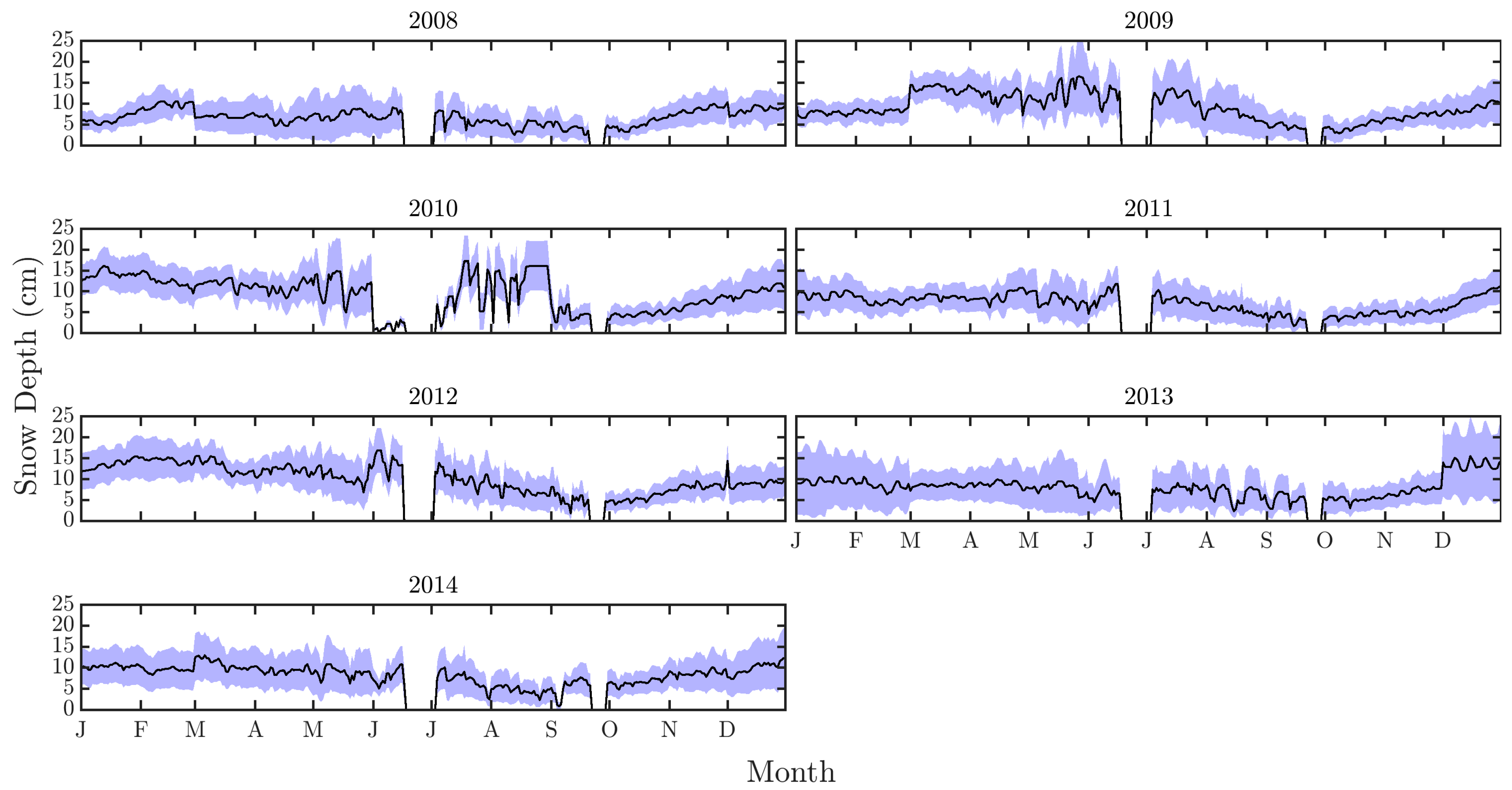
3.1. Spatio-Temporal Variations

Figure 2 and Figures S1–S7 present the time series of snow depth and seven meteorological factors across different ICSCRs and seasons over the years 2008 to 2014. Peak snow depths occur between December and January, with higher variability in 2014 indicating frequent snowfall events or prolonged snow cover [37,38] that can be attributed to the enhanced precipitation (Figure S5) and colder temperatures (Figure S7), particularly in ICSCRs located in the central and western high plains and mountain ranges. In contrast, the east plateau marked by a series of steep river gorges, such as the Yarlung Tsangpo River region, exhibits greater variability in snow depth (e.g., 2013 winter in Figure 2) due to distinct precipitation patterns and higher temperatures.
Moreover, Che et al. [39] and Pu et al. [40] reported similar seasonal dynamics in the TP, where specific humidity, radiation, and wind considerably influence snow cover variability. Figure S1 displays the consistent patterns of specific humidity peaking during the summer months, aligning with the monsoon season and impacting snow accumulation and melting phases. Similarly, the variations in longwave and shortwave radiation across different ICSCRs underline the role of solar and thermal radiation in snowmelt processes, particularly during the summer of 2010 and 2011 (see the western geolocations in Table 1), when elevated radiation levels were observed. Increased wind speed, particularly during winter, suggests the potential role of wind-induced snow transport in redistributing snow, contributing to spatial variability in snow depth within ICSCRs.

3.2. Power Spectra

The power spectra of snow depth and seven meteorological forcings, as presented in Figure 3 and Figures S8–S14, offer a comprehensive view of the multiscale spatial variability across the TP in different seasons, as well as the underlying meteorological controls. The spring and winter spectra stand out with their lower variabilities and slight scale breaks around 50 km, revealing a more homogeneous large-scale snow cover during the TP’s coldest months. The concurrent patterns of specific humidity (at lowest) and precipitation spectra emphasize that cold, dry conditions and snowfall favor snow preservation over the TP [41,42], enhancing predictability at regional scales due to strong, uniform meteorological signals. Furthermore, the straight spectra of air pressure and temperature display similar steady declines with occasional fluctuations, suggesting the stabilizing effect of high-pressure synoptic systems and persistent cold temperatures on the snow phenology through melting cycles [43,44]. The spectra of downward shortwave and longwave radiation present a uniform decline with minimal fluctuations, implying their combined influences on winter snow accumulation and melting rates [45].
In contrast, summer and autumn exhibit higher variances in the snow spectra, with relatively smooth declines across wavelengths, as well as scale breaks around 20 km and 50 km. This reflects the reduced snow cover and the dominance of smaller-scale processes such as localized melting and sublimation during the warm season [46], offering predictability at intermediate scales. Notably, specific humidity and wind reach their peaks also with scale breaks around 20 km and 50 km, implying the compound effects on snow redistribution and sublimation [47], which may complicate finer forecasts. Also, the spectra show rising variability at larger scales (longer wavelengths), which might be explained by the climatic transition and the commencement of the accumulation season [24]. This seasonal shift can influence the spatio-temporal distribution of snow depth, further affected by the plateau’s diverse terrain [48].

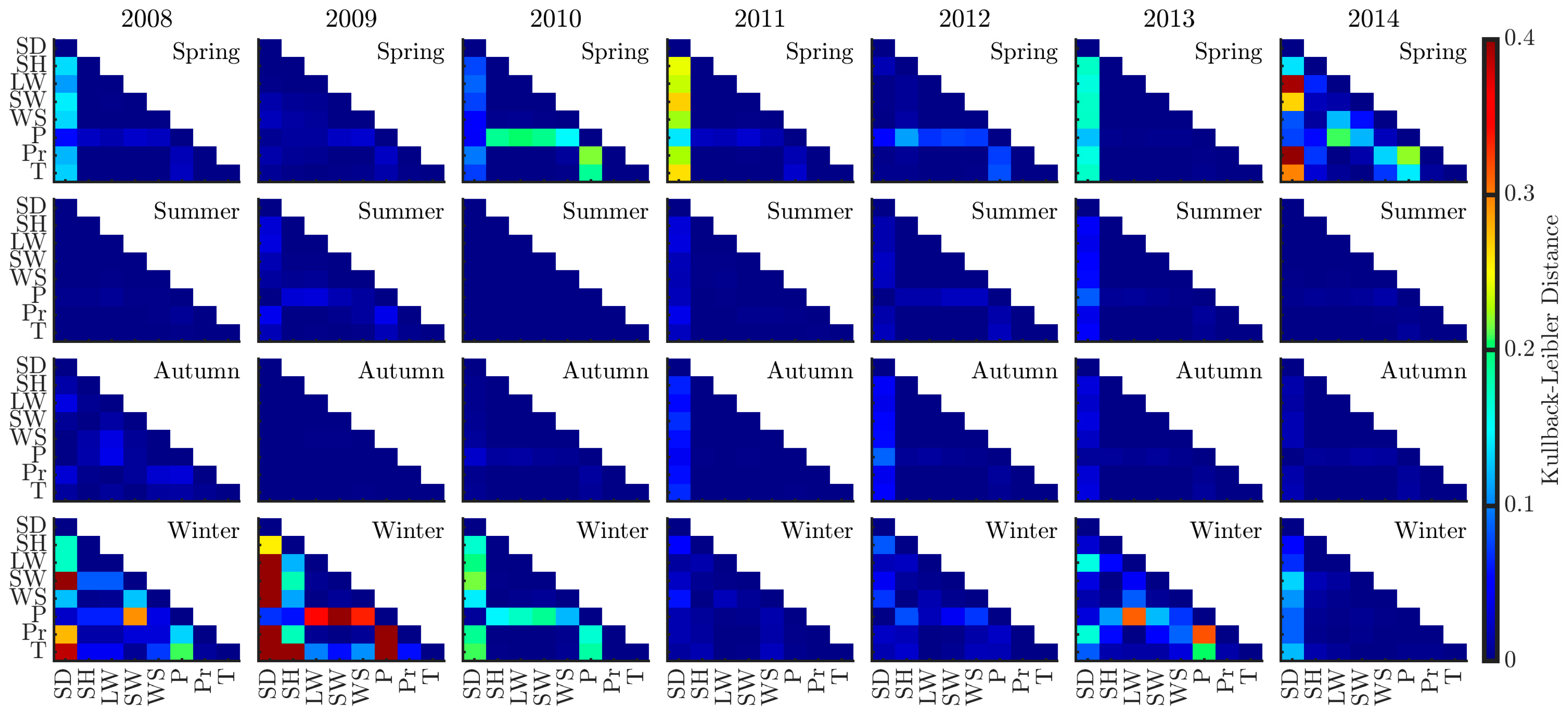
3.3. Spectral Divergence

Figure 4, Figures S15 and S16 illustrate D K L between the power spectra of snow depth ( S D ) and various meteorological forcings—specific humidity ( S H ), longwave radiation ( L W ), shortwave radiation ( S W ), precipitation ( P ), air pressure ( P r ), windspeed ( W S ), and temperature ( T ) over different seasons from 2008 to 2014 at 15–45 km, 15–30 km, and 30–45 km, respectively.
Across all scales, D K L demonstrates noticeable seasonal variation. In spring and winter, D K L exhibits more variability, particularly with W S , S H , and T , whose pronounced fluctuations were observed in 2011 and 2013. This underscores the importance of wind-induced moisture and heat transfer modulating snow dynamics [49]. The low D K L values at the 15–30 km scale demonstrate the homogeneous localized meteorological controls (e.g., P and T ) on snow depth during these seasons. This coherence diminishes at wider scales (15–45 km and 30–45 km), where diverse topographic and microclimatic conditions create heterogeneity in snow–meteorology interactions. As larger areas encompass different elevations and terrain types, snow depth variability becomes more spatially complex, which is less synchronized with broad-scale meteorological drivers [50].
Conversely, during summer and autumn, D K L remains relatively low throughout the years at 15–45 km, elucidating a more coherent, synchronized pattern across this broader range between snow depth and associated meteorological factors (e.g., S W and L W ), as well as the consistent influences on snow depth. The regularity of these relationships points to stable broad-scale meteorological controls over gradual snow accumulation and melt processes during these transitional seasons, which are corroborated by Qiao et al. [51] and Xu et al. [52]. However, at narrower scales (15–30 km and 30–45 km), the higher D K L implies increased divergence between snow depth and meteorological forcings. This suggests that regional processes become more pronounced when examining smaller spatial intervals. In summer, for instance, localized radiation-driven melting is not uniformly distributed across the landscape; these processes create spatial heterogeneity at finer resolutions. Similarly, in autumn, small-scale variations in T can cause snow depth patterns to vary significantly within these narrower scales, resulting in higher D K L . This divergence emphasizes the spatial variability introduced by localized meteorological dynamics that become salient when analyzing smaller scale ranges.

3.4. Spatial Heterogeneity Across Scales

As highlighted by seasonal D K L across snow depth and meteorological factors, four specific seasons (2011 spring, 2012 summer, 2013 autumn, and 2010 winter) were chosen to examine if the spatial heterogeneities of upscaled products (5 km, 10 km, 20 km, and 50 km) mapped by Figure 5 and Figures S17–S23 follow the corresponding spectra behavior.
In 2011 spring and 2010 winter, the snow depth showed moderate spatial variability, particularly at finer scales. For 2011 spring, the mean snow depth increased from 8.49 cm (STD = 3.29 cm) at 5 km to 8.62 cm (STD = 2.26 cm) at 50 km; for 2010 winter, it decreased from 12.17 cm (STD = 3.3 cm) at 5 km to 11.58 cm (STD = 2.36 cm) at 50 km, which embodies the scale breaks around 50 km in the two spectra. Specific humidity, precipitation, and air temperature exhibit similar spatial patterns, whose alignment with the power spectra implies that fine-scale variations in atmospheric moisture and temperature play crucial roles in snow accumulation and melt processes during this season [53].
2012 summer exhibited the highest spatial variance in snow depth, with means decreased from 8.1 cm (STD = 3.65 cm) at 5 km to 3.94 cm (STD = 4.06 cm) at 50 km, reflecting greater heterogeneity. Conversely, the spatial snow depth variance in 2013 autumn was the lowest, with means from 5.37 cm (STD = 2.71 cm) at 5 km to 4.81 cm (STD = 3.03 cm) at 50 km. The spatial maps reveal the highest heterogeneity (STD = 0.22 m/s) in windspeed at 50 km, mirroring the spectral break around the same scale. This pattern underscores the substantial impact of wind dynamics on snow distribution during autumn, affecting processes such as sublimation and redistribution. It is noticeable that STDs of snow depth and precipitation remain steady across various scales, following what is revealed by the homogeneous spectra, which underscores the robustness in the future downscaling/upscaling process without losing spatial information. Windspeed and radiation (shortwave and longwave) both display the highest spatial heterogeneities across the seasons, whose consistency with spectral data underscores the complex meteorology–snow interactions, highlighting the need for detailed monitoring and modeling to improve winter snow predictions [54].

4. Discussion

This study employed moderate-resolution snow depth (5 km) and meteorological datasets (3 km) to investigate the multiscale behavior of snow depth in relation to meteorological factors over the TP. The findings highlight scale-dependent spectral similarities between snow depth variability and meteorological factors (such as specific humidity, radiation, windspeed, precipitation, and air temperature) across different seasons. In spring and winter, the spatial heterogeneity consistent with homogeneous power spectra, whose dominant wavelength is around 50 km (scale break), emphasizes the critical roles of atmospheric moisture and temperature in snow accumulation and melt processes. Summer shows increased snow depth variance, and windspeed emerges as a key factor. Its pronounced spatial heterogeneity reflects its impact on snow distribution through processes like sublimation and redistribution, aligning with spectral data that reveal scale breaks at 20–50 km corresponding to wind dynamics. Autumn exhibits the lowest spatial variance in snow depth, radiation, and windspeed, whose alignment with straight power spectra (a subtle break at 20 km) embodies the complex interactions between radiative forcings, wind dynamics, and snow cover stability. These features that are stable across 2008–2014 confirm reliable multiscale behavior. The minor interannual shifts (e.g., 2014’s higher variance), potentially linked to extreme events like cold snaps or abrupt precipitation shifts, highlight snowpack sensitivity to climate variability. Extrapolation to similar high-altitude regions (e.g., Himalayas) may hold where meteorological drivers dominate over topography, but local conditions require validation.
The differences in K-L distances across scales reflect how meteorological controls on snow depth vary in complexity depending on the spatial scale considered. At smaller scales (15–30 km), the influence of meteorological factors is more tightly coupled to snow depth variability, particularly for precipitation and specific humidity in spring. However, as the scale increases (30–45 km), divergence becomes more pronounced, particularly for summer radiation, implying that these variables introduce greater spatial variability at larger scales. These patterns reflect distributional similarities rather than causal links, while future studies could employ the Pearson correlation or mutual information to further explore direct dependencies between these variables.
The consistency between spatial variance and spectral behavior across different scales (e.g., 20 km to 10 km in spring) demonstrates that future downscaling or upscaling of snow depth data may be feasible with limited loss of spatial information in seasons with lower heterogeneity (e.g., spring, autumn), though coarser resolutions (e.g., 50 km) show reduced detail in high-variance seasons like summer. This potential is valuable for improving snow cover modeling and forecasting, especially facing the challenges posed by climate change, though its effectiveness varies by season and requires further validation that could employ statistical tests like ANOVA to quantify scale differences more rigorously. The insights gained are vital for predicting future snow cover trends, optimizing water resources management, and formulating adaptive strategies for mitigating climate change impacts in this high-altitude region with critical ecological and hydrological significance.

Supplementary Materials

The following supporting information can be downloaded at https://www.mdpi.com/article/10.3390/land14040790/s1, Figure S1: Temporal variation of specific humidity throughout each year. Black lines are the mean values within each ICSCR that vary by geolocation and season, while blue shades indicate the standard deviation values within each ICSCR. Figure S2: Temporal variation of downward longwave radiation throughout each year. Black lines are the mean values within each ICSCR that vary by geolocation and season, while blue shades indicate the standard deviation values within each ICSCR. Figure S3: Temporal variation of downward shortwave radiation throughout each year. Black lines are the mean values within each ICSCR that vary by geolocation and season, while blue shades indicate the standard deviation values within each ICSCR. Figure S4: Temporal variation of windspeed throughout each year. Black lines are the mean values within each ICSCR that vary by geolocation and season, while blue shades indicate the standard deviation values within each ICSCR. Figure S5: Temporal variation of precipitation throughout each year. Black lines are the mean values within each ICSCR that vary by geolocation and season, while blue shades indicate the standard deviation values within each ICSCR. Figure S6: Temporal variation of air pressure throughout each year. Black lines are the mean values within each ICSCR that vary by geolocation and season, while blue shades indicate the standard deviation values within each ICSCR. Figure S7: Temporal variation of air temperature throughout each year. Black lines are the mean values within each ICSCR that vary by geolocation and season, while blue shades indicate the standard deviation values within each ICSCR. Figure S8: Power Spectra of seasonal specific humidity. Blue shades mark the standard deviation of 7-year values across all ICSCRs. The standard deviations in summer and autumn are indistinct due to their relatively small magnitude on a logarithmic scale. Figure S9: Power Spectra of seasonal downward longwave radiation. Blue shades mark the standard deviation of 7-year values across all ICSCRs. The standard deviations in summer and autumn are indistinct due to their relatively small magnitude on a logarithmic scale. Figure S10: Power Spectra of seasonal downward shortwave radiation. Blue shades mark the standard deviation of 7-year values across all ICSCRs. The standard deviations in summer and autumn are indistinct due to their relatively small magnitude on a logarithmic scale. Figure S11: Power Spectra of seasonal windspeed. Blue shades mark the standard deviation of 7-year values across all ICSCRs. The standard deviations in summer and autumn are indistinct due to their relatively small magnitude on a logarithmic scale. Figure S12: Power Spectra of seasonal precipitation. Blue shades mark the standard deviation of 7-year values across all ICSCRs. The standard deviations in summer and autumn are indistinct due to their relatively small magnitude on a logarithmic scale. Figure S13: Power Spectra of seasonal air pressure. Blue shades mark the standard deviation of 7-year values across all ICSCRs. The standard deviations in summer and autumn are indistinct due to their relatively small magnitude on a logarithmic scale. Figure S14: Power Spectra of seasonal air temperature. Blue shades mark the standard deviation of 7-year values across all ICSCRs. The standard deviations in summer and autumn are indistinct due to their relatively small magnitude on a logarithmic scale. Figure S15: Kullback-Leibler distances between seasonal power spectra at 15-30 km scale of snow depth and seven meteorological forcings within each ICSCR across years. Figure S16: Kullback-Leibler distances between seasonal power spectra at 30-45 km scale of snow depth and seven meteorological forcings within each ICSCR across years. Figure S17: Spatial distribution of upscaled seasonal specific humidity within each ICSCR in selected years. Regional standard deviations were calculated at specific scales (numbers in the parentheses). Figure S18: Spatial distribution of upscaled seasonal downward longwave radiation within each ICSCR in selected years. Regional standard deviations were calculated at specific scales (numbers in the parentheses). Figure S19: Spatial distribution of upscaled seasonal downward shortwave radiation within each ICSCR in selected years. Regional standard deviations were calculated at specific scales (numbers in the parentheses). Figure S20: Spatial distribution of upscaled seasonal windspeed within each ICSCR in selected years. Regional standard deviations were calculated at specific scales (numbers in the parentheses). Figure S21: Spatial distribution of upscaled seasonal precipitation within each ICSCR in selected years. Regional standard deviations were calculated at specific scales (numbers in the parentheses). Figure S22: Spatial distribution of upscaled seasonal air pressure within each ICSCR in selected years. Regional standard deviations were calculated at specific scales (numbers in the parentheses). Figure S23: Spatial distribution of upscaled seasonal air temperature within each ICSCR in selected years. Regional standard deviations were calculated at specific scales (numbers in the parentheses).

Author Contributions

Y.C.: Conceptualization, Methodology, Data curation, Visualization, Investigation, Formal analysis, Writing—original draft, review and editing, Funding acquisition. L.J.: Investigation, Writing—review and editing, Funding acquisition. All authors have read and agreed to the published version of the manuscript.

Funding

This research was jointly supported by National Natural Science Foundation of China (Grant No. 42301428 and 42171317) and Open Fund of State Key Laboratory of Remote Sensing and Digital Earth (Grant No. OFSLRSS202306).

Data Availability Statement

Data will be made available upon reasonable request.

Acknowledgments

The authors appreciate the National Tibetan Plateau Data Center for providing the datasets of snow depth and meteorological forcings. The authors also appreciate two anonymous reviewers’ valuable comments.

Conflicts of Interest

The authors declare no conflicts of interest.

References

  1. Qiu, J. China: The Third Pole. Nature 2008, 454, 393–396. [Google Scholar] [CrossRef]
  2. Wu, T.-W.; Qian, Z.-A. The Relation between the Tibetan Winter Snow and the Asian Summer Monsoon and Rainfall: An Observational Investigation. J. Clim. 2003, 16, 2038–2051. [Google Scholar] [CrossRef]
  3. Immerzeel, W.W.; Van Beek, L.P.H.; Bierkens, M.F.P. Climate Change Will Affect the Asian Water Towers. Science 2010, 328, 1382–1385. [Google Scholar] [CrossRef] [PubMed]
  4. Qi, W.; Feng, L.; Kuang, X.; Zheng, C.; Liu, J.; Chen, D.; Tian, Y.; Yao, Y. Divergent and Changing Importance of Glaciers and Snow as Natural Water Reservoirs in the Eastern and Southern Tibetan Plateau. J. Geophys. Res. Atmos. 2022, 127, e2021JD035888. [Google Scholar] [CrossRef]
  5. Gao, Y.; Lu, N.; Dai, Y.; Yao, T. Reversal in Snow Mass Trends on the Tibetan Plateau and Their Climatic Causes. J. Hydrol. 2023, 620, 129438. [Google Scholar] [CrossRef]
  6. Xu, W.; Ma, L.; Ma, M.; Zhang, H.; Yuan, W. Spatial–Temporal Variability of Snow Cover and Depth in the Qinghai–Tibetan Plateau. J. Clim. 2017, 30, 1521–1533. [Google Scholar] [CrossRef]
  7. Guo, D.; Pepin, N.; Yang, K.; Sun, J.; Li, D. Local Changes in Snow Depth Dominate the Evolving Pattern of Elevation-Dependent Warming on the Tibetan Plateau. Sci. Bull. 2021, 66, 1146–1150. [Google Scholar] [CrossRef]
  8. Orsolini, Y.; Wegmann, M.; Dutra, E.; Liu, B.; Balsamo, G.; Yang, K.; de Rosnay, P.; Zhu, C.; Wang, W.; Senan, R.; et al. Evaluation of Snow Depth and Snow Cover over the Tibetan Plateau in Global Reanalyses Using in Situ and Satellite Remote Sensing Observations. Cryosphere 2019, 13, 2221–2239. [Google Scholar] [CrossRef]
  9. You, Q.; Kang, S.; Ren, G.; Fraedrich, K.; Pepin, N.; Yan, Y.; Ma, L. Observed Changes in Snow Depth and Number of Snow Days in the Eastern and Central Tibetan Plateau. Clim. Res. 2011, 46, 171–183. [Google Scholar] [CrossRef]
  10. Wang, Z.; Wu, R.; Zhao, P.; Yao, S.; Jia, X. Formation of Snow Cover Anomalies Over the Tibetan Plateau in Cold Seasons. J. Geophys. Res. Atmos. 2019, 124, 4873–4890. [Google Scholar] [CrossRef]
  11. Yao, T.D.; Thompson, L.; Yang, W.; Yu, W.S.; Gao, Y.; Guo, X.J.; Yang, X.X.; Duan, K.Q.; Zhao, H.B.; Xu, B.Q.; et al. Different Glacier Status with Atmospheric Circulations in Tibetan Plateau and Surroundings. Nat. Clim. Change 2012, 2, 663–667. [Google Scholar]
  12. Dai, L.; Che, T.; Xie, H.; Wu, X. Estimation of Snow Depth over the Qinghai-Tibetan Plateau Based on AMSR-E and MODIS Data. Remote Sens. 2018, 10, 1989. [Google Scholar] [CrossRef]
  13. Dai, L.; Che, T.; Ding, Y.; Hao, X. Evaluation of Snow Cover and Snow Depth on the Qinghai–Tibetan Plateau Derived from Passive Microwave Remote Sensing. Cryosphere 2017, 11, 1933–1948. [Google Scholar]
  14. Yan, D.; Ma, N.; Zhang, Y. Development of a Fine-Resolution Snow Depth Product Based on the Snow Cover Probability for the Tibetan Plateau: Validation and Spatial–Temporal Analyses. J. Hydrol. 2022, 604, 127027. [Google Scholar]
  15. Wei, P.; Zhang, T.; Zhou, X.; Yi, G.; Li, J.; Wang, N.; Wen, B. Reconstruction of Snow Depth Data at Moderate Spatial Resolution (1 Km) from Remotely Sensed Snow Data and Multiple Optimized Environmental Factors: A Case Study over the Qinghai-Tibetan Plateau. Remote Sens. 2021, 13, 657. [Google Scholar] [CrossRef]
  16. Gao, Y.; Dong, H.; Dai, Y.; Mou, N.; Wei, W. Contrasting Changes of Snow Cover between Different Regions of the Tibetan Plateau during the Latest 21 Years. Front. Earth Sci. 2023, 10, 1075988. [Google Scholar] [CrossRef]
  17. Ma, Y.; Huang, X.-D.; Yang, X.-L.; Li, Y.-X.; Wang, Y.-L.; Liang, T.-G. Mapping Snow Depth Distribution from 1980 to 2020 on the Tibetan Plateau Using Multi-Source Remote Sensing Data and Downscaling Techniques. ISPRS J. Photogramm. Remote Sens. 2023, 205, 246–262. [Google Scholar] [CrossRef]
  18. Wang, Y.; Huang, X.; Wang, J.; Zhou, M.; Liang, T. AMSR2 Snow Depth Downscaling Algorithm Based on a Multifactor Approach over the Tibetan Plateau, China. Remote Sens. Environ. 2019, 231, 111268. [Google Scholar] [CrossRef]
  19. Trujillo, E.; Ramírez, J.A.; Elder, K.J. Topographic, Meteorologic, and Canopy Controls on the Scaling Characteristics of the Spatial Distribution of Snow Depth Fields. Water Resour. Res. 2007, 43, W07409. [Google Scholar]
  20. Shen, L.; Zhang, Y.; Ullah, S.; Pepin, N.; Ma, Q. Changes in Snow Depth under Elevation-dependent Warming over the Tibetan Plateau. Atmos. Sci. Lett. 2021, 22, e1041. [Google Scholar]
  21. Wang, Z.; Wu, R.; Huang, G. Low-Frequency Snow Changes over the Tibetan Plateau. Int. J. Clim. 2018, 38, 949–963. [Google Scholar] [CrossRef]
  22. Bao, Y.; You, Q. How Do Westerly Jet Streams Regulate the Winter Snow Depth over the Tibetan Plateau? Clim. Dyn. 2019, 53, 353–370. [Google Scholar]
  23. Jiang, Y.; Chen, F.; Gao, Y.; He, C.; Barlage, M.; Huang, W. Assessment of Uncertainty Sources in Snow Cover Simulation in the Tibetan Plateau. J. Geophys. Res. Atmos. 2020, 125, e2020JD032674. [Google Scholar] [CrossRef]
  24. Lei, Y.; Pan, J.; Xiong, C.; Jiang, L.; Shi, J. Snow Depth and Snow Cover over the Tibetan Plateau Observed from Space in against ERA5: Matters of Scale. Clim. Dyn. 2023, 60, 1523–1541. [Google Scholar] [CrossRef]
  25. Mendoza, P.A.; Musselman, K.N.; Revuelto, J.; Deems, J.S.; López-Moreno, J.I.; McPhee, J. Interannual and Seasonal Variability of Snow Depth Scaling Behavior in a Subalpine Catchment. Water Resour. Res. 2020, 56, e2020WR027343. [Google Scholar] [CrossRef]
  26. Miller, Z.S.; Peitzsch, E.H.; Sproles, E.A.; Birkeland, K.W.; Palomaki, R.T. Assessing the Seasonal Evolution of Snow Depth Spatial Variability and Scaling in Complex Mountain Terrain. Cryosphere 2022, 16, 4907–4930. [Google Scholar] [CrossRef]
  27. Tang, B.-H.; Shrestha, B.; Li, Z.-L.; Liu, G.; Ouyang, H.; Gurung, D.R.; Giriraj, A.; Aung, K.S. Determination of Snow Cover from MODIS Data for the Tibetan Plateau Region. Int. J. Appl. Earth Obs. Geoinf. 2013, 21, 356–365. [Google Scholar] [CrossRef]
  28. Yan, D. A Daily, 0.05° Snow Depth Dataset for Tibetan Plateau (2000–2018); National Tibetan Plateau Data Center, 2021; Available online: https://data.tpdc.ac.cn/zh-hans/data/0515ce19-5a69-4f86-822b-330aa11e2a28 (accessed on 4 March 2025).
  29. Yang, K.; Jiang, Y.; Tang, W.; He, J.; Shao, C.; Zhou, X.; Lu, H.; Chen, Y.; Li, X.; Shi, J. A High-Resolution Near-Surface Meteorological Forcing Dataset for the Third Pole Region (TPMFD, 1979–2022); National Tibetan Plateau Data Center, 2023; Available online: https://data.tpdc.ac.cn/en/data/44a449ce-e660-44c3-bbf2-31ef7d716ec7 (accessed on 4 March 2025).
  30. Jiang, Y.; Yang, K.; Qi, Y.; Zhou, X.; He, J.; Lu, H.; Li, X.; Chen, Y.; Li, X.; Zhou, B.; et al. TPHiPr: A Long-Term (1979–2020) High-Accuracy Precipitation Dataset (1/30°, Daily) for the Third Pole Region Based on High-Resolution Atmospheric Modeling and Dense Observations. Earth Syst. Sci. Data 2023, 15, 621–638. [Google Scholar] [CrossRef]
  31. Cao, Y.; Barros, A.P. Topographic Controls on Active Microwave Behavior of Mountain Snowpacks. Remote Sens. Environ. 2023, 284, 113373. [Google Scholar] [CrossRef]
  32. Bindlish, R.; Barros, A.P. Aggregation of Digital Terrain Data Using a Modified Fractal Interpolation Scheme. Comput. Geosci. 1996, 22, 907–917. [Google Scholar] [CrossRef]
  33. Kim, G.; Barros, A.P. Space–Time Characterization of Soil Moisture from Passive Microwave Remotely Sensed Imagery and Ancillary Data. Remote Sens. Environ. 2002, 81, 393–403. [Google Scholar] [CrossRef]
  34. You, Q.; Wu, T.; Shen, L.; Pepin, N.; Zhang, L.; Jiang, Z.; Wu, Z.; Kang, S.; AghaKouchak, A. Review of Snow Cover Variation over the Tibetan Plateau and Its Influence on the Broad Climate System. Earth-Sci. Rev. 2020, 201, 103043. [Google Scholar] [CrossRef]
  35. Cover, T.M.; Thomas, J.A. Elements of Information Theory. In Wiley Series in Telecommunications; Wiley: New York, NY, USA, 1991; ISBN 978-0-471-06259-2. [Google Scholar]
  36. Kullback, S.; Leibler, R.A. On Information and Sufficiency. Ann. Math. Stat. 1951, 22, 79–86. [Google Scholar] [CrossRef]
  37. Pu, C.; Zhou, S.; Sun, P.; Luo, Y.; Li, S.; Sun, Z. Spatiotemporal Variations in Snow Cover on the Tibetan Plateau from 2003 to 2020. Water 2024, 16, 1364. [Google Scholar] [CrossRef]
  38. Zhang, C.; Mou, N.; Niu, J.; Zhang, L.; Liu, F. Spatio-Temporal Variation Characteristics of Snow Depth and Snow Cover Days over the Tibetan Plateau. Water 2021, 13, 307. [Google Scholar] [CrossRef]
  39. Che, T.; Li, X.; Jin, R.; Armstrong, R.; Zhang, T. Snow Depth Derived from Passive Microwave Remote-Sensing Data in China. Ann. Glaciol. 2008, 49, 145–154. [Google Scholar] [CrossRef]
  40. Pu, Z.; Xu, L.; Salomonson, V.V. MODIS/Terra Observed Seasonal Variations of Snow Cover over the Tibetan Plateau. Geophys. Res. Lett. 2007, 34, L06706. [Google Scholar] [CrossRef]
  41. Liu, X.; Cheng, Z.; Yan, L.; Yin, Z.-Y. Elevation Dependency of Recent and Future Minimum Surface Air Temperature Trends in the Tibetan Plateau and Its Surroundings. Glob. Planet. Change 2009, 68, 164–174. [Google Scholar] [CrossRef]
  42. Rangwala, I.; Miller, J.R.; Xu, M. Warming in the Tibetan Plateau: Possible Influences of the Changes in Surface Water Vapor. Geophys. Res. Lett. 2009, 36, L06703. [Google Scholar] [CrossRef]
  43. Leathers, D.J.; Ellis, A.W.; Robinson, D.A. Characteristics of Temperature Depressions Associated with Snow Cover across the Northeast United States. J. Appl. Meteorol. Clim. 1995, 34, 381–390. [Google Scholar] [CrossRef]
  44. Ma, Q.; Keyimu, M.; Li, X.; Wu, S.; Zeng, F.; Lin, L. Climate and Elevation Control Snow Depth and Snow Phenology on the Tibetan Plateau. J. Hydrol. 2023, 617, 128938. [Google Scholar] [CrossRef]
  45. Ueno, K.; Tanaka, K.; Tsutsui, H.; Li, M. Snow Cover Conditions in the Tibetan Plateau Observed during the Winter of 2003/2004. Arct. Antarct. Alp. Res. 2007, 39, 152–164. [Google Scholar]
  46. Liu, X.; Jia, X.; Wang, M.; Qian, Q. The Impact of Tibetan Plateau Snow Cover on the Summer Temperature in Central Asia. Adv. Atmos. Sci. 2022, 39, 1103–1114. [Google Scholar] [CrossRef]
  47. Xie, Z.; Hu, Z.; Xie, Z.; Jia, B.; Sun, G.; Du, Y.; Song, H. Impact of the Snow Cover Scheme on Snow Distribution and Energy Budget Modeling over the Tibetan Plateau. Theor. Appl. Clim. 2018, 131, 951–965. [Google Scholar] [CrossRef]
  48. Bai, S.; Wu, Q. Relationship between the Spatial and Temporal Distribution of Snow Depth and the Terrain over the Tibetan Plateau. Remote Sens. Nat. Resour. 2015, 27, 171–178. [Google Scholar] [CrossRef]
  49. Huang, N.; Dai, X.; Zhang, J. The Impacts of Moisture Transport on Drifting Snow Sublimation in the Saltation Layer. Atmos. Chem. Phys. 2016, 16, 7523–7529. [Google Scholar] [CrossRef]
  50. He, J.; Yang, K.; Tang, W.; Lu, H.; Qin, J.; Chen, Y.; Li, X. The First High-Resolution Meteorological Forcing Dataset for Land Process Studies over China. Sci. Data 2020, 7, 25. [Google Scholar] [CrossRef]
  51. Qiao, X.; Liu, J.; Wang, S.; Wang, J.; Ji, H.; Chen, X.; Liu, H.; Lu, F. Lead-Lag Correlations between Snow Cover and Meteorological Factors at Multi-Time Scales in the Tibetan Plateau under Climate Warming. Theor. Appl. Clim. 2021, 146, 1459–1477. [Google Scholar] [CrossRef]
  52. Xu, J.; Tang, Y.; Dong, L.; Wang, S.; Yu, B.; Wu, J.; Zheng, Z.; Huang, Y. Temperature-Dominated Spatiotemporal Variability in Snow Phenology on the Tibetan Plateau from 2002 to 2022. Cryosphere 2024, 18, 1817–1834. [Google Scholar] [CrossRef]
  53. Basang, D.; Barthel, K.; Olseth, J.A. Satellite and Ground Observations of Snow Cover in Tibet during 2001–2015. Remote Sens. 2017, 9, 1201. [Google Scholar] [CrossRef]
  54. Chu, D.; Liu, L.; Wang, Z. Snow Cover on the Tibetan Plateau and Topographic Controls. Remote Sens. 2023, 15, 4044. [Google Scholar] [CrossRef]
Figure 1. Elevation map of the Tibetan Plateau.
Land 14 00790 g001
Figure 2. Temporal variation of snow depth throughout each year. Black lines are the mean values within each ICSCR, that has different geolocations at different seasons, while blue shades mark the regional standard deviation.
Land 14 00790 g002
Figure 3. Power spectra of seasonal snow depth over the TP. Blue shades mark the standard deviation of 7-year values across all ICSCRs.
Land 14 00790 g003
Figure 4. Kullback–Leibler distances between seasonal power spectra at 15–45 km scale of snow depth and seven meteorological forcings within each ICSCR across years.
Land 14 00790 g004
Figure 5. Spatial distribution of upscaled seasonal snow depth within each ICSCR in selected years. Regional standard deviations were calculated at specific scales (numbers in the parentheses).
Land 14 00790 g005
Table 1. Geolocations and sizes (numbers in parentheses) of the largest intraseasonal continuous snow cover regions from 2008 to 2014 over the TP.
SpringSummerAutumnWinter
200833.43°N–36.13°N
75.88°E–78.58°E
(55 × 55)
35.68°N–36.63°N
76.08°E–77.03°E
(20 × 20)
35.43°N–36.88°N
75.63°E–77.08°E
(30 × 30)
35.68°N–38.13°N
70.98°E–73.43°E
(50 × 50)
200936.43°N–38.98°N
71.13°E–73.68°E
(52 × 52)
38.08°N–39.48°N
71.88°E–73.28°E
(29 × 29)
35.43°N–36.88°N
75.88°E–77.33°E
(30 × 30)
34.73°N–37.78°N
73.38°E–76.43°E
(62 × 62)
201036.68°N–38.98°N
71.63°E–73.93°E
(47 × 47)
35.43°N–35.63°N
80.63°E–80.83°E
(5 × 5)
35.93°N–37.08°N
74.88°E–76.03°E
(24 × 24)
36.88°N–39.03°N
70.98°E–73.13°E
(44 × 44)
201136.43°N–38.63°N
71.38°E–73.58°E
(45 × 45)
38.48°N–39.43°N
71.88°E–72.83°E
(20 × 20)
35.68°N–36.88°N
75.88°E–77.08°E
(25 × 25)
35.68°N–38.98°N
70.98°E–74.28°E
(67 × 67)
201236.43°N–38.98°N
71.38°E–73.93°E
(52 × 52)
38.43°N–39.38°N
71.63°E–72.58°E
(20 × 20)
35.43°N–36.38°N
76.38°E–77.33°E
(20 × 20)
35.68°N–38.98°N
70.98°E–74.28°E
(67 × 67)
201332.93°N–35.13°N
76.38°E–78.58°E
(45 × 45)
35.43°N–36.38°N
76.38°E–77.33°E
(20 × 20)
35.68°N–36.88°N
75.63°E–76.83°E
(25 × 25)
29.68°N–32.03°N
93.18°E–95.53°E
(48 × 48)
201436.53°N–38.98°N
71.38°E–73.83°E
(50 × 50)
38.53°N–39.48°N
71.88°E–72.83°E
(20 × 20)
35.68°N–36.88°N
76.13°E–77.33°E
(25 × 25)
34.68°N–37.43°N
73.33°E–76.08°E
(56 × 56)
Disclaimer/Publisher’s Note: The statements, opinions and data contained in all publications are solely those of the individual author(s) and contributor(s) and not of MDPI and/or the editor(s). MDPI and/or the editor(s) disclaim responsibility for any injury to people or property resulting from any ideas, methods, instructions or products referred to in the content.

