1. Introduction
Ecosystem services (ESs) are vital functions provided by natural ecosystems that are essential for human survival and development [
1]. However, ESs are subjected to various threats, including urbanization, deforestation, and land overexploitation [
2,
3]. Such activities disrupt natural habitats and severely impair the functionality of these services [
4,
5]. Despite considerable research on ESs [
6], our understanding of ESs in specific regions, particularly hilly mountainous regions, remains insufficiently understood. These regions play a crucial role in maintaining ecological balance. Therefore, it is necessary to gain a deeper understanding of the dynamic changes in ESs within these regions and to identify the driving factors behind these changes. This understanding is crucial for developing effective conservation and management strategies that support human well-being and promote sustainable development.
Research on the dynamics of ESs across spatial and temporal scales is crucial for effective ecosystem management. The temporal dynamics of ESs, including their fluctuations and trends, reveal how ecosystems respond to external pressures [
7]. While many studies have concentrated on assessments at specific time points or over short-term time scales, understanding long-term continuous changes is essential [
8]. Spatial variation in ESs is typically influenced by a combination of geographic, ecological, and socioeconomic factors, exhibiting high heterogeneity, which poses challenges for research at large scales [
9,
10]. For instance, forests and wetlands with greater vegetation provide critical ESs, such as water retention and carbon storage, whereas agricultural and urbanized areas primarily support food production and infrastructure. Human activities and land use changes alter the spatial distribution of ESs at local and regional scales, enhancing some while risking degradation in others [
11]. Therefore, cross-scale management and coordination are of particular importance. In summary, investigating the long-term dynamics of ESs is vital for optimizing their spatial allocation and promoting sustainable ecosystem development.
Trade-offs and synergies are critical issues in ES research. ESs, such as climate regulation, water supply, and food production, often compete for limited resources [
12], resulting in complex trade-offs. Concurrently, different services may also demonstrate mutually reinforcing synergies under specific conditions [
13]. Understanding the trade-offs and synergies among ESs is essential for optimizing management strategies that balance ecological conservation with economic growth [
14]. However, the existing studies exhibit numerous shortcomings in elucidating these complex relationships. Specifically, there is a lack of systematic assessment of the dynamics among different ESs, their scale dependencies, and spatiotemporal variations in trade-offs/synergies [
12,
15,
16]. Some researchers have investigated the relationships between ESs at the same spatial scale but across different time points [
17,
18], which helps to understand the variations in ecosystem services over relatively short time spans. In specific regions or at a single time scale, systematically capturing the changing patterns of trade-offs and synergies across various spatiotemporal scales is challenging [
19,
20]. In particular, in-depth analysis of mountainous regions remains relatively scarce, hindering the optimization of integrated ecosystem service management strategies [
21]. Therefore, comprehensively revealing the trade-offs and synergies of ecosystem services in mountainous areas is a critical direction that requires attention.
Analyzing the drivers of ESs is crucial for understanding their dynamic changes and underlying mechanisms. Various forces influence the supply and quality of ESs, including natural, social, and economic factors [
2]. The driving factors are often multi-scale and complex, involving interactions among climate, topography, and human activities [
22]. Identifying and analyzing these primary drivers, along with the relationships between them, can illuminate the fundamental causes of changes in ESs, providing valuable insights for effective policy making [
23]. Additionally, clustering similar ESs offers an empirical basis for ecological management. Through the identification of service clusters, researchers can reveal the relationships among different services and the predominant types within regions [
24,
25]. This cluster analysis supports regional development planning, ecological compensation mechanisms, and the evaluation of ecological restoration projects while enhancing our understanding of ES dynamics [
26,
27]. Such analysis helps to identify key ES supply areas for targeted management and protection, thereby enhancing the sustainability and resilience of ecosystems. It also facilitates the targeting of potential gaps and risks in services, thereby improving ecosystem resilience to environmental change which, in turn, supports scientific ecological management.
This study comprises a quantitative assessment of key ESs (such as carbon storage, water yield, soil conservation, habitat quality, and food production) within the typical barrier zone of the southern hilly mountain belt (SHMB) in China from 2000 to 2022. By establishing an analytical framework that encompasses pixel, regional, and temporal scales, the study delves into the trade-offs and synergies among ESs, revealing their multidimensional spatiotemporal dynamics, and analyzes the driving factors. Based on the identification of ES clusters, we propose optimization strategies for environmental protection and management. This study aims to (1) systematically assess the spatiotemporal dynamics of ESs over 23 years; (2) elucidate the trade-offs and synergies among ESs at different scales; (3) identify the primary driving factors affecting the ESs; and (4) recognize the clustering characteristics of ESs, leading to the development of region-specific environmental management strategies based on these results. The findings are expected to provide a scientific foundation for ecological protection and sustainable development in the SHMB, thus offering a reference for rational decision making and effective management in areas similar to the SHMB.
3. Results
3.1. Quantitative Analysis of ESs
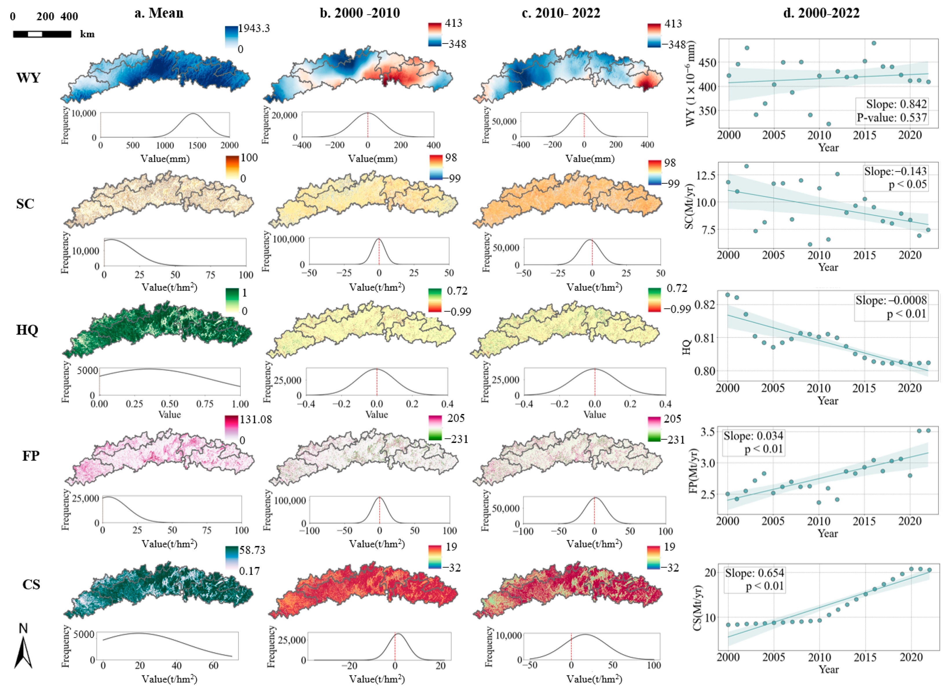
Over the past 23 years, the ESs have exhibited significant fluctuations, with their spatial distribution showing marked heterogeneity. FP (slope = 0.034,
p < 0.01) and CS (slope = 0.654,
p < 0.01) both demonstrated a highly significant increasing trend, while HQ showed a significant declining trend (slope = −0.0008,
p < 0.01). SC (slope = −0.143,
p = 0.537) also exhibited a significant decrease. Although WY (slope = 0.842,
p > 0.05) showed a slight upward trend, the change was not statistically significant (
Figure 2). The responses of different ecosystem services to environmental changes may differ significantly, likely due to various factors, including but not limited to external disturbances and the complexity of ecosystem responses. The spatial distribution patterns revealed that HQ and CS shared similar high-value areas located in the east and north. High-value SC areas were concentrated near the Nanling Mountains. The high-value areas of FP were found in the central and western parts, and the rest of the regions were evenly distributed. WY exhibited a spatial distribution with higher values in the central and eastern parts and lower values in the western parts, likely due to variations in the terrain altitude. The western plateau mountains have less precipitation and higher surface runoff.
From 2000 to 2010, the total WY in the study area changed slightly, with large spatial differences: a marked increase occurred in the east, and decrease occurred in the central part. After 2010, the decline shifted westward, resulting in reduced increases and only minor gains along the eastern edge. WY declined overall during this period. From 2000 to 2010, SC increased in the Nanling region; however, subsequent years saw significant changes across the entire area, ultimately leading to an overall decline. The HQ values were generally high throughout the region, with an overall distribution predominantly exceeding 0.7. There was a slight decrease from 2000 to 2010, followed by minimal changes thereafter. FP was mainly concentrated in flatter areas surrounding urban regions and exhibited a dispersed distribution. High CS values were mainly distributed in mountainous areas, which is related to the distribution of forests. The increase in CS from 2000 to 2010, followed by a more pronounced increase, is possibly linked to China’s ecological protection policies and initiatives, such as afforestation.
3.2. Interactions Among ESs at Different Scales
3.2.1. Spatial Distribution of Trade-Offs and Synergies
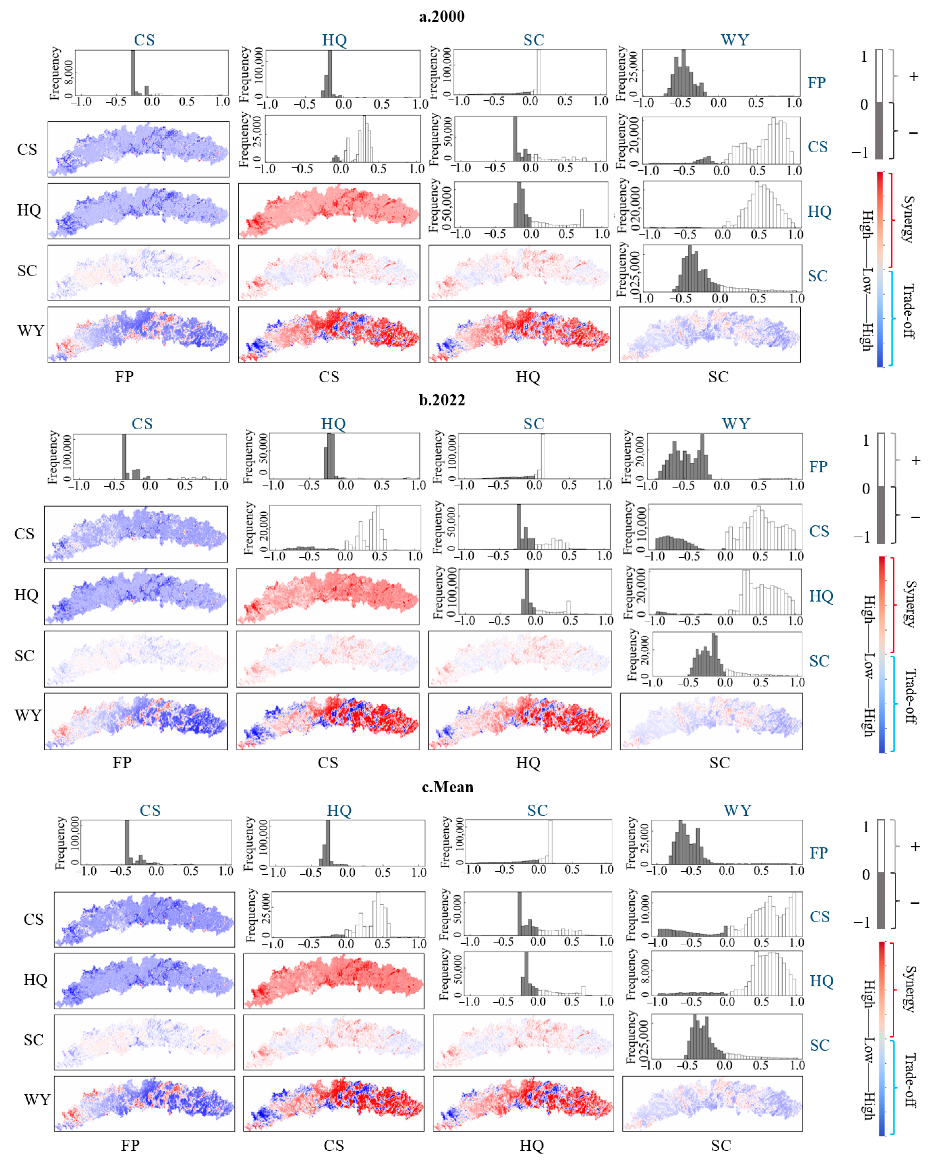
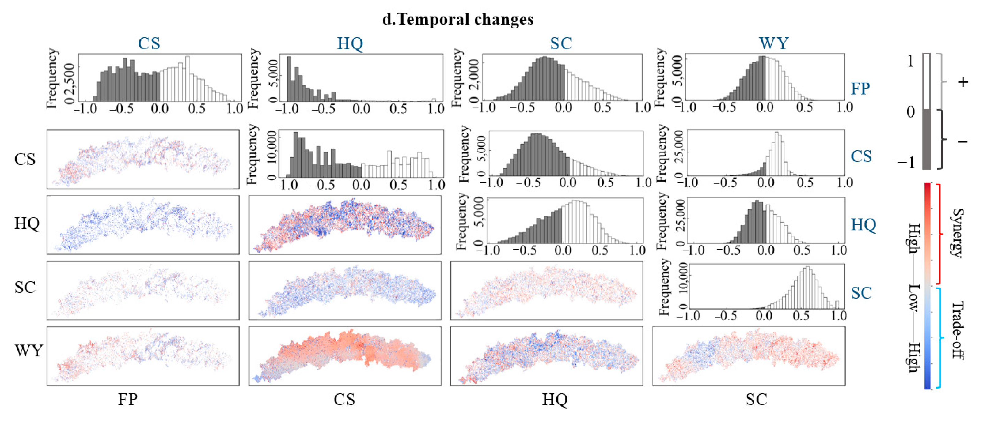
From a spatial distribution perspective, trade-offs and synergies among the ESs exhibited minimal variation over the years, with distinct correlations observed in the temporal dynamics of specific ESs (
Figure 3). Notably, trade-offs predominated in the FP–CS, FP–HQ, FP–WY, CS–SC, HQ–SC, and SC–WY relationships, while spatial synergies were primarily evident in the FP–SC, CS–HQ, CS–WY, and HQ–WY relationships. The regions with strong trade-offs in the FP–CS, FP–HQ, FP–SC, FP–WY, CS–WY, HQ–WY, and SC–WY relationships were concentrated in the western Yunnan–Guizhou Plateau and the Nanling Mountain Range, characterized by higher altitudes. The CS–HQ, CS–WY, and HQ–WY relationships demonstrated significant strong synergies. Among them, the CS–HQ trade-off was distributed throughout the entire region, and the strong trade-offs of CS–WY and HQ–WY were localized primarily in the central and eastern regions. From the temporal perspective, trade-offs and synergies involving CS–HQ, CS–WY, HQ–WY, and SC–WY exhibited more pronounced relationships compared to the others (
Figure 3d). CS–HQ and HQ–WY had more spatial trade-off relationships, while the CS–WY and SC–WY relationships primarily exhibited synergies.
3.2.2. Overall Characteristics of Trade-Offs and Synergies
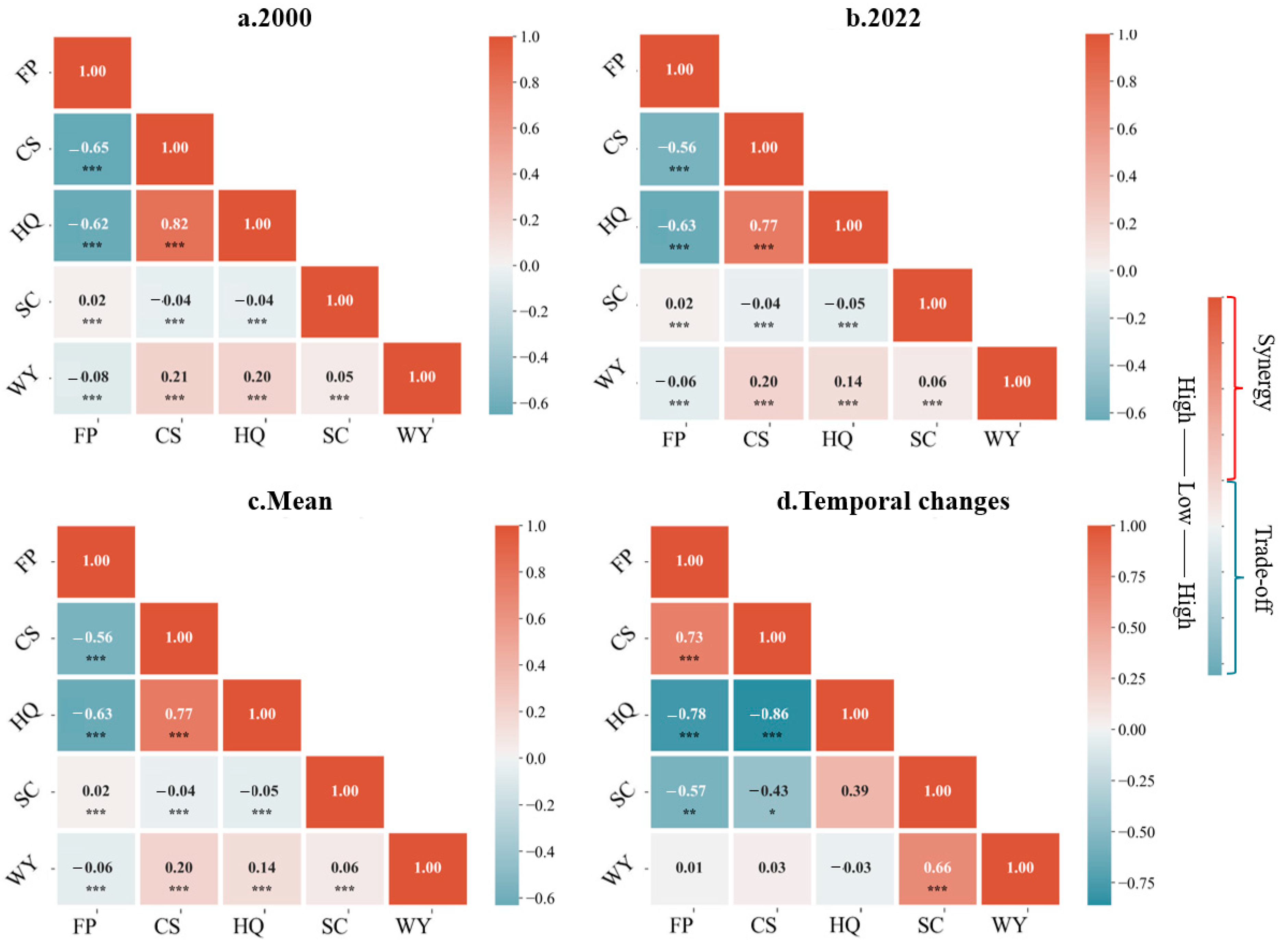
Regarding the overall characteristics, the correlations among the ESs from 2000 to 2022 remained consistent, with all results showing significant correlations (
p < 0.001) (
Figure 4). Positive correlations included the FP–SC, CS–HQ, CS–WY, HQ–WY, and SC–WY relationships. Conversely, negative correlations included the FP–CS, FP–HQ, FP–WY, CS–SC, and HQ–SC relationships.
Figure 4c shows the average correlation strength between the indicators in the past 23 years, which aligns closely with that of individual years. There were strong negative correlations among the FP–CS (r = −0.56) and FP–HQ (r = −0.63) relationships. These negative relationships arose because FP often necessitates land clearing and intensive agriculture, which can reduce vegetation cover and CS. Additionally, agricultural expansion frequently leads to the destruction of natural habitats, resulting in reduced biodiversity and HQ. By contrast, the CS–HQ relationship (r = 0.77) showed a strong positive correlation.
Figure 4d illustrates the correlations among the ESs over the 23-year period, where the FP–CS, FP–HQ, FP–SC, CS–HQ, CS–SC, and SC–WY relationships exhibited significant correlation characteristics (
p < 0.001). FP exhibited a significant negative correlation with HQ and SC, with correlation coefficients of −0.78 and −0.57, respectively. This is attributed to FP activities often requiring extensive land area, which typically involves alterations to the land and environment, consequently compromising HQ and SC. Similarly, CS also exhibited a significant negative correlation with HQ and SC, with correlation coefficients of −0.86 and −0.43, respectively. The correlations between FP and CS and between SC and WY were both highly significant, at 0.73 and 0.66, respectively. The correlation between FP and CS is attributed to increases in carbon emissions and decreases in carbon sinks resulting from land use changes and agricultural management practices, whereas the SC–WY relationship is due to the crucial role of vegetation cover and healthy soil structure in reducing erosion and increasing water infiltration.
3.3. Ecosystem Service Bundles
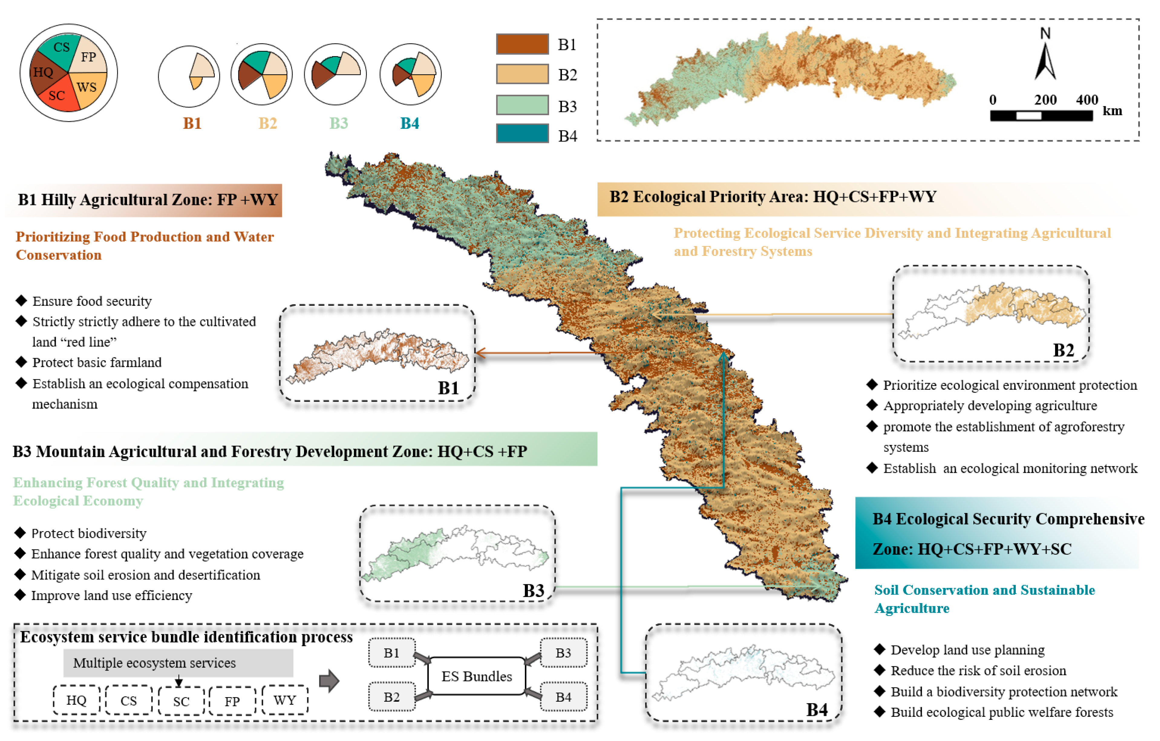
The SOM analysis identified four distinct ES bundles within the SHMB (
Figure 5). Bundle 1 (B1, hilly agricultural zone) includes FP and WY. This bundle is uniformly distributed across the study area, accounting for 21.29% of the total area. Bundle 2 (B2, ecological priority zone) encompasses HQ, CS, FP, and WY and is primarily concentrated in the central and eastern regions of the study area, covering 45.70% of the area. Bundle 3 (B3, mountainous agricultural and forestry development zone) contains HQ, CS, and FP and is mainly distributed in the western part of the study area, with a small amount distributed in the eastern part, accounting for 31.43% of the total area. Bundle 4 (B4, comprehensive ecological security zone) includes HQ, CS, FP, WY, and SC. This bundle is primarily located in the central region of the study area and has the smallest proportion, at 1.58%. These bundles highlight the spatial heterogeneity and varying priorities of the ESs in the SHMB, providing essential insights for targeted ecological management and regional planning.
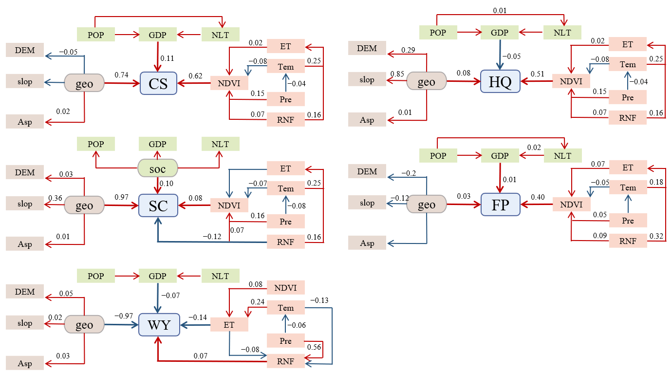
3.4. Drivers of ESs
CS is primarily affected by geography and vegetation, with path coefficients r of 0.74 and 0.62, respectively. By contrast, socioeconomic factors exert a minor impact, with a coefficient of only of 0.11. Additionally, while temperature promotes evapotranspiration, this process is counteracted by increased precipitation. Although DEM, slope, and aspect do not have significant impacts on CS alone, their combined effects are crucial for promoting vegetation growth, which in turn influences CS. Socioeconomic factors exert a minimal impact on CS across the region. The primary pathway for this influence is through population growth and urbanization, which stimulate GDP growth. GDP serves as a more effective indicator of socioeconomic factors, thereby reflecting the associated increase in CS.
The most important factor affecting HQ change is vegetation, with a path coefficient r of 0.51. The NDVI reflects the vegetation conditions and is closely related to precipitation and temperature. Increased precipitation enhances vegetation growth by providing additional water supply, while elevated temperatures may increase evaporation, resulting in water loss that negatively impacts vegetation growth. Geographical and social factors have relatively minor impacts on HQ. Among the geographical factors, there is a positive correlation with HQ (r = 0.08), with slope showing the highest impact on HQ (r = 0.85). Population density and the nighttime light index indirectly affect habitat quality through their influence on GDP levels. Specifically, higher GDP levels are generally associated with lower HQ (r = −0.05), suggesting that economic development may be accompanied by a certain degree of ecological environmental pressure.
For SC, geographic factors play a crucial facilitating role, exhibiting a substantial positive influence, with a path coefficient of r = 0.97. Among the geographical factors, slope has the greatest influence on SC, with a correlation coefficient of r = 0.36, while the effects of DEM and aspect are relatively minor. Social and economic factors have a small positive effect on SC, with a coefficient of r = 0.1, primarily due to the combined influence of multiple factors. Environmental factors influence SC changes, particularly increased runoff, negatively affecting SC, with impacts further mediated through evapotranspiration and vegetation dynamics. Increased vegetation promotes SC, with a coefficient r of 0.08, which stems from the soil-fixing ability of vegetation roots.
FP serves as a vital source of sustenance for human life. The relationship between the NDVI and FP is significant, with a path coefficient of r = 0.4, indicating that increases in the NDVI correspond to higher grain yields. Essential factors, such as increased precipitation, evapotranspiration, and runoff, ensure sufficient water supply and circulation for crops. Although individual topographic factors, such as elevation, slope, and aspect, have a negative impact on geographical factors, when considered together (r = 0.04), they can mildly promote FP through various mechanisms. Meanwhile, population density and the nighttime light index indirectly exert a positive influence on FP by affecting GDP levels (r = 0.01).
Among the factors affecting WY, elevated evaporation is detrimental to water conservation, while runoff contributes positively. The interplay among temperature, precipitation, and vegetation further complicates their effects on evaporation and runoff. Both geographic and socioeconomic factors exhibit negative effects on WY. The primary influence comes from topographic factors, which show a strong negative correlation, with a coefficient of −0.97. DEM, slope, and aspect all have significant impacts on topographic factors, with comparable effects. Socioeconomic factors exert a relatively small negative influence on WY (r = −0.07). Population density and the nighttime light index positively affect GDP by reflecting the intensity of economic activities, and the growth of GDP, in turn, negatively influences water yield (
Figure 6).
4. Discussion
This study advances traditional research on regional ESs by expanding its scope and application. First, we focused on the ESs in the SHMB, a vital ecological barrier in China. Due to its vast expanse, this region plays a significant role in biodiversity and ecological stability, making it essential to evaluate its ESs. Second, this study employed a long-term continuous sequence analysis, deepening our understanding of ESs and reflecting ecological processes more effectively than short-term or episodic studies. Previous studies have focused on ESs at the same spatial scale across different time points, at multiple spatial scales for a single time point, or across multiple spatial scales and time points. By contrast, our study, by combining pixel-level spatial distribution analysis and overall characteristic analysis with continuous long-term time series, offers a more comprehensive reflection of fluctuations and long-term trends. Furthermore, we integrated vegetation, geographical factors, socioeconomic factors, and climate factors and used the SEM framework model with prior knowledge to analyze the driving factors of the different ESs. To further refine this understanding, we employed the SOM approach to classify specific combinations of the ESs, clarifying the ecological functional layout of supporting, regulating, provisioning, and integrated services within the region. Overall, our comprehensive analysis enhances the understanding of ESs and their contributions to human well-being, thereby promoting rational ecological planning, governance, and sustainable development.
4.1. Spatiotemporal Dynamics of ESs
This study analyzed the spatiotemporal dynamics of the ESs over a continuous 23-year period. The analysis revealed that SC and HQ exhibited downward trends over time in the SHMB, while WY, FP, and CS showed overall upward trends. WY and SC displayed significant interannual variations, with pronounced fluctuations. The HQ values exhibited a slight decline, likely due to urbanization and land use change. The conversion of forest, grassland, and arable land to impervious surfaces threatens habitats, resulting in a decline in HQ [
35]. Spatially, HQ and CS exhibited similar patterns, with high-value areas in the eastern and northern regions, where forests provide habitats and enhance CS. Generally, regions with high forest cover and extensive grassland distribution also exhibit higher levels of CS [
36]. The extensive forest ecosystems in the region, combined with a favorable climatic environment, provide a conducive habitat for biodiversity. Additionally, these conditions facilitate CS [
35]. The high-value areas of SC and FP were mostly in the areas with dense vegetation cover and continuous cultivated land, and the retention effect of dense forest vegetation on precipitation effectively alleviates soil erosion. SC is also closely related to topographic factors. The areas with low SC values included karst rocky desertification regions and certain mountainous areas, which exhibit low soil conservation capacity due to factors such as concentrated precipitation, low vegetation cover, and human activities [
37]. FP generally increased but dipped in 2005 and 2010 due to natural disasters affecting agriculture, such as floods and heavy rains in Guangxi and other southern regions of China. Since 2010, the Natural Forest Protection Project and the Grain-for-Green Program have boosted CS. The spatial distribution of WY closely resembled that of precipitation. The high-value areas of WY were primarily attributed to higher precipitation, which provides more water to flow into surface runoff or percolate underground as groundwater, thereby increasing water yield. Additionally, WY is also influenced by vegetation. In general, vegetation helps to mitigate surface runoff and enhances groundwater recharge. Through the root channels of vegetation, water can more easily percolate into the soil, replenishing the groundwater supply [
38].
The spatial changes in the ESs across different stages are also noteworthy. From 2000 to 2010, the primary changes in WY occurred in northern Guangdong and southeastern Guizhou. This can be attributed to variations in precipitation over the years, including changes in the frequency and intensity of extreme weather events, which directly impacted runoff formation [
39]. With the implementation of the Forest Quality Improvement Project and Drinking Water Source Protection Project from 2010 to 2022, WY in Guangdong has been greatly improved. SC exhibited less variation during 2000–2010 but more pronounced changes from 2010 to 2022. This shift may be attributed to ecological protection policies implemented in China over the past few decades, such as reforestation and converting farmland to grassland, which have facilitated vegetation recovery and subsequently enhanced SC [
40]. HQ changed little in the two stages, but the overall ecological environment quality declined, which is related to the impact of urban construction on regional ecology [
41]. FP showed an upward trend over the past 23 years, indicating that the implementation of policies such as reforestation and farmland protection in the SHMB has been effective during this period [
42].
4.2. Trade-Offs and Synergies in ESs
Trade-offs and synergies in ESs show significant differences across service types [
43]. Many studies have demonstrated common trade-off relationships between FP and other ESs [
44]. As a provisioning service, FP contributes to agricultural productivity. However, agricultural ecosystems often conflict with biodiversity conservation, as they are less suitable for various plant and animal species. Moreover, agricultural ecosystems are less effective for carbon storage compared to forests and grasslands [
45]. Similarly, in our study, analysis of the overall temporal changes over the past 23 years indicated that FP and CS exhibit significant trade-off relationships with SC and HQ. This reflects the long-term impact of FP on ecological quality and the adverse consequences of vegetation degradation (
Figure 4d). Nevertheless, within the long-term sequence, only the pairs WY–SC and FP–CS exhibited significant synergies, a phenomenon closely related to the improvement in the quality of arable and forest land.
Based on our analysis of spatial distribution, strong trade-off relationships in ES correlated pairs (FP–CS, FP–HQ, FP–SC, FP–WY, CS–WY, HQ–WY, and SC–WY) were particularly evident in the high-altitude regions, such as the western Yunnan–Guizhou Plateau and the Nanling Mountains. The complex geographical and climatic conditions and diverse land use patterns in these regions lead to complex interactions among the ESs, which are profoundly influenced by socioeconomic factors. The combined effects of these factors make it increasingly challenging to achieve balance among FP, WY, HQ, and other ESs in these regions [
46]. The trade-off relationships between FP with CS and HQ were widely distributed across the study area. Notably, strong trade-offs were primarily concentrated in Honghe County of Yunnan and the central plains of Guangxi, which serve as major agricultural production regions, where the capacity for other ESs is relatively low [
47]. By contrast, the pairs of ESs related to CS and HQ (CS–HQ, CS–WY, and HQ–WY) exhibited significant synergies. Specifically, the synergy between CS and HQ was evident throughout the entire region, while strong synergies between CS and WY and between HQ and WY were primarily concentrated in the central and eastern regions. This phenomenon is closely related to the over 75% forest coverage in the study area, where vegetation cover typically exerts a positive impact on the ecological environment.
Trade-offs and synergies among ESs exhibit certain similarities, particularly in terms of the intensity of local service provision and spatial distribution, where both often display comparable patterns [
48]. In our study, a strong trade-off relationship appeared between HQ and CS, and strong synergistic relationships between CS and FP and between HQ and FP were consistent at different scales. This suggests that, in terms of spatial distribution, various ecosystem services are closely interconnected between adjacent pixels, and spatial aggregation patterns influence the overall service landscape at larger regional scales. Regarding the overall characteristics, significant shifts in the trade-offs and synergies among the ecosystem services were observed. These shifts reflect the dynamic changes in the competitive and complementary relationships among different services. Such changes may indicate adjustments in the relative demands of these services in response to alterations in land use or ecological conditions. This finding is consistent with the work of several scholars [
44,
49]. Therefore, this analysis provides crucial scientific evidence for understanding ecosystem services in the context of sustainable management and contributes to the further optimization of service provision.
Based on the results of the trade-off and synergy analysis, we found that although trade-off relationships are generally present, the synergy between certain services can be enhanced by improving land quality. Furthermore, the distribution of trade-offs and synergies is influenced by a combination of factors. Therefore, in managing and optimizing ESs, the interplay among geographical, climatic, and socioeconomic factors should be considered to promote the coordinated development of services.
4.3. Impact of Different Drivers on ESs
This study provides a comprehensive analysis of the impact of driving factors on the ESs in the SHMB. The spatial distribution of the ESs in the SHMB exhibited significant spatial heterogeneity, which stems from the multiple effects of socioeconomic, ecological and natural conditions [
50]. The spatial and temporal distribution of the ESs varied under different drivers, which were categorized into climatic factors, vegetation factors, geographic factors, and socioeconomic factors.
- (1)
Combined effects of climate and vegetation factors
Precipitation, as the primary water source for plant growth, is generally positively correlated with vegetation growth [
51,
52]. Adequate rainfall promotes plant growth, thereby increasing regional CS, improving soil quality, and enhancing food production capacity [
53]. Vegetation factors, through processes such as photosynthesis and organic matter accumulation, increase CS and FP capacity. Additionally, they help to slow down runoff, retain soil, and filter pollutants, thereby improving water quality and soil health [
54].
- (2)
Geographic factors
Geographic factors significantly influence ESs through hydrological processes, vegetation distribution, and geographic features [
55]. In the SHMB, topography positively impacts factors such as CS and SC. The rich vegetation in the plateaus and mountainous areas promotes plant growth and organic matter accumulation, thereby enhancing carbon storage. Furthermore, SC is closely related to elevation, slope, and aspect. High-altitude and steep areas are often more susceptible to soil erosion due to substantial variations in runoff. In karst rocky desertification areas, although the groundwater system is well developed, the soil layer is thin and prone to erosion, resulting in low vegetation coverage. This leads to a significant negative correlation between WY and topographical factors [
56].
- (3)
Dynamic impact of socioeconomic factors
Human activities and policy interventions often exert complex and dynamic effects on ESs through socioeconomic factors. Although the overall impact of these factors on the ESs in the SHMB is relatively low, their influence should not be underestimated. In certain areas, limitations due to natural conditions, insufficient policy support, and fragile ecological environments prevent socioeconomic factors from having a noticeable impact. Nevertheless, with the backing of ecological protection policies, rational land use and management strategies can still optimize the configuration of ESs in localized regions.
In summary, climate, vegetation, geography, and socioeconomic factors collectively influence the distribution and changes of ESs through complex interactions. This multi-layered spatial heterogeneity provides a scientific basis for the management and optimization of ESs in the region. Understanding the mechanisms of these factors will assist in formulating more effective ecological management policies to address ecological demands at different scales. At the same time, threshold effects of influencing factors also exist within the ecosystem. For instance, the threshold effects of temperature and precipitation on ecosystems, crop yields, and water resource management require further investigation.
4.4. Insights from ES Bundles for ES Management
Rational land management and utilization strategies are crucial for enhancing the supply of ESs. Based on the characteristics of the ESs, the study area was divided into four functional types to enhance the efficiency of the integrated management of multiple ESs in the SHMB. By analyzing the structural composition, interactions, and driving factors of various bundles, adaptive ecological management measures can be proposed (
Figure 5):
B1—Hilly Agricultural Zone: Prioritizing Food Production and Water Conservation.
The main function characteristics of region B1 are FP and WY, highlighting the importance of farmland protection and water resource management. To ensure food security, it is essential to strictly adhere to the cultivated land “red line,” particularly by protecting basic farmland [
57]. In addition, establishing an ecological compensation mechanism to provide reasonable compensation to the providers of ESs in benefiting areas can effectively incentivize farmers and local governments. This approach will further enhance farmland environments and FP, promoting a positive interaction between food production and the ecological environment in the region.
B2—Ecological Priority Area: Protecting Ecological Function Diversity and Integrating Agricultural and Forestry Systems.
Region B2 encompasses HQ, CS, FP, and WY and is located in the Nanling Mountain Range area of the watershed between the Yangtze and Pearl River Basins. The management strategy for this area should prioritize ecological environment protection while appropriately developing agriculture, thus achieving a balance between ecological priorities and agricultural development. It is recommended to promote the establishment of agroforestry systems to enhance the region’s ecological resilience. Building on this, an ecological monitoring network should be established and improved to regularly assess the environmental quality of the watershed. This will facilitate the early detection and response to changes in ecosystem health, thereby ensuring the ecological stability of the watershed.
B3—Mountain Agricultural and Forestry Development Zone: Enhancing Forest Quality and Integrating Ecological Economy.
B3 encompasses the karst landforms in southwest China, with the key ESs including HQ, CS, and FP. Due to its topographical and soil characteristics, this area faces significant challenges related to soil erosion and land degradation. Rational ecological management strategies should integrate agricultural and forestry economic development to enhance forest quality and vegetation coverage. This will help to maintain carbon balance, conserve soil and water resources, purify the air, and protect biodiversity. Concurrently, the region needs to implement comprehensive management measures to mitigate soil erosion and desertification, thereby improving land use efficiency and achieving the sustainable development of agricultural and forestry resources.
B4—Ecological Security Comprehensive Zone: Soil Conservation and Sustainable Agriculture
B4 serves as an integrated ecological security region, encompassing HQ, CS, FP, WY, and SC. Although it occupies a relatively small proportion of the study area, this region has high ecological value. SC should be prioritized in agricultural development, and agricultural land should be allocated appropriately [
36]. Land use planning should be developed based on factors such as topography, soil type, and climatic conditions, avoiding cultivation in areas unsuitable for farming to reduce the risk of soil erosion.
In summary, through rational functional zoning and targeted ecological management strategies, the supply efficiency of different types of ESs will be significantly improved. Collaborative management among different functional areas can not only optimize the benefits of individual functions but also achieve a balanced supply of ESs through integrated measures, providing a scientific basis for regional ecological security and sustainable development in the SHMB.
5. Conclusions
ESs are crucial for maintaining ecological balance and supporting human existence. A comprehensive understanding of their spatiotemporal variation and interactions is essential for formulating effective ecological management strategies. This study focused on the typical ecological barrier zone in the hilly mountainous regions of southern China and systematically analyzed the spatiotemporal variations in five major ESs: food production (FP), carbon storage (CS), water yield (WY), habitat quality (HQ), and soil conservation (SC). Through analysis of trade-offs and synergies, the interaction relationships among the ESs were clearly identified, along with the key driving factors and clustering characteristics underlying their changes.
The research results indicated that, over the past 23 years, the ESs exhibited significant fluctuations and their spatial distribution showed notable heterogeneity. This finding suggests that long-term sequence analysis more effectively captures the dynamic changes in ecological processes, underscoring the limitations of short-term and periodic studies. Additionally, the analysis of trade-offs and synergies allows for a more comprehensive understanding of the interactions among ESs. The results also demonstrated significant scale effects, with spatial integration becoming more pronounced from the micro to regional scales, while temporal variations reflected the dynamic changes in the competitive and complementary relationships among different services concerning resource allocation.
This study further explored the multiple drivers that influence changes in ESs, including geographic, socioeconomic, vegetation, and climatic factors. The combined effects of these factors impact the temporal and spatial variations of ESs, providing important evidence for regional ecological management. Additionally, this study identified the predominant combinations of ESs in different regions through bundle analysis, offering practical strategies for optimizing ecological management and conservation measures.
In summary, this study not only deepens the understanding of ESs but also highlights the importance of the relationships between them. Our analysis provides a better reflection of the fluctuations and long-term trends of ESs and offers scientific support for policymakers, thereby facilitating the effective implementation of ecological management.


 ,
, 
