Investigation of Spatio-Temporal Simulation of Mining Subsidence and Its Determinants Utilizing the RF-CA Model

Abstract

It is important to carry out timely scientific assessments of surface subsidence in coal resource cities for ecological environmental protection. Traditional subsidence simulation methods cannot quantitatively describe the driving factors that contribute to or ignore the dynamic connections of subsidence across time and space. Thus, a novel spatio-temporal subsidence simulation model is proposed that couples random forest (RF) and cellular automaton (CA) models, which are used to quantify the contributions of driving factors and simulate the spatio-temporal dynamic changes in subsidence. The RF algorithm is first utilized to clarify the contributions of the driving factors to subsidence and to formulate transformation rules for simulation. Then, a spatio-temporal simulation of subsidence is accomplished by combining it with the CA model. Finally, the method is validated based on the Yongcheng coalfield. The results show that the depth–thickness ratio (0.242), distance to the working face (0.159), distance to buildings (0.150), and lithology (0.147) play main roles in the development of subsidence. Meanwhile, the model can effectively simulate the spatio-temporal changes in mining subsidence. The simulation results were evaluated using 2021 subsidence data as the basis data; the simulation’s overall accuracy (OA) was 0.83, and the Kappa coefficient (KC) was 0.71. This method can obtain a more realistic representation of the spatio-temporal distribution of subsidence while considering the driving factors, which provides technological support for land-use planning and ecological and environmental protection in coal resource cities.

1. Introduction

With the rapid development of the modernization of coal resource cities, the main position of coal as an energy source will not change for some time [1,2,3]. While the exploitation of coal resources promotes social development and economic growth, it also has significant impacts on the regional ecological environment, the most prominent manifestation of which is surface subsidence and its disturbance of the ecological environment [4,5,6,7]. To achieve the sustainable development of coal resource cities and decrease the losses caused by mining subsidence, it is essential to clarify the driving factors affecting subsidence, establish a spatial and temporal simulation model that identifies subsidence in coal mining, and obtain the most “realistic” evolution of ground subsidence as much as possible, so as to provide technical support for urban planning and ecological and environmental protection.

The most commonly used surface subsidence acquisition methods mainly include numerical simulations of mining subsidence and the subsidence inversion method based on time-series interferometric synthetic aperture radar (InSAR) technology. Litwiniszyn et al. [8] constructed a stochastic medium model based on the probabilistic integral method to predict the spatial distribution of surface subsidence. M.I. Álvarez-Fernández et al. [9] and C. González-Nicieza et al. [10] presented a novel approach for predicting surface subsidence by combining the Knothe theoretical model with consideration given to the time factor, completing the analysis of spatial variations in subsidence. Behrooz et al. [11] proposed a numerical simulation method based on finite elements to set simulation parameters in combination with the reality of the mining and geological situation of a mining area to predict the spatial distribution of mining subsidence. Alam et al. [12] integrated factors such as the surface, mining plate, fault, and embankment and used the displacement discontinuity method to simulate subsidence and future subsidence distributions. Jeon et al. [13] proposed a new approach that combined numerical simulation and statistical analyses for predicting the spatial distribution of coal mining subsidence based on FLAC 2D 7.0 simulation software. Existing numerical simulation methods require the determination of too many parameters, leading to subjectivity and uncertainty in the simulation results.

With the development of remote sensing technology, scholars have used the InSAR technique to quickly obtain surface subsidence spatial distribution data, which can be simply processed and are widely used in surface subsidence extraction [14]. Ferretti et al. [15] proposed permanent scatterer interferometry technology for the measurement of surface subsidence, an approach that has been applied successfully in the Ancona area. Milczarek et al. utilized the PS-InSAR technique in combination with Envisat ASAR data for surface subsidence surveying in the former Wałbrzych coalfield [16]. Zhang et al. [17] combined Sentienl-1A data with PS-InSAR and DS-InSAR technology to monitor the surface subsidence of the Hancheng coal mine. Yang et al. [18] processed Sentinel-1A data using SBAS-InSAR to conduct a subsidence monitoring study of a mine site in Wuan. Wang et al. [19] utilized DS-InSAR technology and fifty-five Sentinel-1A radar images for surface subsidence monitoring in the Yuncheng coal mine. The essence of using the InSAR technique to acquire data on spatio-temporal changes in subsidence is to obtain the spatial distribution of subsidence of each time-series image by analyzing time-series surface subsidence data pixel-by-pixel.

Influenced by a variety of factors such as complex geological conditions, surface topography, and mining conditions, the formation mechanism of subsidence in coal mines is complicated, and it is difficult to obtain the estimated spatio-temporal evolution of surface subsidence using traditional technical means and prediction models. At the same time, mining areas are ecologically sensitive, and the ecological disturbances caused by coal mining are far-reaching and irreversible [4,20]. Existing simulation models do not comprehensively consider the driving factors of subsidence, thus failing to clarify the degree of contribution of these factors to subsidence. Therefore, taking into account and quantifying the degree of contribution of subsidence-driving factors when building a spatio-temporal subsidence simulation model is necessary for the formulation of the simulation model transformation rules. With the rapid development of modern computer technology, some machine learning models are beginning to be introduced into the formulation of transformation rules and the acquisition of relevant parameters in the study of the spatio-temporal evolution of features [21,22,23,24]. Among them, the more commonly used random forest (RF) algorithm can avoid the influence of the subjective selection of the driving factors and can better deal with nonlinear problems [25,26,27,28,29]. At the same time, the algorithm can quantitatively describe how much the driving factors contribute to the model.

In addition, several studies modeled time and space separately, ignoring the dynamic connections between subsidence and time and space. To address this, Wang et al. [30] proposed a spatio-temporal prediction model for surface subsidence based on CEEMDAN-CNN-BiLSTM. Liu et al. [31] extracted the spatio-temporal features of tunnel vault subsidence and accomplished the prediction of subsidence by combining the CNN, TCN, and the attention mechanism model. Related studies have shown that deep learning algorithms are highly dependent on the quality and quantity of training samples when training models. When the number of samples is small, the accuracy of the model decreases significantly [32,33]. The simulation of the spatio-temporal evolution of features based on the CA model solves the above problems effectively. This method breaks down complex mathematical modeling by treating the computational area as individual grids, setting key attributes for each grid, and then setting local and overall rules to establish connections between the grids, which enables simulations to be conducted with small samples. Yang et al. [34] applied the principle of the CA model to the simulation of the urbanization development of tourist-type towns and established a CA model to simulate the development of tourist towns from 2010 to 2015. Zhang et al. [35] simulated the spatial and temporal distribution of Guangdong Province’s urban land by utilizing the CA model to assess the role of future urban increases on carbon storage. Chen et al. [36] established a CA model for coal mining subsidence by combining the CA model and coal mining technology to simulate the coal mining subsidence process. Existing studies confirm the possibility that the CA model can be used to simulate mining subsidence. At present, the model is mainly used in the analysis of surface cover change and urban expansion, with fewer applications in mining subsidence analyses [37].

To address the problems raised by previous studies, a novel RF-CA subsidence simulation model is introduced in this study. The model first utilizes the RF algorithm to formulate the conversion rules of simulation and clarify the contribution of driving factors to subsidence. Then, the model is combined with the CA model to achieve a spatio-temporal dynamic subsidence simulation. This method can be adopted to quantify the driving factors of subsidence and determine the mechanism of subsidence and the change rule, offering technical support for supervision agencies in their formulation of subsidence protection strategies under different mining environments and providing a scientific basis for ecological and environmental protection.

2. Methods and Materials

2.1. Methods

The RF and CA models were coupled to simulate the spatio-temporal progression of mining subsidence in this study. Firstly, the surface subsidence data of the base year were obtained using SBAS-InSAR technology. Secondly, information on the subsidence evolution mechanism and the contributions made by the driving factors to subsidence was obtained based on the RF-CA model, and then a mining subsidence simulation was completed. Finally, the simulation accuracy of the model was evaluated, and the spatio-temporal progression features of mining subsidence were analyzed. A flow chart of this study is shown in Figure 1, and the research methodology is described in the following sections.

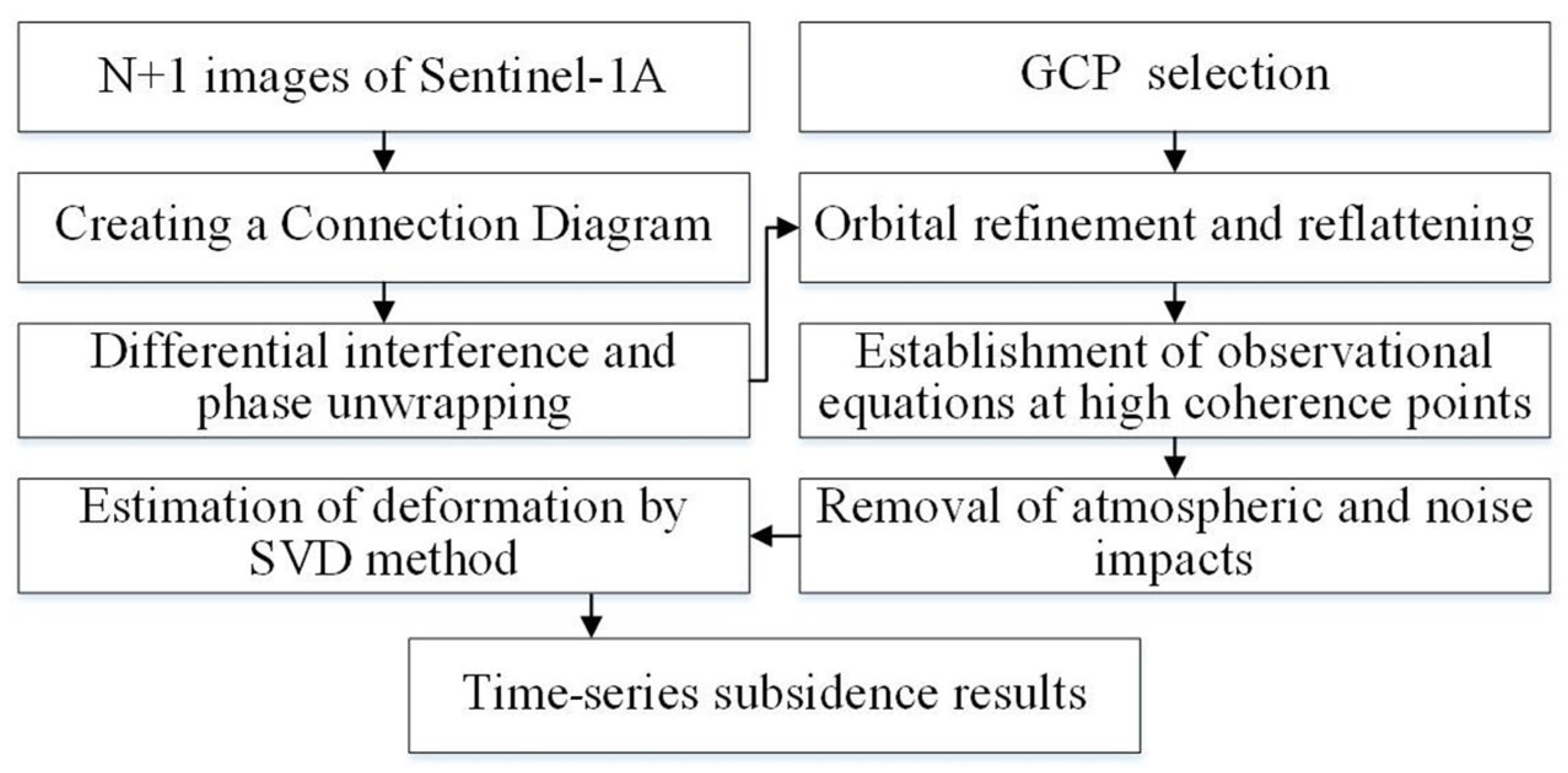
2.1.1. Subsidence Data Acquisition Based on InSAR Technology

Sentinel-1A data were manipulated using SBAS-InSAR technology to extract time-series subsidence data based on ENVI5.6 SARscape software [38]. The basic idea of the SBAS-InSAR technique is to efficiently inhibit the errors brought about by spatio-temporal incoherence and atmosphere delay. The SBAS-InSAR technique divides the acquired SAR images into several combinations of narrow baseline datasets and sets reasonable temporal and spatial thresholds to obtain interferograms with good coherence. The interference pattern within the narrow baseline grouping is then subjected to differential interferometry, filtering, and phase untangling. Time-series subsidence was calculated using the singular value decomposition (SVD) method [39], and the base mining subsidence data for 2019, 2020, and 2021 were obtained for simulation. This method is applicable for the extraction of mining subsidence data for natural circumstances [40,41,42], and the data processing procedure is illustrated in Figure 2.

With a view to matching the needs of the model input, the surface subsidence maps for each period were reclassified and processed based on ArcGIS 10.7 software. The surface subsidence data were categorized into five types: no subsidence (subsidence ≥ 0 mm), slight subsidence (−10 mm ≤ subsidence < 0 mm), moderate subsidence (−20 mm ≤ subsidence < −10 mm), more serious subsidence (−40 mm ≤ subsidence < −20 mm), and serious subsidence (subsidence < −40 mm). Three classified images of the subsidence distribution are shown in Figure 3.

2.1.2. Driving Factor Correlation Analysis Methods

An attempt was made to avoid problems such as redundant information between the selected driving factors, which results in the model being unable to correctly judge real relationships between the driving factors and subsidence. Therefore, two indexes, the variance inflation factor ($VIF$) and the tolerance ($TOL$), were selected for testing multiple covariances of the subsidence-driving factors [43]. Meanwhile, this study also used the Pearson correlation coefficient (PCC) to carry out the correlation analysis of the subsidence-driving factors.

$VIF$ is the ratio of the variance in the presence of multicollinearity among the subsidence-driving factors to the variance in the absence of multicollinearity (Equation (1)), and $TOL$ is the inverse of $VIF$ (Equation (2)).

$$VIF={\displaystyle \frac{1}{1-R_i^2}}$$

(1)

$$TOL={\displaystyle \frac{1}{\mathit{VIF}}}$$

(2)

where $R_i^2$ is the correlation coefficient of the regression analysis of one of the subsidence-driving factors on the remaining driving factors. When $VIF<10$ or $TOL>0.1$, the level of covariance among the driving factors is low, and vice versa.

The linear correlation between the two variables was quantified using the PCC, which has a value between −1 and 1 (Equation (3)).

$$r={\displaystyle \frac{1}{n-1}}{\sum }_{i=1}^n\left({\displaystyle \frac{X_i-\overline{X}}{\sqrt{X_i-\overline{X}}}}\right)\left({\displaystyle \frac{Y_i-\overline{Y}}{\sqrt{Y_i-\overline{Y}}}}\right)$$

(3)

where $X_i,Y_i$ are the two driving factor values, respectively; $n$ is the number of driving factor samples; and $\overline{X}$, $\overline{Y}$ denote the average values of the respective driving factors. A strong relationship between the two driving factors can be recognized when $\left|r\right|>0.5$.

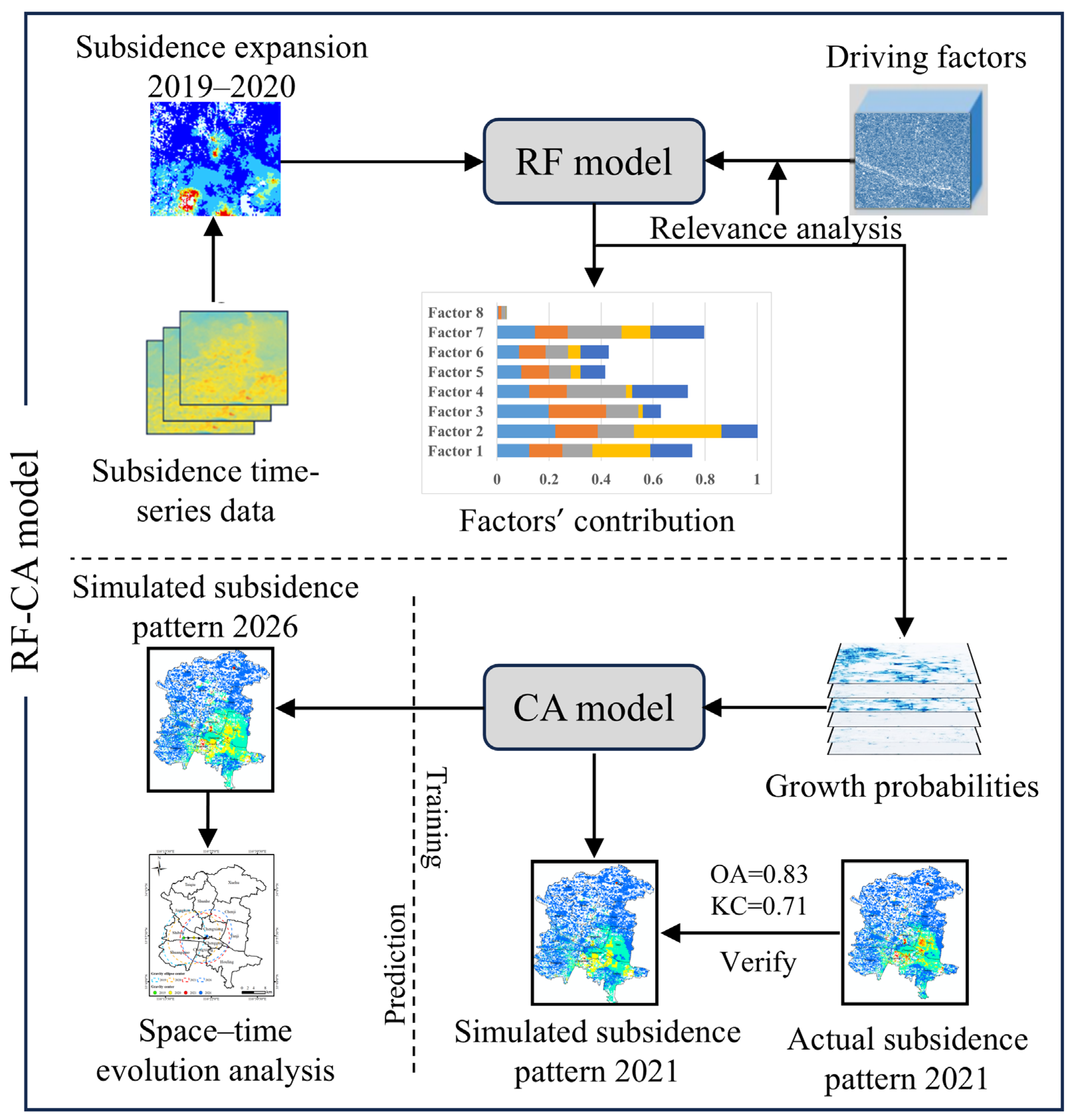
2.1.3. Simulation of Subsidence Evolution Based on RF-CA Model

The RF-CA model proposed in this research consists of two parts, including the RF model for determining the driving factors’ contribution and the probability of subsidence development and the CA model for simulation of the spatio-temporal evolution of mining subsidence.

(1)

Random forest (RF) model

The RF model is a machine learning model proposed by Breiman, which is effective when dealing with the problem of multicollinearity between variables [23,44], is less susceptible to overfitting, and is more resistant to abnormal values and noise [28,45]. It is generally recognized for its accuracy and sufficiently flexible mechanism, as well as its ability to handle small-sample feature spaces. Most notably, the RF model provides an interpretable measure of the contribution of the global variable for each variable [46]. Therefore, the algorithm was utilized to determine the transformation rules for subsidence. The RF algorithm was used to sample the portion of the $t_1$ moment to the $t_2$ moment where each type of subsidence type had changed. Then, the probability of subsidence development during this period was determined along with a quantitative explanation of the degree of contribution of different driving factors to subsidence development.

The core purpose of random forest in feature contribution assessment is to compare the mean value after summing the size of the contribution generated by each characteristic onto each tree of the random forest. The Gini index is normally used to measure the size of the contribution of each driving factor; the formula for calculating the Gini index is shown in Equation (4) [47,48,49].

$$Gini(s)=1-{\sum }_{i=1}^K{s}_i^2$$

(4)

where $i$ indicates the category, and $s_i$ indicates the corresponding category’s weight.

(2)

Cellular automata (CA) model

The CA model is the lattice dynamics model first proposed by von Neumann. In contrast to the traditional formula-based geography models, the CA model, as a discrete dynamics model with spatio-temporal characteristics, can not only simulate and analyze general complex systems but also has more advantages for geographically complex systems with spatio-temporal evolution characteristics [36]. It is a powerful tool for modeling a wide range of highly complex geographic phenomena such as ecology, the environment, and natural disasters. The model has its own unique advantages, such as its application in geographic phenomena with spatial self-organization, such as land-use dynamics, fire spread, and flooding [50].

The CA model includes cellular spaces and their states, transformation rules, and domains. The CA is essentially a model composed of cellular and action rules, which drive system changes through internal cellular interactions. The CA model can be described as follows:

$$S^{t+1}=f(S^t,N)$$

(5)

where $S$ is a finite set representing each cellular state, t denotes the time, $f$ denotes the inter-transformation rule between cells, and $N$ denotes the cellular neighborhood.

The sampling rate of the RF model is set to 0.01, and the number of RF training features is set to 8 in line with the number of driving factors; the domain range of the CA model is set to 3, the threshold of plaque generation is set to 0.5, and the probability of the random plaque seed is set to 0.0001; and the transformation rules follow the transfer probability in the Markov calculation result, with those set with a probability lower than 0.1 to 0.

2.1.4. Accuracy Evaluation

In this research, the accuracy of the model simulation results was assessed using overall accuracy (OA) and the Kappa coefficient (KC). OA is a commonly used index that compares the number of accurately predicted subsidence types in the results of a simulation with the total number of subsidence types and the expression shown in Equation (6). In addition to OA, the KC was used as an accuracy validation metric. The KC is able to overcome the problem of overreliance on the selected samples and utilizes a statistical approach to assess the correspondence between the simulated and measured images, with the expression shown in Equation (7) [51,52].

$$OA={\displaystyle \frac{\sum _{i=1}^k{m}_{ii}}{n}}$$

(6)

$$KC={\displaystyle \frac{m\sum _{i=1}^k{m}_{ii}-\sum _{i=1}^k{m}_{i+}{m}_{+i}}{m^2-\sum _{i=1}^k{m}_{i+}{m}_{+i}}}$$

(7)

where $n$ indicates the sum of samples; $k$ indicates the number of categories in the confusion matrix; $m_{ii}$ represents the number of correct predictions on row $i$ and column $i$ in the confusion matrix; and $m_{i+}$ and $m_{+i}$ represent the overall number of samples on row $i$ and column $i$, respectively. When the OA and KC values are larger, it indicates that the simulation result is better. When the KC value is in the range of 0.61 to 1.00, it indicates a high degree of coherence [53,54].

2.1.5. Analysis Methods for the Spatio-Temporal Evolution of Subsidence

(1)

Kernel density analysis method

To reveal the aggregation condition of mining subsidence more clearly, the space distribution of mining subsidence over time in the region was analyzed using the kernel density method; the expression is shown in Equation (8). Kernel density analysis associates each known point location and attribute value with the kernel function, determines the weight value according to the distance from the image element, sums the raster values, and displays the calculation results in layers with colors [55,56]. A higher kernel density value means that the distribution density of the subsidence area is higher and more clustered, and vice versa.

$$f_n={\displaystyle \frac{1}{nh}}\sum K\left[{\displaystyle \frac{{d(x,x}_i)}{h}}\right]$$

(8)

where $f_n$ is the estimate of the subsidence kernel density; $K$ is the kernel density function; $h$ is the bandwidth; $n$ is the number of subsidence point data in the bandwidth range; and ${d(x,x}_i)$ denotes the distance between the estimated point $x$ and the sample point $x_i$.

(2)

Center of gravity model

The planar center of gravity model is able to reflect the gravity center migration process of the subsidence area, and calculating the center of gravity position of the mining subsidence area in different periods can help in the analysis of the space transition processes of the subsidence area in two-dimensional space [34,57]. Equations (9) and (10) are as follows:

$$X={\displaystyle \frac{\sum _{i=1}^m{w_i\ast x}_i}{\sum _{i=1}^m{w}_i}}$$

(9)

$$Y={\displaystyle \frac{\sum _{i=1}^m{w_i\ast y}_i}{\sum _{i=1}^m{w}_i}}$$

(10)

where $X,Y$ are the mean coordinates of the center of gravity of the study object; $m$ is the number of subsidence units; $w_i$ is weighted by the subsidence area in different years; and $x_i$ and $y_i$ are the geometric coordinates of the center of gravity of the study object.

2.2. Materials

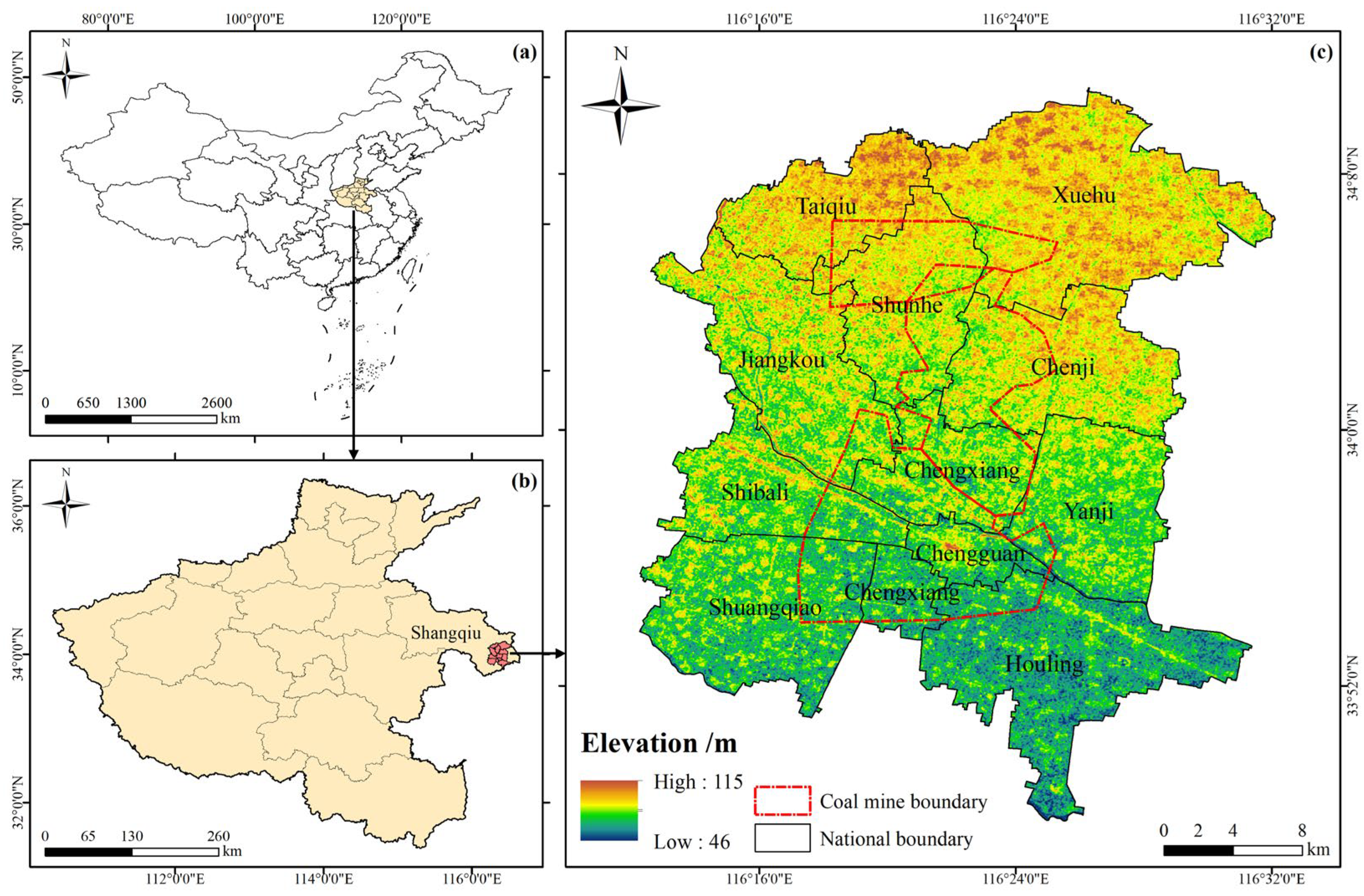
2.2.1. Overview of Study Area

The Yongcheng coalfield is situated in Shangqiu City in the southeastern region of Henan Province, China. It is a coal-rich area and is one of the six biggest smokeless coal bases in China, whose coal reserves account for 11.07 percent of the total reserved coal reserves in Henan Province. With its stable coal layers and easy mining environment, the coalfield is an essential coal manufacturing and backup area in East China, and its position in the coal industry is of strategic significance. The coalfield mainly includes a number of mines, such as Chensilou, Chengjiao, and Shunhe, and covers 12 townships, including Chengxiang, Chengguan, and Shunhe (Figure 4).

The Yongcheng coalfield has a flat terrain, and the surface of the region is dominated by arable land, which is one of the major grain-producing areas in Henan Province. It is evident that vigorous coal resource extraction will inevitably affect surface crops and human activity sites. Therefore, it is essential to clarify the spatio-temporal evolution of subsidence in the region.

2.2.2. Surface Subsidence Data

The SAR image data were acquired by the Sentinel-1A satellite. The SAR surface survey pattern is an interferometric broadband pattern with a width of 250 km, a C-band wavelength of 5.6 cm, VV polarization, a spatial resolution of 5×20 m, and a revisiting frequency of 12 d. The satellite has a high frequency of revisits, high coverage, and excellent timeliness and reliability [58]. In the data preprocessing stage, the influence of satellite orbital inaccuracy and topographic phases was removed by introducing orbit data and SRTM DEM data (30 m) (https://browser.dataspace.copernicus.eu/ (accessed on 10 January 2024)).

Due to the short coal mining cycle and the fact that subsidence occurs more quickly, in a bid to better study the mining subsidence law and avoid missing subsidence data due to temporal decorrelation, Sentinel-1A data with high spatio-temporal resolution were selected. Twenty-five images from Sentinel-1A covering the study area for the period 2019 to 2021 were selected for the experiment, and SBAS-InSAR technology was utilized for the preprocessing of the Sentinel-1A data. Previous researchers have already utilized survey-level data and GNSS supervision data to verify the dependability of the results extracted using this technology [59,60]. The extraction results were also in accordance with those of Xu et al., who used the same experimental program in this study area [41]. Finally, surface subsidence maps covering the Yongcheng coalfield in 2019, 2020, and 2021 were obtained. According to the geological report of the study area, the selected study period includes the initial, active, and recession stages of subsidence in different mining areas, and the selected study data are representative and can be used for model simulation.

In order to maintain consistency with the timing of the driver data, the subsidence area change information was extracted using the reclassified surface subsidence maps for 2019 and 2020 during the study period, and conversion rules were developed. In order for the validation data to cover as much of the mining cycle as possible, model simulation accuracy was verified using the reclassified surface subsidence map for 2021. To decrease the error pass-through uncertainty, the 2021 surface subsidence data were adopted as the preliminary year for model simulation inputs when predicting surface subsidence in 2026.

2.2.3. Subsidence-Driving Factor Data

When coal is mined, surface subsidence presents certain special patterns due to various factors such as geological conditions and surface environment. In this study, based on previous research results, eight driving factors were selected from two levels of mine geology and natural environment factors, as shown in

Table 1. Mining subsidence-driving factor data.

Types	Driving Factor Data	Data Source
Mining geological factors	Depth–thickness ratio	A coal mine in Henan Province, China
	Distance to working face
	Lithologic
Natural environmental factors	Distance to water	Landsat 8 image classification
	Distance to building
	Distance to railroad	Administrative division data
	Rainfall	National Tibetan Plateau Science Data Center
	Slope	Calculated from DEM (https://www.gscloud.cn/) (accessed on 15 January 2024)

. The mine geology factor is determined by the mining conditions of the coalfield itself, and when the nature of the overlying rock strata is certain, with the change in the depth–thickness ratio, the mine subsidence is centered on the working face and shows a certain regularity [61,62]. In addition, for the purpose of protecting surface safety and fully exploiting underground coal resources, coal mines have adopted the “three-under” mining technology, namely, mining underneath water bodies, buildings, and railroads [17,60]. Topography and rainfall also play a role in contributing to mine subsidence, so five natural environmental driving factors were selected for this study.

In an attempt to match the needs of model input, ArcGIS 10.7 software was used to rasterize each driving factor and unify the coordinate system. The rasterized map of each driving factor was multi-sampled at 30m resolution to keep the data format consistent.

3. Results

3.1. Correlation Analysis for Subsidence-Driving Factors

Two indicators, the variance inflation factor ($VIF$) and the tolerance ($TOL$), were selected to test the multiple covariance of the subsidence-driving factors.

Table 2. Multiple covariance test for subsidence-driving factors.

Driving Factors	$\mathit{V}\mathit{I}\mathit{F}$	$\mathit{T}\mathit{O}\mathit{L}$
Distance to working face	0.034	29.412
Depth–thickness ratio	0.031	32.258
Lithologic	0.030	33.333
Distance to building	0.029	34.483
Distance to railroad	0.039	25.641
Distance to water	0.044	22.727
Rainfall	0.028	35.714
Slope	0.024	41.667

illustrates that the average values of $VIF$ and $TOL$ of the selected driving factors under study are 0.04 and 24.01, respectively, which satisfy $VIF<10$ and $TOL>0.1$. The results indicate that there is no covariance between the individual subsidence-driving factors. After further correlation analysis (Figure 5), the absolute values of PCC between the driving factors are less than 0.45. This indicates that there is no problem of redundant information between the selected driving factors, which can be used in the model to judge the real relationship between the driving factors and subsidence.

3.2. Analysis of Driving Factors’ Contribution to Subsidence

The subsidence was categorized into five grades in this study, and Figure 6 presents the different driving factors’ contribution to each level of subsidence. It is clear from Figure 6 that the four driving factors that contribute most to subsidence as it progresses are depth-to-thickness ratio, distance to the working face, lithology, and distance to buildings. This demonstrates that areas of serious surface subsidence occur mainly in areas with shallow burial depths, with poor stability of the overlying rock strata, and near the working face. Studies have shown that surface deformation is both directly related to the mining thickness and inversely related to the mining depth and that the depth–thickness ratio is the main assessment index for measuring the impact of driving factors on surface subsidence [63,64]. During coal mining, with the increasing intensity of mining, the surface subsidence of shallow-buried coal seams after mining is very intense, and the subsidence phenomenon is obvious. Moreover, the intensity of surface subsidence in shallow-buried coal seam mining areas is much higher than that in medium–deep-buried coal seam mining areas [65]. The proportion of coal under buildings is the largest in “Three Down” mining, which means that subsidence mainly occurs close to the working face and away from the building [64]. Overall, the depth–thickness ratio, the distance to the working face, the distance to the building, and the overburden rock formation play a vital role in subsidence development, with contribution values of 0.242, 0.159, 0.150, and 0.147, respectively. The model incorporates timescales to calculate the contribution of subsidence-driving factors (2019–2020), which makes the results of the calculations more objective. The calculated results of the contribution values are represented as intuitive numerical values, which can be used to quickly identify the key driving factors influencing subsidence changes.

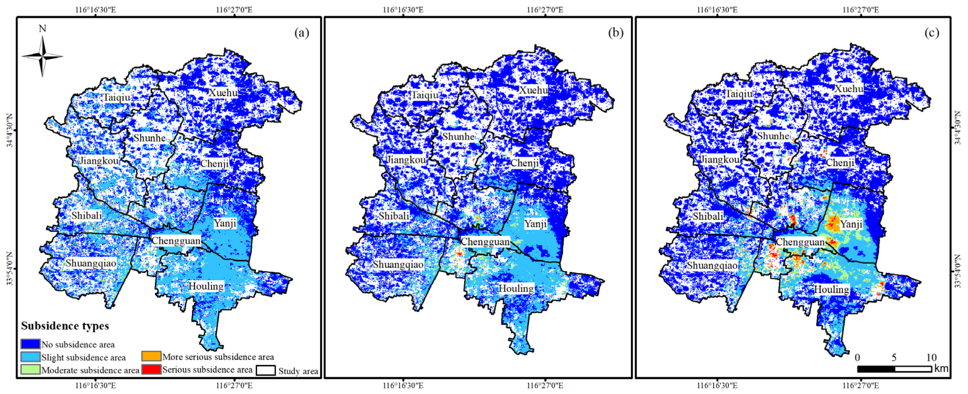
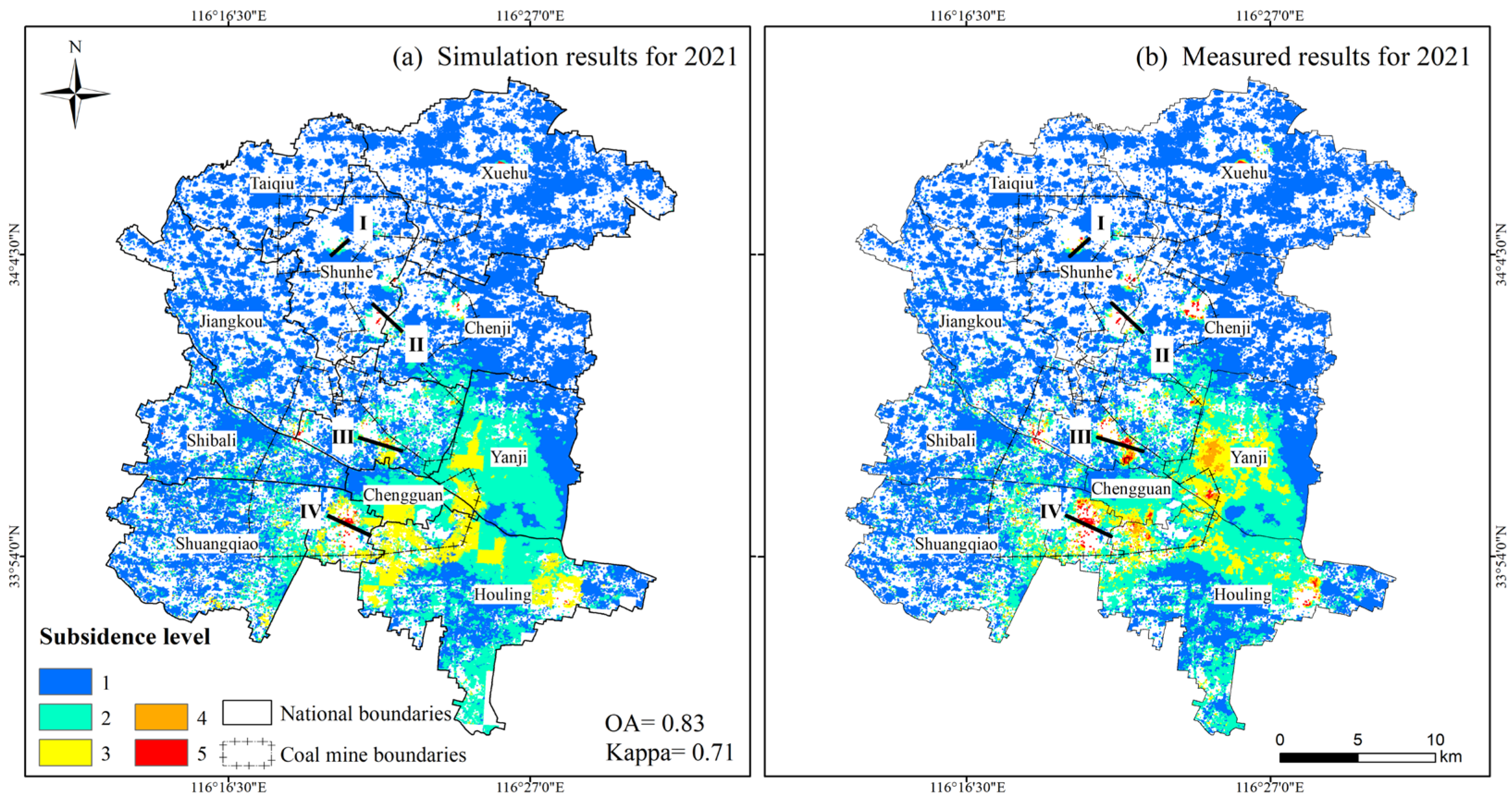
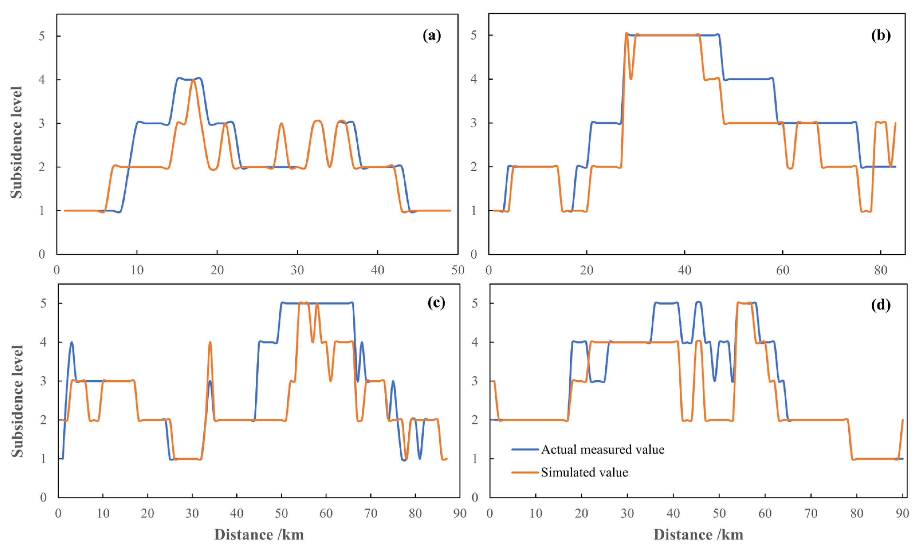
3.3. Spatial and Temporal Simulation of Mining Subsidence

The mining subsidence in 2021 was simulated according to the RF-CA model. In terms of the overall subsidence spatial distribution within the study region, the simulation results are highly consistent with the actual subsidence distribution (Figure 7); the OA is 0.83, and KC is 0.71, indicating that the present method performs well in the simulation of subsidence areas. Although there are some discrepancies, these mainly exist in the urban area, which may be caused by the absence of certain driving factors in the CA model and the spatio-temporal evolution of subsidence in an unnatural state caused by urban planning.

Aiming to better verify the applicability of the model and the accuracy of the local simulation, we selected and plotted four cross-sections (I, II, III, and IV) at different locations within the mining area, as presented in Figure 7. Figure 8 illustrates that the fitting accuracy of the actual measured subsidence values and the simulated subsidence values in the four profiles are high, and the overall accuracy is higher than 0.8. This indicates that the constructed RF-CA spatial–temporal prediction model for ground subsidence is able to learn the local features from the subsidence images during the simulation process, and the simulation result is highly reliable.

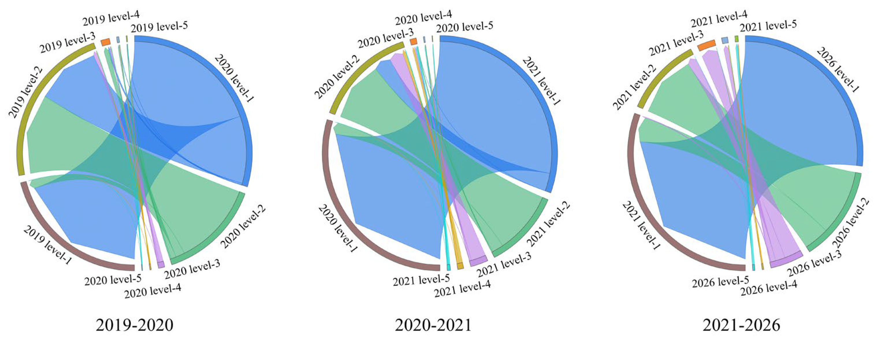
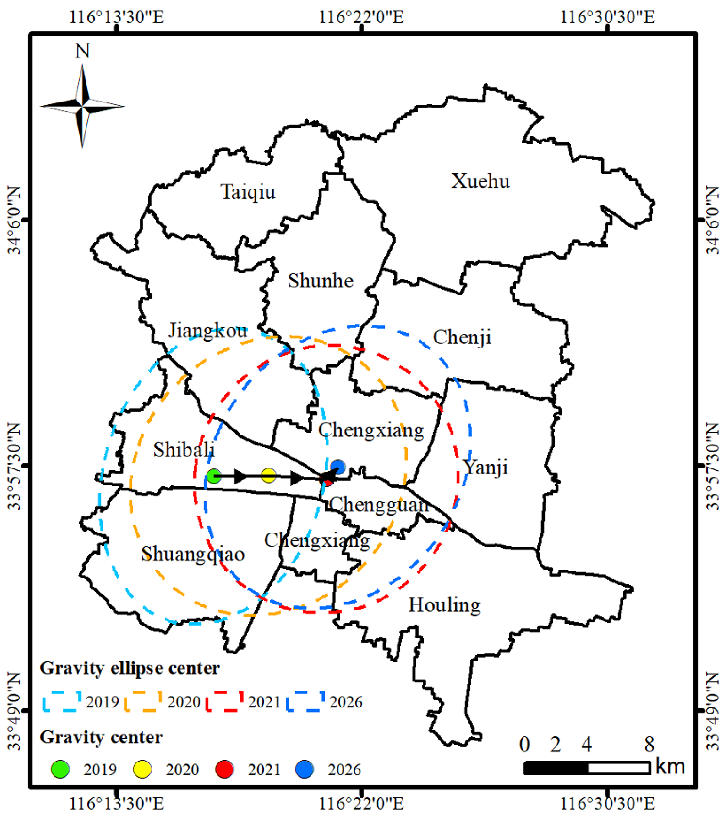
3.4. Trend Analyses of Spatio-Temporal Evolution of Mining Subsidence

Considering the need for model input, the raster data of the subsidence area were transformed into point data, and a kernel density analysis of the subsidence data in 2019–2021 was carried out to obtain the distribution density characteristics of the subsidence region over all three years (Figure 9). It is clear from Figure 9 that the range of the subsidence region progressively expands over time. The subsidence area is mainly concentrated in Xuehu Town in the north of the study region, Chenji Town in the east, and Chengguan Town, Yanji Town, Houling Town, and Chengxiang Township in the southeast.

The area transfer trajectories of different subsidence types were analyzed using the chordal graph visualization model. As shown in Figure 10, the area transfer of slight subsidence and moderate subsidence in the study area was most obvious during 2019–2026, with a total area transfer of 23.71 km² and 7.31 km² (2019–2020), 19.85 km² and 23.26 km² (2020–2021), and 39.13 km² and 24.19 km² (2021–2026), respectively. From 2019 to 2021, the development of subsidence was most intense during this period. The areas of more serious subsidence and serious subsidence increased, and the total area transfer of the two types of subsidence was 8.34 km² and 3.89 km², respectively. By 2026, the total area transfer of more serious subsidence and serious subsidence is projected to decrease by 0.85 km² and 0.13 km², respectively. Though the growth rate of subsidence slows down, subsidence in the region still continues to develop. Considering that coal mining inevitably causes surface subsidence, it is important to formulate a scientific and reasonable surface subsidence prevention and control program to reduce damage from coal mining and for ecological and environmental protection [66].

Using the center of gravity migration model, the change in the overall center of gravity of the subsidence was analyzed in this study area (Figure 11). In the past two years, the center of gravity of the subsidence range did not change substantially and remained near the perimeter of the original subsidence area. During 2019–2021, the center of gravity showed a spatial trend towards the east (2.95 km) and southeast (3.12 km). After 2021, it gradually moved towards the northeast (1.05 km). This movement in the subsidence area is mainly due to the newly introduced working face mining in the mine. In addition, some of the subsidence areas are located in urban regions outside the mine boundaries, and the movement of the subsidence range may be due to human activities and changes in the groundwater level. Huang [67], in his study of the Yongcheng mining area, showed that groundwater needs to be discharged during resource development. In addition, rainfall causes surface water to sink into the ground, leading to changes in the water table and resulting in loose surface soil and the subsidence of the ground surface.

4. Discussion

4.1. Comparison of the Method with Other Model Simulation Results

In an attempt to compare the simulation accuracy of the models, the subsidence evolution was also simulated using the CA and Future Land Use Simulation (FLUS) models (Figure 12). The existing 2021 surface subsidence map was used as a reference to compare the simulation accuracy of the three models. As shown in Figure 12, the FLUS model simulation results had the lowest accuracy with an OA of 0.61 and KC of 0.41. It can be seen that there are more incorrectly simulated image pixels in the CA and FLUS models’ simulation results than in the RF-CA model, and the RF-CA model simulation accuracy (OA 0.83, KC 0.71) is higher than the other two models. The RF-CA model simulation results are generally able to maintain a higher degree of consistency with the actual distribution of subsidence in 2021.

Compared with the CA model, the RF-CA model utilizes the RF model to clarify the driving factors’ contribution to subsidence, excavate the development probability of various types of subsidence, and formulate the conversion rules within the neighborhood of each subsidence unit. The coupled CA model completes the simulation of subsidence under the constraints of the various types of subsidence development probabilities, so simulation accuracy is further improved. The experimental results also further illustrate that the contribution of driving factors should be fully considered when performing subsidence simulation, resulting in the improvement in the surface subsidence simulation accuracy.

4.2. Improvements and Extensions of This Research

Based on this study, we identified several areas for the improvement and extension of subsidence simulation using the RF-CA method:

(1)

Improvement of subsidence-driving factor data. Given the complexity of the mining environment and the difficulty of data collection, the driving factor data are still not comprehensive enough. For example, changes in groundwater levels and the existence of faults may also lead to surface subsidence [67]. In the future, we will consider using remote sensing and contacting the staff of relevant departments to obtain more comprehensive data on subsidence-driving factors to improve the accuracy of subsidence simulation.

(2)

Construction of multilayer cellular space to simulate subsidence. This model can utilize historical subsidence data to train the random forest model, establish the correspondence between the upper mining workings and subsidence, and formulate cellular conversion rules. Since there are cases where multiple coal seams are mined at the same or different times in the mining area, combining object-oriented methods should be considered to construct a multilayer cellular space [36,68]. The conversion rules of the cellular space are adjusted according to the mining order to realize the simulation of subsidence from multiple coal seams.

(3)

Refinement of subsidence-driving factor data. Due to the complex stratigraphic conditions in which coal seams are located, rock formations can be categorized into horizontal, vertical, and thrust faults after structural action [69]. In the future, we could categorize the rock formation of different structures, construct the driving factor dataset separately, and clarify the contribution of the rock formation of different structures to subsidence using this model.

5. Conclusions

In this research, a novel RF-CA model that combines a machine learning algorithm (RF) and the CA model is proposed for subsidence simulation. Based on our method, the contribution of driving factors to mining subsidence is quantitatively described. The method couples the spatial variation in mining subsidence with time while taking into account the contribution of driving factors, which effectively simulates the process of subsidence. The main conclusions are as follows:

(1)

After quantitative analysis, it can be seen that the depth–thickness ratio (0.242), the distance to the working face (0.159), the distance to the building (0.150), and the nature of the rock formation (0.147) always play the main driving roles in subsidence development.

(2)

From the simulation results, it can be seen that the overall trend of subsidence increased during the period 2019–2026. By 2021, more areas of more serious subsidence and serious subsidence occurred, with a total area transfer of 8.34 km² and 3.89 km², respectively. By 2026, the growth trend is predicted to slow down, with a total area transfer of 0.85 km² and 0.13 km², respectively. Overall, the subsidence shows a spatial trend towards the east (2.95 km), southeast (3.12 km), and northeast (1.05 km).

(3)

Compared with other methods, this method is simple to calculate, and there is no requirement to set a large number of simulation parameters artificially. In terms of simulation accuracy, the OA is 0.83, and the KC is 0.71. Due to the limited acquisition of some of the mining data, the impact factors considered are still insufficient, and the simulation accuracy still needs to be improved. In the context of Yongcheng coalfield in China, this study’s results demonstrate the appropriateness and feasibility of the method. The approach can be used to guide the simulation of mining subsidence for other mining areas and can provide technical support for land use planning and environmental conservation protection in coal-resource-based cities.

References

1. Li, Y.; Pan, S.; Ning, S.; Shao, L.; Jing, Z.; Wang, Z. Coal measure metallogeny: Metallogenic system and implication for resource and environment. Sci. China Earth Sci. 2022, 65, 1211–1228. [Google Scholar] [CrossRef]
2. Wang, X. Consideration of building modernized coal economic system. China Coal 2018, 44, 5–8. [Google Scholar] [CrossRef]
3. Wang, S.; Sun, Q.; Geng, J.; Yuan, S.; Jia, H.; Wang, S.; Zhang, W.; Hu, J.; Li, D. Geological Support for Response and Damage Reduction in Earth’s Critical Zone under Coal Mining. Geol. China 2024, 11, 1–22. [Google Scholar] [CrossRef]
4. Cheng, S.; Gu, H.; Song, W.; Ai, Y.; Zhang, Y.; Lu, S. Study on the Ecological Disturbance Monitoring in Mining Area Based on Remote Sensing Information: Taking Qian’an City as an Example. Met. Mine 2021, 5, 182–189. [Google Scholar] [CrossRef]
5. Dai, G.; Xue, X.; Niu, C.; Xu, K.; Jiang, Z.; Xiao, L.; Liu, M. Disturbance characteristics of coal mining to the eco-phreatic flow field in adjacent regions. J. China Coal Soc. 2019, 44, 701–708. [Google Scholar] [CrossRef]
6. Wang, Y. Research Progress and Prospect on Ecological Disturbance Monitoring in Mining Area. Acta Geod. Cartogr. Sin. 2017, 46, 1705–1716. [Google Scholar] [CrossRef]
7. Li, Q.; Hu, Z.; Zhang, F.; Guo, Y.; Liang, Y. A Study on Historical Big Data Analysis of Surface Ecological Damage in the Coal Mining Area of Lvliang City Based on Two Mining Modes. Land 2024, 13, 1411. [Google Scholar] [CrossRef]
8. Litwiniszyn, J. Stochastic methods in subsidence problems: Proc International Symposium on Modern Mining Technology, Taian, October 1988 P300-305. Publ Taian: Shandong Institute of Mining and Technology, 1988. Int. J. Rock Mech. Mech. Min. 1990, 27, 300–305. [Google Scholar] [CrossRef]
9. Álvarez-Fernández, M.I.; González-Nicieza, C. Generalization of the n-k influence function to predict mining subsidence. Eng. Geol. 2005, 80, 1–36. [Google Scholar] [CrossRef]
10. Nicieza, C.G.; Fernandez, M.I.A.; Diaz, A.M. The new three-dimensional subsidence influence function denoted by n-k-g. J. Rock. Mech. Mech. Min. 2005, 42, 372–387. [Google Scholar] [CrossRef]
11. Behrooz, G.; Kazem, G.; Gang, R.; John, V. Numerical modelling of multistage caving processes: Insights from multi-seam longwall mining-induced subsidence. Int. J. Numer. Anal. Met. 2017, 41, 959–975. [Google Scholar] [CrossRef]
12. Alam, A.; Badrul Fujii, Y.; Eidee, S.; Boeut, S.; Rahim, A. Prediction of mining-induced subsidence at Barapukuria longwall coal mine, Bangladesh. Sci. Rep. 2022, 12, 14800. [Google Scholar] [CrossRef] [PubMed]
13. Jeon, B.; Jeong, H.; Choi, S.; Jeon, S. Assessment of Subsidence Hazard in Abandoned Mine Area Using Strength Reduction Method. KSCE J. Civ. Eng. 2022, 26, 4338–4358. [Google Scholar] [CrossRef]
14. Xu, X.; Zhou, C.; Gong, H.; Chen, B.; Wang, L. Monitoring and Analysis of Land Subsidence in Cangzhou Based on Small Baseline Subsets Interferometric Point Target Analysis Technology. Land 2023, 12, 2114. [Google Scholar] [CrossRef]
15. Ferretti, A.; Prati, C.; Rocca, F. Permanent scatterers in SAR interferometry. IEEE Trans. Geosci. Remote Sens. 2001, 39, 8–20. [Google Scholar] [CrossRef]
16. Blachowski, J.; Milczarek, W.; Grzempowski, P. Application of psinsar for assessment of surface deformations in post-mining area-case study of the former walbrzych hard coal basin (sw poland). Acta Geodyn. Geomater. 2017, 14, 41–52. [Google Scholar] [CrossRef]
17. Zhang, W.; Zhang, T.; Zhang, F. Identification of ground subsidence in goaf of Hancheng Mining Area based on PS-InSAR and DS-InSAR. Saf. Coal Mines 2022, 53, 194–199. [Google Scholar] [CrossRef]
18. Yang, X.; Niu, Y.; Zhang, Z.; Zhang, P.; Liu, K.; Zhang, L. Research on subsidence monitoring of SBAS-InSAR mining area based on UAV DEM fusion: A case study of a mining area in Wu’an. Prog. Geophys. 2024, 39, 0038–0047. [Google Scholar] [CrossRef]
19. Wang, X.; Du, Y.; Jiang, J.; Zhao, F.; Yan, S. Monitoring of temporal and spatial evolution of surface deformation in Yuncheng Mining Area with DS-InSAR. Saf. Coal Mines 2021, 52, 120–125. [Google Scholar] [CrossRef]
20. Yang, Y.; Zhang, S.; Hou, H.; Li, X. The Ecological Impacts of Coal Mining and the Regional Differentiation. China Land Sci. 2015, 29, 55–62. [Google Scholar] [CrossRef]
21. Arsanjani, J.; Helbich, M.; Kainz, W.; Boloorani, A. Integration of logistic regression, Markov chain and cellular automata models to simulate urban expansion. Int. J. Appl. Earth Obs. 2013, 21, 265–275. [Google Scholar] [CrossRef]
22. Chen, Y.; Li, X.; Liu, X.; Ai, B. Modeling urban land-use dynamics in a fast developing city using the modified logistic cellular automaton with a patch-based simulation strategy. Int. J. Geogr. Inf. Sci. 2014, 28, 234–255. [Google Scholar] [CrossRef]
23. Tang, Z.; Mei, Z.; Liu, W.; Xia, Y. Identification of the key factors affecting Chinese carbon intensity and their historical trends using random forest algorithm. J. Geogr. Sci. 2020, 30, 743–756. [Google Scholar] [CrossRef]
24. Zhou, J.; Chen, K.; Yan, X.; Xu, J.; Yan, C.; Feng, H.; Li, Z. Automatic extraction method of loess erosion gullies based on BP neural network. J. Spatio-Temp. Inf. 2023, 30, 193–201. [Google Scholar] [CrossRef]
25. Liu, X.; Liang, X.; Li, X.; Xu, X.; Ou, J.; Chen, Y.; Li, S.; Wang, S.; Pei, F. A future land use simulation model (FLUS) for simulating multiple land use scenarios by coupling human and natural effects. Landsc. Urban Plan. 2017, 168, 94–116. [Google Scholar] [CrossRef]
26. Liang, X.; Liu, X.; Li, D.; Zhao, H.; Chen, G. Urban growth simulation by incorporating planning policies into a CA-based future land-use simulation model. Int. J. Geogr. Inf. Sci. 2018, 32, 2294–2316. [Google Scholar] [CrossRef]
27. Liu, X.; Pei, F.; Wen, Y.; Li, X.; Liu, Z. Global urban expansion offsets climate-driven increases in terrestrial net primary productivity. Nat. Commun. 2019, 10, 5558. [Google Scholar] [CrossRef]
28. Liang, X.; Guan, Q.; Clarke, K.; Liu, S.; Yao, Y. Understanding the drivers of sustainable land expansion using a patch-generating land use simulation (PLUS) model: A case study in Wuhan, China. Comput. Environ. Urban 2021, 85, 101569. [Google Scholar] [CrossRef]
29. Liang, X.; Tian, H.; Li, X.; Huang, J.; Clarke, K.; Yao, Y.; Guan, Q.; Hu, G. Modeling the dynamics and walking accessibility of urban open spaces under various policy scenarios. Landsc. Urban Plan. 2021, 207, 103993. [Google Scholar] [CrossRef]
30. Wang, K.; Xiao, X.; Yu, Y.; Jia, Q.; Zhao, S. Hybrid prediction model of surface subsidence deformation using CEEMDAN-CNNBiLSTM. J. Navig. Position. 2024, 12, 156–163. [Google Scholar] [CrossRef]
31. Liu, J.; Sun, X.; Chen, G.; Li, S.; Jia, P.; Chen, C. Tunnel Vault Settlement Prediction Based on Spatiotemporal Characteristics. J. Xuzhou Inst. Technol. Nat. Sci. Ed. 2024, 39, 11–17. [Google Scholar] [CrossRef]
32. Koreen, M.; Murray, R. On the importance of training data sample selection in random forest image classification: A case study in peatland ecosystem mapping. Remote Sens. 2015, 7, 8489–8515. [Google Scholar] [CrossRef]
33. Silvia, V.; David, M.; Jordi, I. Production of a dynamic cropland mask by processing remote sensing image series at high temporal and spatial resolutions. Remote Sens. 2016, 8, 55. [Google Scholar] [CrossRef]
34. Yang, J.; Hu, T.; Li, B.; Li, D.; Zhang, J.; Huang, Q.; Ge, B.; Bai, T. Spatial and Temporal Evolution Characteristic of Ecological Sensitivity of Dianchi Lake Basin Based on CA-MC Model. J. Yunnan Agric. Univ. (Nat. Sci.) 2023, 38, 894–906. [Google Scholar] [CrossRef]
35. Zhang, D.; Liu, X.; Yao, Y.; Zhang, J. Simulating Spatiotemporal Change of Multiple Land Use Types in Dongguan by Using Random Forest Based on Cellular Automata. Geogr. Geo-Inf. Sci. 2016, 32, 22–28. [Google Scholar]
36. Chen, Q.; Li, J.; Hou, E. Dynamic simulation for the process of mining subsidence based on cellular automata model. Open Geosci. 2020, 12, 832–839. [Google Scholar] [CrossRef]
37. He, C.; Okada, N.; Zhang, Q.; Shi, P.; Li, J. Modelling dynamic urban expansion processes incorporating a potential model with cellular automata. Landsc. Urban Plan. 2008, 86, 79–91. [Google Scholar] [CrossRef]
38. El Kamali, M.; Papoutsis, I.; Loupasakis, C.; Abuelgasim, A.; Omari, K.; Kontoes, C. Monitoring of land surface subsidence using persistent scatterer interferometry technology and ground truth data in arid and semi-arid regions, the case of Remah, UAE. Sci. Total Environ. 2021, 776, 145946. [Google Scholar] [CrossRef]
39. Berardino, P.; Fornaro, G.; Lanari, R.; Sansosti, E. A new algorithm for surface deformation monitoring based on small baseline differential SAR interferograms. IEEE Trans. Geosci. Remote Sens. 2002, 40, 2375–2383. [Google Scholar] [CrossRef]
40. Ma, D.; Guan, Y.; Zhao, S. Monitoring of Surface Deformation in Xi-shan Coalfield Area of Shanxi Province Based on SBAS-InSAR Technology. Coal Technol. 2021, 40, 130–135. [Google Scholar] [CrossRef]
41. Xu, J.; Yan, C.; Boota, M.; Chen, X.; Li, Z.; Liu, W.; Yan, X. Research on automatic identification of coal mining subsidence area based on InSAR and time series classification. J. Clean. Prod. 2024, 470, 143293. [Google Scholar] [CrossRef]
42. Zhu, J.; Li, Z.; Hu, J. Research Progress and Methods of InSAR for Deformation monitoring. Acta Geod. Cartogr. Sin. 2017, 46, 1717–1733. [Google Scholar] [CrossRef]
43. Liu, L.; Wang, Z.; Liang, Z.; Liu, Y. Importance analysis of building components for earthquake losses based on the random forest algorithm. Earthq. Eng. Eng. Dyn. 2024, 44, 70–78. [Google Scholar]
44. Guo, R.; Wu, T.; Wu, X.C.; Luigi, S.; Wang, Y.Q. Simulation of urban land expansion under ecological constraints in Harbin-Changchun urban agglomeration, China. Chin. Geogr. Sci. 2022, 32, 438–455. [Google Scholar] [CrossRef]
45. Zhou, L.; Dang, X.; Sun, Q.; Wang, S. Multi-scenario simulation of urban land change in Shanghai by random forest and CA-Markov model. Sustain. Cities Soc. 2020, 55, 102045. [Google Scholar] [CrossRef]
46. Biau, G.; Scornet, E. A Random Forest Guided Tour. arXiv 2015. [Google Scholar] [CrossRef]
47. Kavzoglu, T.; Teke, A. Predictive Performances of ensemble machine learning algorithms in landslide susceptibility mapping using random forest, extreme gradient boosting (XG Boost) and natural gradient boosting (NG Boost). Arab. J. Sci. Eng. 2022, 47, 7367–7385. [Google Scholar] [CrossRef]
48. Jiang, Z.; Wang, M.; Liu, K. Comparisons of convolutional neural network and other machine learning methods in landslide susceptibility assessment: A case study in Pingwu. Remote Sens. 2023, 15, 798. [Google Scholar] [CrossRef]
49. Hu, L.; Yan, C. Evaluation of Landslide Susceptibility of Mangshan Mountain in Zhengzhou Based on GWO-1D CNN Model. Sustainability 2024, 16, 5086. [Google Scholar] [CrossRef]
50. Chen, X.; Wang, Z.; Yang, H.; Ford, A.; Dawson, R. Enhanced urban growth modelling: Incorporating regional development heterogeneity and noise reduction in a cellular automata model—A case study of Zhengzhou, China. Sustain. Cities Soc. 2023, 99, 104959. [Google Scholar] [CrossRef]
51. Brendel, A.; Ferrelli, F.; Piccolo, M.; Perillo, G. Assessment of the effectiveness of supervised and unsupervised methods: Maximizing land-cover classification accuracy with spectral indices data. J. Appl. Remote Sens. 2019, 13, 014503. [Google Scholar] [CrossRef]
52. Zhan, Y.; Shakir, M.; Hao, P.; Niu, Z. The effect of EVI time series density on crop classification accuracy. Optik 2017, 157, 1065–1072. [Google Scholar] [CrossRef]
53. Huang, W.; Li, Q.; Jing, W.; Ge, Y.; Dong, P.; Fan, L. Diagnostic Performance of Artificial Intelligence on Benign andMalignant Pulmonary Nodules Under Different WHO Pathological Classifications of Lung Cancer. J. Clin. Radiol. 2025, 44, 76–82. [Google Scholar]
54. Chen, H.; Xu, H.; Li, X.; Mei, X. Research on saliency target recognition in low light images based on dual branch convolutional neural networks. Laser J. 2024, 45, 136–140. [Google Scholar] [CrossRef]
55. Di, Q.; Chen, X.; Wang, M. Spatiotemporal differences and evolutionary trends of coastal marine ecological welfare performance in China. Mar. Sci. Bull. 2022, 41, 302–314. [Google Scholar] [CrossRef]
56. Ma, G.; Liu, T.; Zhang, G. Spatial Evolution and Motivation of Ningbo’s Marine Industry Considering Sub-industries. Geogr. Geo-Inf. Sci. 2024, 40, 141–152. [Google Scholar]
57. Tang, R.; Li, F. Spatiotemporal evolution of cultivated land on basin scale. J. Water Resour. Water Eng. 2024, 35, 87–197. [Google Scholar] [CrossRef]
58. Lei, T.; Wan, S.; Wu, Y.; Wang, H.; Hsieh, C. Multi-temporal data fusion in MS and SAR Images using the dynamic time warping method for paddy rice classification. Agriculture 2022, 12, 77. [Google Scholar] [CrossRef]
59. Feng, J.; Yang, Z.; Xu, Y.; Chen, H. Land subsidence monitoring in coal mining collapse area of Urumqi. GNSS World China 2023, 48, 44–51. [Google Scholar] [CrossRef]
60. Zhang, S.; Zhao, P.; Wang, N.; Zhao, S.; Li, L.; Song, R.; Zhao, W.; Ma, L. Subsidence monitoring of Huainan coal mining area based on Sentinel-1 data integration of DInSAR and SBAS. Chin. J. Geol. 2023, 58, 1521–1534. [Google Scholar] [CrossRef]
61. Gao, J.; Chen, B.; Feng, Z. A Maximum Detectable Deformation Gradient Model of InSAR Technique for Mining Subsidence. Met. Mine 2020, 03, 168–176. [Google Scholar] [CrossRef]
62. Li, Q.; Li, G.; Yang, Z. Study on the influence of the depth/thickness ratio on the ground deformation. In Proceedings of the 2011 International Conference on Consumer Electronics, Communications and Networks (CECNet), Xianning, China, 16–18 April 2011; pp. 1730–1733. [Google Scholar]
63. Guo, W.; Ma, Z.; Bai, E. Current status and prospect of coal mining technology under buildings, water bodies and railways, and above confined water in China. Coal Sci. Technol. 2020, 48, 16–26. [Google Scholar] [CrossRef]
64. Guo, W.; Hu, Y.; Hu, C.; Li, L.; Wu, D.; Ge, Z. System and engineering practice of coal mining technology under buildings, water bodies and railways in China. Coal Sci. Technol. 2024, 9, 1–21. [Google Scholar] [CrossRef]
65. Sun, Q.; Chen, Q.; Mu, Y.; Li, H. Probability integral method for fully mechanized mining in shallow coal seam. Coal Eng. 2023, 55, 146–150. [Google Scholar]
66. Wang, S.; Geng, J.; Li, P.; Sun, Q.; Fan, Z.; Li, D. Construction of geological guarantee system for green coal mining. Coal Geol. Explor. 2023, 51, 33–43. [Google Scholar] [CrossRef]
67. Huang, X. Study on the Development of Land Resources in Mine Subsidence Area. Master’s Thesis, Henan University, Kaifeng, China, 2015. [Google Scholar]
68. Chen, Q. Simulation of Coal Mining Subsidence Based on the Model of Cellular Automata. Sci. Technol. Rev. 2013, 31, 65–67. [Google Scholar]
69. Guo, L.; Kang, X. Study on the stress evolution law of surrounding rock in fault-bearing coal seam group mining. Coal Techn. 2021, 40, 8–11. [Google Scholar] [CrossRef]
Figure 1. Flow chart of spatio-temporal subsidence simulation.
Land 14 00268 g001
Figure 2. Data processing procedure for InSAR technology.
Land 14 00268 g002
Figure 3. Results after reclassification of foundation subsidence data. (ac) represent the corresponding subsidence images for 2019–2021, respectively.
Land 14 00268 g003
Figure 4. Geographic location map of the study area. (a) China; (b) Henan Province, China; (c) Yongcheng coalfield.
Land 14 00268 g004
Figure 5. Heat map of Pearson correlation coefficients of driving factors.
Land 14 00268 g005
Figure 6. Contribution of driving factors.
Land 14 00268 g006
Figure 7. Verification of simulation result accuracy. Numbers 1–5 represent no subsidence, slight subsidence, moderate subsidence, more serious subsidence, and serious subsidence, respectively. I, II, III, and IV represent four cross-sections.
Land 14 00268 g007
Figure 8. Analysis of local simulation accuracy in this study area. (ad) represent the four cross-sections (I, II, III, and IV).
Land 14 00268 g008
Figure 9. Density distribution map of mining subsidence area.
Land 14 00268 g009
Figure 10. Trajectory of change in area of different types of subsidence for the years 2019–2026. Level-1 to Level-5 indicate the different levels of subsidence, respectively.
Land 14 00268 g010
Figure 11. Maps of center of gravity migration in subsidence areas.
Land 14 00268 g011
Figure 12. Comparison of simulation results obtained using different methods. (a1,b1,c1) are the RF-CA, CA, and FLUS model simulation results, respectively, and 1–5 represent no subsidence, slight subsidence, moderate subsidence, more serious subsidence, and serious subsidence, respectively; (a2,b2,c2) are the mis-simulated regions in the simulation results.
Land 14 00268 g012