Abstract
Against the global biodiversity crisis, arid and semi-arid regions are sensitive indicators of terrestrial ecosystems. However, research on their habitat quality (HQ) evolution mechanism faces dual challenges: insufficient multi-scale dynamic simulation and fragmented driving mechanism analysis. To address these gaps, this study takes northern China’s arid and semi-arid regions as the object, innovatively constructing a “pat-tern-process-mechanism” multi-dimensional integration framework. Breaking through single-model/discrete-method limitations in existing studies, it realizes full-process integrated research on regional HQ spatiotemporal dynamics. Based on 1990–2020 Land Use and Land Cover Change (LUCC) data, the framework integrates the InVEST and PLUS models, solving poor continuity between historical assessment and future projection in traditional research. It also pioneers combining the XGBoost-SHAP model and Geographically and Temporally Weighted Regression (GTWR): XGBoost-SHAP quantifies nonlinear interactive effects of natural, socioeconomic, and landscape drivers, while GTWR explores spatiotemporal heterogeneous mechanisms of landscape pattern evolution on HQ, effectively addressing the dual challenges. Results show the following: (1) In 1990–2020, cultivated and construction land expanded, with grassland declining most notably; (2) Overall HQ decreased by 0.82%, with high-value areas stable in the west and northeast, low-value areas concentrated in the central region, and 2030 HQ optimal under the Ecological Protection (EP) scenario; (3) Natural factors contribute most to HQ change, followed by socioeconomic factors, with landscape indices being least impactful; (4) Under future scenarios, landscape Patch Density (PD) has the most prominent negative effect—its increase intensifies fragmentation and reduces connectivity. This study’s method integration breakthrough provides a quantitative basis for landscape pattern optimization and ecosystem management in arid and semi-arid regions, with important scientific value for promoting integration of landscape ecology theory and sustainable development practice.
1. Introduction
Ecosystems, the core components of Earth’s life-support system, are indispensable for sustaining human society through environmental security, resource provision, and global biogeochemical regulation, while delivering critical ecological functions such as climate modulation, carbon sequestration, and soil–water conservation [1,2]. Habitat quality (HQ), a synthetic measure of ecosystem service (ES) capacity, reflects the structural integrity and functional stability of regional ecosystems, serving as a pivotal metric for evaluating the sustainability of human–nature coupled systems [3,4]. Over the past four decades, ecosystem degradation—driven by climate change and anthropogenic pressures—has emerged as a global crisis, with Intergovernmental Science-Policy Platform on Biodiversity and Ecosystem Services (IPBES) assessments revealing that 75% of terrestrial ecosystems are significantly degraded and over 1 million species face extinction risks, a trend acutely manifested in arid zones [5]. China’s arid and semi-arid regions (ASAR), vital ecological barriers for Eurasia, exemplify this challenge: despite covering 30% of the nation’s land area, they hold only 4% of its water resources [6], exacerbating ES decline. Remote sensing data further indicate Normalized Difference Vegetation Index (NDVI) growth rates below the national average in 1990–2020, compounded by spatially heterogeneous landscape fragmentation [7]. Consequently, reconciling HQ enhancement with socioeconomic development through landscape planning has become a frontier in arid-region sustainability research [8,9].
The paradigm of HQ research has evolved from disciplinary silos to multidisciplinary integration, mirroring advances in ecological methodologies and theoretical frameworks. Early studies relied on biologists’ plot-scale observations of indicator species or communities [10], offering limited insights into regional ecosystem dynamics. The advent of remote sensing, Geographic Information System (GIS), and ecological modeling has since enabled systematic assessments through multi-source data fusion, process-based simulations, and spatiotemporal analysis [11,12], shifting the focus from static descriptions to dynamic predictions. Next-generation models (e.g., InVEST, HSI) now integrate multi-scale data to refine HQ simulations [13], facilitating quantitative ES evaluations from landscapes to regions. Crucially, land use/cover change (LUCC), as the spatial footprint of human activity [14], has emerged as a key lens for deciphering human–environment interactions. Landscape patterns—imprints of long-term natural–anthropogenic interplay—exert multilevel influences on HQ by modulating material, energy, and information flows [15]: microscale fragmentation disrupts species migration and genetic exchange [16]; mesoscale alterations affect ES flows [17]; and macroscale shifts redefine ecological security patterns [18]. These impacts exhibit nonlinearity—moderate heterogeneity supports biodiversity, whereas excessive fragmentation erodes ecosystem functionality.
Habitat quality is shaped by a complex interplay of climatic variables and human activities that directly modify land cover and species interactions [19]. Human-induced land use activities exert a direct impact on the link between ecosystem structure and function—an influence that is particularly pronounced in arid and semi-arid basins, where fragile ecological backgrounds render such systems highly sensitive to anthropogenic disturbances. Against this backdrop, the systematic evaluation of Habitat Quality (HQ) serves as critical evidence for diagnosing the health status of these vulnerable ecosystems and advancing the sustainability of arid and semi-arid areas. Additionally, quantifying the spatiotemporal responses of HQ to changes in Land Use and Land Cover (LULC) facilitates the identification of conservation priorities across the basin. This, in turn, provides support for evidence-based strategies aimed at reconciling ecological resilience with the pressing demands of socioeconomic development. Key drivers include climatic extremes that exacerbate habitat fragmentation and species mortality [20,21,22], as well as land-use changes that diminish natural habitats and intensify fragmentation. However, current research lacks long-term mechanistic insights into these drivers, and the nonlinear interactions among explanatory variables challenge conventional models in identifying dominant factors and their interdependencies. This gap in driving mechanism analysis is not trivial: without clarifying how natural, socioeconomic, and landscape factors interact nonlinearly to shape HQ, managers cannot design targeted interventions. Machine learning (ML) algorithms, renowned for handling complex nonlinearities [23], offer promising solutions. Recent studies have leveraged ML techniques such as random forest (RF), XGBoost, and boosted regression trees (BRT) to enhance predictive accuracy [24,25,26]. Complementing these, Shapley additive explanations (SHAP) transcend “black-box” limitations by quantifying variable contributions and elucidating interaction effects [27].
Concurrently, advances in spatiotemporal prediction, critical for ecological planning and land restoration, underscore the importance of long-term LUCC simulations [28]. While traditional models (e.g., CA-Markov, CLUE-S, FLUS) struggle with patch-scale dynamics and spatiotemporal fidelity, the PLUS model outperforms them in accuracy, enabling robust scenario analyses—from assessing ecosystem service value (ESV) impacts [29] to predicting wetland distribution shifts [30]. The lack of detailed multi-scale dynamic simulations in existing ASAR research poses a practical barrier: arid ecosystems are highly sensitive to subtle changes in land use and climate, and without integrating microscale fragmentation, mesoscale, and macroscale into a unified simulation framework, projections of future HQ remain coarse and unreliable. This undermines the scientific basis for policies such as the “Three Norths” Shelterbelt Program, which requires precise spatial-temporal guidance to allocate restoration resources effectively. Against the backdrop of global biodiversity decline, ASAR—as sensitive terrestrial ecosystem indicators—face pressing research gaps in multi-scale HQ dynamics and fragmented driver analyses. This study addresses these gaps through three objectives: (1) employing high-resolution LUCC data (1990–2020) and the InVEST model to quantify spatiotemporal HQ heterogeneity; (2) leveraging the PLUS model to simulate 2030 land-use evolution under natural development (ND), ecological preservation (EP), and cropland preservation (CP) scenarios, overcoming single-scale limitations; (3) integrating XGBoost-SHAP to quantify driver contributions (natural, socioeconomic, landscape) and applying GTWR to dissect spatial heterogeneity mechanisms linked to future landscape patterns.
2. Materials and Methods
2.1. Study Area
The ASAR of China represent a vast and ecologically significant zone, extending from areas west of the Daxing’anling Mountains in the northeast to territories north of the Qinghai–Tibetan Plateau and Loess Plateau. Encompassing four provincial-level administrative regions (Xinjiang, Gansu, Ningxia Hui Autonomous Region, and Inner Mongolia), this expansive area spans approximately 3.23 × 10⁶ km2, constituting about one-third of China’s total land area (Figure 1). Despite its geographical expanse, the region supports only about 4% of the nation’s population. Characterized by substantial altitudinal variation and generally high elevations, this deeply continental zone experiences minimal monsoon influence, resulting in pronounced climatic gradients. Annual precipitation decreases sharply from approximately 400 mm in eastern areas to less than 100 mm in western regions, while temperatures range from −33 °C to 17 °C annually, with marked diurnal fluctuations. Dominated by desert vegetation and nutrient-poor soils interspersed with fragmented grassland ecosystems, the region exhibits exceptional ecological fragility. Water scarcity represents a fundamental constraint on agricultural development, particularly in eastern monsoon-affected areas where ecosystems demonstrate heightened sensitivity to anthropogenic disturbance. Unsustainable land use practices, notably overgrazing, have significantly exacerbated desertification risks throughout this vulnerable region. The study area is confronted with severe desertification and fragile desert ecosystems, with per capita water resources accounting for less than 1/5 of the national average [31]. Due to scarce perennial precipitation, issues such as ecological vulnerability, reduced vegetation cover, population growth, and soil erosion—exacerbated by climate warming and aridification—have become increasingly prominent, restricting the region’s ecological environment and socio-economic development [32]. The long-term arid trend, coupled with intensive agriculture and grazing, has led to reduced runoff in rivers, lakes, and reservoirs within the basin, as well as groundwater depletion. Challenges including water scarcity, climate change, and soil erosion have further aggravated grassland degradation, rendering the ASAR ecosystem increasingly fragile.
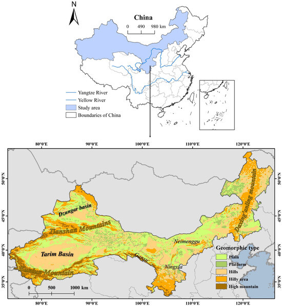
Figure 1.
Geographic location of the study area.
2.2. Data Sources
This study integrated multi-source spatial datasets, standardized to a 1 km resolution and clipped to the arid and semi-arid region boundaries, to ensure analytical consistency. Land use/cover maps (1990–2020), socioeconomic metrics (GDP, population density), and administrative boundaries were sourced from the Chinese Academy of Sciences’ Resource and Environmental Science Data Center (RESDC). Terrain parameters derived from NASA’s SRTM1 v3.0 elevation data and climatic variables (temperature, precipitation) from the National Earth System Science Data Center were complemented by evapotranspiration data (National Tibetan Plateau Data Center) and infrastructure layers (OpenStreetMap). Additional ecological indicators—including NDVI and nighttime light data—were acquired from the Geographic Remote Sensing Ecological Network Platform, with hydrological references provided by the National Geomatics Center of China (Table 1).

Table 1.
Data sources.
2.3. Methodology
This study developed an integrated framework for HQ assessment through a multi-method analytical approach. First, land use/cover change (LUCC) dynamics in ASAR (1990–2020) were analyzed, quantifying transition processes using transfer matrices. Second, the InVEST model’s HQ module was employed to evaluate spatiotemporal patterns by integrating ecosystem sensitivity and threat factor distributions. Building on these historical assessments, the PLUS model was coupled to project 2035 land use patterns under three scenarios: natural development (ND), ecological protection (EP), and cropland protection (CP), enabling multi-scenario HQ predictions. Third, Fragstats software was utilized to compute class- and landscape-level indices, applying the moving window method to characterize spatiotemporal changes in landscape heterogeneity. Finally, the XGBoost-SHAP model was implemented to identify key driver contributions and their interaction effects, complemented by spatiotemporal geographically weighted regression (GTWR) to quantify spatial relationships between landscape pattern indices and HQ under future scenarios (Figure 2).
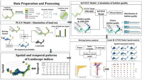
Figure 2.
Research framework.
2.3.1. Habitat Quality (HQ)
The Integrated Valuation of Ecosystem Services and Trade-offs (InVEST) model is a widely used quantitative assessment tool jointly developed by Stanford University and the World-Wide Fund for Nature in 2007, designed to bridge ecological science and decision-making by quantifying ecosystem services and their spatial patterns [33,34]. Distinguished by its modular design, user-friendly interface, and minimal data input requirements, the model supports comprehensive evaluations across terrestrial, freshwater, and marine ecosystems, with core modules covering habitat quality, carbon storage, water yield, soil conservation, and coastal protection [35]. The Integrated Valuation of ESs and Trade-offs (InVEST) model serves as a robust analytical tool for ecosystem assessment [36], particularly for evaluating biodiversity functionality through HQ quantification [37,38]. This model uniquely incorporates anthropogenic disturbance factors, enabling precise assessment of human impacts on ecosystem integrity. Version 3.12.0 of the InVEST model was implemented to assess HQ in China’s ASAR, employing a sophisticated algorithm that integrates landscape type sensitivity with external threat intensity. The model generates HQ (HQ) indices scaled from 0 to 1, where higher values correspond to superior ecological conditions. The HQ calculation follows this formulation:
The HQ for land grid x of category j is calculated as a function of three key components: representing the habitat suitability score, quantifying the degree of threat exposure, and as the half-saturation constant (typically set at half the maximum habitat degradation value). The threat coefficient specifically measures habitat stress from external disturbances, including anthropogenic pressures and natural disasters, where higher values indicate greater ecological threat and consequently poorer HQ. Model parameters were carefully calibrated according to the InVEST modeling manual and established literature, with cropland, constructed land, and unutilized land identified as primary threat factors [39,40,41]. The spatial analysis incorporated multi-temporal raster data of threat factor distributions along with weighted sensitivity tables for each threat source. Complete specifications of threat factor weightings and habitat type sensitivities are provided in Supplementary Materials Tables S1 and S2.
2.3.2. Landscape Pattern Indices (LSPIs)
Landscape pattern indices (LSPIs) serve as crucial quantitative measures for characterizing spatial configurations and temporal evolution of landscape structures [42]. In this study, a multi-dimensional analytical framework focusing on aggregation, connectivity, and diversity dimensions was employed to assess landscape-level changes. Following the principles of minimal correlation and maximal coverage, six representative indices were selected: the largest patch index (LPI) for dominance analysis, patch cohesion index (COHESION) for connectivity assessment, patch density (PD) for fragmentation evaluation, aggregation index (AI) for spatial clustering, contagion index (CONTAG) for dispersion patterns, and Shannon’s diversity index (SHDI) for heterogeneity quantification.
All indices were calculated using Fragstats 4.2 software. Fragstats is a widely used, comprehensive software tool specifically designed for the quantification and analysis of landscape patterns across multiple spatial scales, including patch, class, and landscape levels [43]. Developed to process raster or vector land use/cover data, it enables the calculation of over 100 landscape metrics that characterize key attributes such as composition and configuration. These metrics provide critical insights into how spatial patterns of ecosystems are structured and how they may influence ecological processes like species migration, resource flow, and habitat quality [44]. While previous studies have attempted to integrate multiple indices into composite fragmentation measures [45,46], the inherent dimensional differences among indices often compromise comparability. To address this limitation, a normalization procedure followed by weighted map algebra was implemented to generate a standardized composite fragmentation index, expressed as follows:
The normalization procedure transforms landscape indices into comparable, dimensionless values ranging from 0 to 1. For a given landscape index X, the normalized value is calculated differently depending on the index’s ecological interpretation: positive indicators (where higher values denote favorable conditions) employ Equation (2), while negative indicators (where higher values suggest degradation) utilize Equation (3). Here, Max and Min represent the respective maximum and minimum values observed in the study region’s sample data. This dual-equation approach ensures proper directionality in the normalization process, maintaining the ecological meaning of each index while enabling their integration into a composite fragmentation measure.
2.3.3. PLUS Model
Land use change simulation represents a critical methodological approach for predicting spatial-temporal patterns of landscape transformation [47]. While traditional cellular automata (CA) and CLUE-S models have been widely applied, their limitations in handling patch dynamics and policy scenarios prompted the development of the Patch-generating Land Use Simulation (PLUS) model [48]. The PLUS model innovatively combines Land Expansion Analysis Strategy (LEAS) and CA with multiple stochastic patch seeding mechanisms (CARS), significantly improving simulation accuracy for land use patches under various policy constraints. By incorporating artificial neural networks (ANNs) to analyze natural and socioeconomic drivers, PLUS effectively addresses the complex nonlinearities in land type conversions [49].
In this study, the PLUS model was implemented to simulate 2030 land use patterns across China’s ASAR under three distinct scenarios. Model validation yielded a Kappa coefficient of 0.82, confirming high reliability for regional applications. The scenario framework includes the following: (1) Natural Development (ND), projecting trends through Markov chain transitions of historical patterns; (2) Ecological Protection (EP), prioritizing ecosystem integrity through 15–20% reduced conversion probabilities of natural lands to built-up areas; (3) Cropland Protection (CP), safeguarding food security via 15–30% restrictions on prime farmland conversion [50,51]. The ND scenario assumes system-endogenous growth absent policy interventions, while EP and CP scenarios incorporate targeted constraints reflecting sustainable development priorities.
2.3.4. XGBoost Model
Machine learning has emerged as a transformative approach in urban and environmental studies, overcoming key limitations of traditional analytical methods. Among these techniques, the XGBoost algorithm has demonstrated particular efficacy, establishing itself as a powerful tool for both regression and classification tasks across diverse disciplines including geology, hydrology, and ecology [52,53,54]. This algorithm exhibits several superior characteristics compared to alternative methods like Random Forest (RF) and Gradient Boosting Decision Tree (GBDT): (1) enhanced robustness when handling missing values and large-scale datasets [55], (2) effective management of multicollinearity issues, and (3) improved predictive accuracy through iterative decision tree construction and loss function optimization. The mathematical formulation of its objective function can be expressed as follows:
The objective function on the left side of Equation (4) integrates two key components to balance the model’s prediction accuracy and generalization ability. It consists of the sum of the loss function for all N samples and the sum of the regularization term for all K trees. Specifically, the loss function quantifies the error between the model’s predicted value and the true label , ensuring the model fits the training data effectively. Where is the loss function, which represents the error between the model’s predicted value and the true label . is the regularization term, which is used to control the complexity of the model; is the number of samples and is the number of trees. We modeled the samples of the machine learning model by dividing them into a training dataset (80%) and a test dataset (20%), set a random number seed, and optimized the hyperparameters of the model (e.g., max_depth, learning_rate, and nrounds, etc.) in order to evaluate the fitting performance of the model. The evaluation of the accuracy of XGBoost model can be found in Supplementary Materials Table S3.
2.3.5. SHAP
While XGBoost provides valuable feature importance rankings, its capacity to elucidate relationships between predictors and target variables diminishes with increasing dataset complexity. Moreover, the algorithm offers limited insight into the directionality (positive/negative) and functional form of variable effects. The SHAP (Shapley Additive Explanations) framework addresses these limitations by establishing a theoretically grounded approach to feature attribution, derived from cooperative game theory principles. This method quantifies each feature’s marginal contribution to model predictions while accounting for interaction effects among variables [56]. As a post hoc interpretation tool, SHAP values provide three critical advancements: (1) they maintain consistency in feature attribution across different model architectures, (2) they reveal directional impacts (enhancing or suppressing effects) at both global (whole-model) and local (individual prediction) levels, and (3) they uncover nonlinear relationships and threshold effects that conventional importance metrics cannot detect. This multifaceted interpretability makes SHAP particularly valuable for analyzing complex environmental systems where understanding driver interactions is essential for policy and management decisions:
where denotes the predicted value of the model, is the constant term of the model, i.e., the mean of the predicted values of all the training samples, and is the Shapley value of each feature, which represents the contribution of the feature to the final prediction result.
2.3.6. GTWR Model
The Geographic Time-Weighted Regression (GTWR) model represents a significant advancement over traditional Geographic Weighted Regression (GWR) by incorporating temporal dimensions into spatial analysis. This innovative approach addresses critical limitations of both Ordinary Least Squares (OLS) and conventional GWR models through three key capabilities: (1) simultaneous quantification of spatial and temporal relationships among variables, (2) reduction in bias inherent in global regression assumptions, and (3) explicit characterization of spatiotemporal heterogeneity in variable relationships [57]. The GTWR framework captures evolving spatial patterns by allowing regression coefficients to vary across both geographical space and time, providing a more nuanced understanding of dynamic environmental processes. The fundamental relationship is mathematically expressed as:
where m is the total number of samples, , , and are latitude, longitude, and time series, respectively, and sampling point is expressed in spatio-temporal coordinates, is the kth explanatory variable, and is the random error; is the dependent variable, and denotes the th regression coefficient of the th sample point.
This study examines the spatiotemporal impacts of landscape pattern dynamics on HQ through an integrated analytical framework. Using HQ as our dependent variable and landscape pattern indices as explanatory variables, we conducted county-scale analyses following a rigorous statistical protocol. First, covariance testing was performed on all candidate landscape indices using IBM SPSS Statistics (version 27), eliminating highly correlated variables to ensure model robustness. Through this process, three key uncorrelated predictors were identified: the Aggregation Index (AI), Patch Density (PD), and Contagion Index (CONTAG). These selected metrics capture distinct dimensions of landscape configuration while avoiding multicollinearity issues, making them ideal explanatory variables for our spatial regression modeling approach. The AI represents landscape connectivity, PD quantifies fragmentation, and CONTAG measures dispersion patterns—together providing a comprehensive characterization of landscape structure effects on HQ. A summary of the parameters of the GTWR model can be found in Supplementary Materials Table S4.
3. Results
3.1. Changes in Land Use and Landscape Patterns in ASAR of China
3.1.1. Spatial and Temporal Evolution of LUCC 1990–2020
In ASAR, unutilized land and grassland dominate as the primary land types, collectively accounting for over 80% of the total area, followed by arable land, while water bodies and built-up land occupy comparatively smaller proportions (Figure 3). Water bodies are predominantly distributed in high-altitude areas of the southwest and northwest, sustained largely by ice and snow meltwater from mountainous regions, whereas built-up land is concentrated in the eastern and southern zones with higher human activity intensity. Since 1990, cultivated land and built-up land have expanded by 4.36 × 10⁴ km2 and 1.28 × 10⁴ km2, respectively, reflecting growth rates of 18.07% and 67.18%. Conversely, forest land and grassland experienced declines of 9.76 × 10³ km2 (−4.01%) and 1.36 × 10⁴ km2 (−1.15%), respectively. Notably, water bodies and unutilized land saw pronounced reductions, with water body area diminishing by 3.93 × 10⁴ km2 (−21.05%) and unutilized land by 1.89 × 10⁴ km2 (−1.28%).
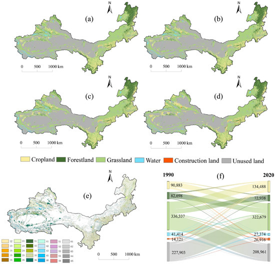
Figure 3.
Distribution and transfer of land-use types in ASAR, 1990–2020 ((a–d) represent the distribution of land use from 1990 to 2020, respectively, (e) shows the spatial transfer of land use in both years, and (f) shows the values of specific transfer changes).
Land use transitions involved approximately 24.57% of the total area, with the most significant exchanges occurring among grassland, unutilized land, and cultivated land. For instance, roughly 3.36 × 10⁴ km2 of grassland was converted, of which 26.49% transitioned to cultivated land, primarily in urbanizing regions of the northeast, northwest, and south. Unutilized land contributed 51.21% of the total transferred area, chiefly in localized areas of Xinjiang and Inner Mongolia, while 57.09% of grassland gains originated from unutilized land. Grassland and cultivated land collectively absorbed 89.8% of the transfers from unutilized land, whereas water bodies and built-up land exhibited minimal outgoing transitions. Overall, grassland served as both the principal source and destination of land transfers, representing over 40% of total transitions in each category (Supplementary Materials Table S5).
3.1.2. Spatial and Temporal Evolution of Landscape Patterns, 1990–2020
Between 1990 and 2020, the landscape pattern index (SHDI) in ASAR exhibited a discernible upward trend (Figure 4), rising from 1.22 to 1.24, signaling heightened diversity and complexity in land-use types and an overall stabilization of the land-use structure. Spatially, elevated SHDI values were concentrated in the eastern and southern regions, characterized by heterogeneous habitat types, as well as around Xinjiang’s Tarim Basin, underscoring their pronounced diversity advantages. In contrast, the CONTAG index displayed an initial decline followed by a modest recovery, decreasing from 48.79 in 1990 to 48.50 in 2020, which reflects a reduction in the dominance of well-connected patches and a concomitant rise in landscape fragmentation. Similarly, the COHESION index stabilized with a marginal decline, suggesting that the connectivity of dominant patches—initially robust—progressively weakened over time. Further reinforcing this trend, the AI index peaked at 82.90 in 2000 before declining to 82.28 by 2020, indicative of a shift from aggregated to more dispersed land-use patterns and a continued deterioration of inter-patch connectivity.
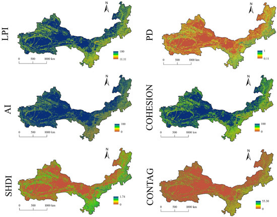
Figure 4.
Characteristics of landscape pattern index distribution in arid and semi-arid zones in 1990.
The landscape pattern analysis reveals distinct trends across different land types. Both cropland and woodland exhibited decreasing patch density (PD) values, suggesting anthropogenic influences on previously continuous patches. Conversely, the increasing PD for water bodies highlights their growing conservation significance in the region. As illustrated in Supplementary Materials Figure S1, unutilized land demonstrated the highest largest patch index (LPI), followed by grassland, confirming their dominance in the study area. While grassland maintained a substantially high LPI and forest land showed minimal changes, all other land types experienced declining LPI values. Notably, cropland exhibited the most pronounced LPI reduction, reflecting significant fragmentation pressures from human activities that necessitate targeted protection strategies. Longitudinal analysis revealed grassland landscapes with the highest landscape shape index (LSI), indicating complex patch geometries associated with ecological stability and resilience, while water bodies showed the lowest LSI values, demonstrating greater vulnerability to anthropogenic disturbances. These findings underscore the urgent need for enhanced protection measures, particularly for aquatic ecosystems and fragmented croplands.
3.2. Spatial and Temporal Evolution of Historical HQ
From 1990 to 2020, HQ in ASAR exhibited a gradual decline, with values decreasing sequentially from 0.5245 to 0.5202 (Figure 5). This downward trend was accompanied by notable shifts in HQ class distribution. While Class I areas decreased from 43.93% to 43.31%, Class II areas showed a more pronounced increase from 7.32% to 8.72%. Class III areas experienced a modest reduction from 39.14% to 38.31%, whereas Class IV areas displayed cyclical fluctuations, initially decreasing before increasing and then decreasing again. Spatially, high-quality habitat zones (Classes III and IV) predominated over low-quality areas (Classes I and II), with distinct geographical patterns emerging. Low-quality Class I zones were primarily located in the central, southwestern, and northwestern regions, characterized by sparse vegetation cover and simplified ecosystem composition, particularly south of the Tianshan Mountains, on the Inner Mongolian Plateau, and in the western study area. In contrast, higher-quality Classes III and IV habitats were concentrated in eastern and northeastern regions, especially in the plains east of the Daxing’anling Mountains. These areas benefited from extensive forest cover and favorable geographic conditions, including flat terrain and abundant water resources, which supported grassland and woodland ecosystems while limiting urban expansion. The spatial distribution of HQ thus reflects a clear interplay between natural vegetation patterns, topographic features, and anthropogenic influences.
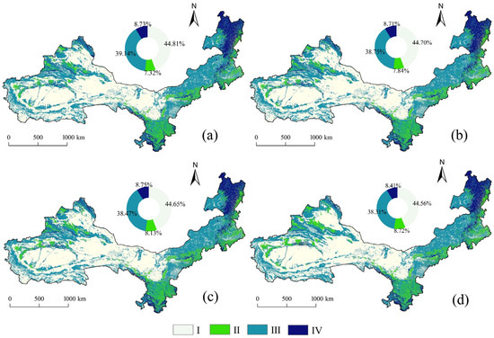
Figure 5.
Spatial and temporal distribution of HQ, 1990–2020 ((a): 1990, (b): 2000, (c): 2010, (d): 2020), Note: HQ I–IV represent I (0–0.3), II (0.3–0.6), III (0.6–0.9), and IV (0.9–1).
3.3. LUCC and HQ Under Future Development Scenarios
3.3.1. Spatial and Temporal Distribution of LUCC Under Future Development Scenarios
The PLUS model was employed in this study to simulate and project land-use patterns in ASAR for 2030 under three distinct scenarios. As illustrated in Figure 6, the natural development scenario reveals notable changes in land-use distribution compared to 2020 baseline conditions. While landscape types maintain relative stability overall, key transformations emerge: Arable land shows a significant reduction of approximately 1.41 × 10⁴ km2 (4.97% decrease), whereas forested land remains largely unchanged. Conversely, we observe expansions in grassland (7.61 × 10³ km2 increase), water bodies (1.51 × 10⁴ km2 increase, predominantly in the Tarim Basin and Tianshan Mountains periphery), and built-up areas (4.13 × 10³ km2 increase). The urban expansion exhibits distinct spatial concentration patterns, particularly evident in northwestern Xinjiang, Ningxia, central Gansu, and select areas of Inner Mongolia. These projected changes highlight the varying pressures on different land-use types under business-as-usual development conditions.
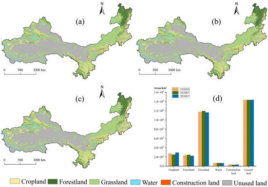
Figure 6.
(a) Natural development scenarios (ND), (b) Ecological protection scenarios (EP), (c) Cropland protection scenarios (CP), (d) Area of land-use types under different scenarios.
3.3.2. Spatial and Temporal Distribution of HQ Under Future Scenarios
Figure 7 presents the projected HQ for 2030 under three distinct scenarios: Natural Development (ND), Ecological Priority (EP), and Cropland Protection (CP). The analysis reveals average HQ values of 0.5215, 0.5264, and 0.5193 for the ND, EP, and CP scenarios, respectively. Notably, the EP scenario demonstrates a 0.94% improvement over ND and a more substantial 1.37% enhancement compared to CP, with Category IV HQ representing the highest proportion at 8.77%. These improvements are primarily attributable to increased woodland area and enhanced vegetation cover under the EP scenario. Spatially, HQ exhibits a pronounced “high-east, low-west” distribution pattern, with optimal values concentrated in northeastern regions. Comparative analysis shows that the EP scenario not only expands high-value areas but also enhances forest cover, thereby contributing significantly to overall HQ improvement. Conversely, the CP scenario results in a 0.42% decline in HQ relative to ND, suggesting that agricultural expansion exerts measurable negative impacts on ecological conditions. These findings underscore the critical role of vegetation conservation in maintaining and improving HQ in ASAR.
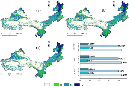
Figure 7.
NHQ in 2030 (a) Distribution of HQ under the ND scenario. (b) Distribution of HQ under the EP scenario. (c) Distribution of HQ under the CP scenario.
3.4. Analysis of the Results of XGBoost-SHAP
3.4.1. Ranking of the Contribution of Different Drivers Based on SHAP
The XGBoost-SHAP analysis in this study reveals distinct temporal patterns in drivers of HQ across ASAR from 1990 to 2020 (Figure 8). The results demonstrate that HQ variations are governed by complex interactions among natural, anthropogenic, and landscape factors, with natural influences consistently dominating. In 1990, climatic factors prevailed, with evapotranspiration (23.67%), distance to water bodies (17.21%), and precipitation (10.27%) emerging as primary determinants. By 2000, a notable shift was observed, with temperature (29.56%) and precipitation (24.86%) becoming most influential, while socioeconomic factors like population density and GDP gained prominence (ranking third and fourth, respectively), signaling increasing anthropogenic pressures.
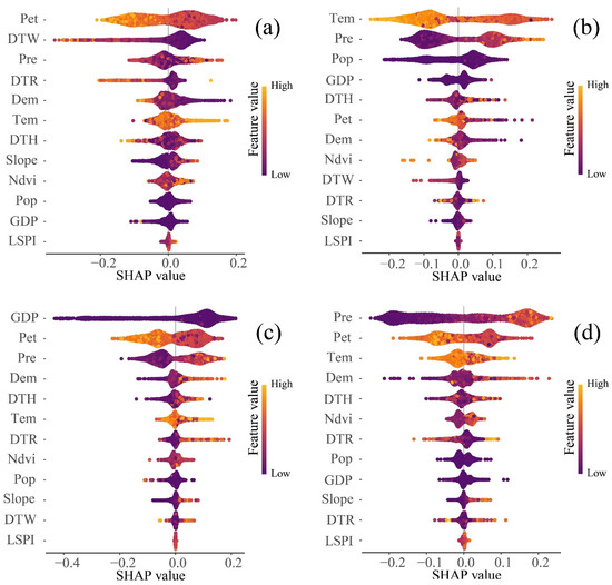
Figure 8.
Summary diagram of SHAP feature analysis ((a–d) represent 1990–2020, respectively).
The 2010 pattern showed GDP rising to dominance (35.14%), surpassing evapotranspiration (18.92%) and precipitation (18.65%), with elevation (DEM, 5.14%) newly emerging as a significant topographic influence. The most recent 2020 data highlight climatic factors’ renewed predominance, where precipitation, evapotranspiration, and temperature collectively accounted for 64.72% of HQ variation. Secondary but notable contributions came from road networks, topographic features, and NDVI, underscoring the multifaceted nature of HQ determinants. These temporal trends reveal an evolving balance between persistent climatic controls and growing human impacts on arid land ecosystems.
3.4.2. Interaction Between Different Driving Factors
The interaction analysis revealed temporal variations in the strength and direction of driving factor interactions, with particularly notable effects among climate-related variables (Figure 9). Throughout the study period, climate factors consistently demonstrated the most significant interactive effects on HQ. In 1990, transportation infrastructure factors (distance to water bodies-DTW, roads-DTR, and highways-DTH) exhibited strong interactions with other variables, while the combination of evapotranspiration and temperature showed predominantly positive effects. By 2000, the interaction between socioeconomic factors (population density ∩ GDP) displayed complex threshold effects, alternating between positive and negative influences. During this period, climate factor interactions became particularly pronounced, with temperature ∩ precipitation combinations exerting primarily positive effects on HQ, while precipitation ∩ evapotranspiration interactions showed more balanced impacts. These climate-driven interaction patterns persisted in 2010, though with more equilibrated directional effects among factors. The most recent 2020 data revealed distinct interaction dynamics, with NDVI ∩ precipitation combinations showing primarily negative effects, contrasting with the more positive interactions observed between NDVI and evapotranspiration. These findings highlight the evolving nature of factor interactions and their complex, sometimes opposing influences on HQ over time.
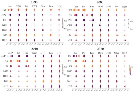
Figure 9.
SHAP interaction diagram between key driving factors.
3.5. Results of GTWR Analysis
The analysis of future scenario impacts in this study reveals significant spatial heterogeneity in how landscape indices influence habitat HQ, as demonstrated by regression coefficients representing effect strength and direction (Figure 10). Due to their limited explanatory power in historical XGBoost modeling, we specifically examined landscape index effects under 2030 scenarios. High-impact zones clustered predominantly in eastern and southwestern Xinjiang, where severe landscape fragmentation degraded ecosystem structure and diminished HQ. Conversely, low-value negative correlation zones coincided with central and eastern regions that maintained superior HQ.
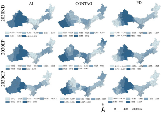
Figure 10.
Spatial and temporal distribution of the regression coefficients of the landscape pattern index in ASAR in 2030 (The magnitude of the regression coefficient represents the extent to which the variable affects HQ, using positive and negative values to distinguish between positive and negative impacts, with positive values indicating positive impacts and negative values indicating negative impacts).
The Aggregation Index (AI) exhibited a distinct west-high, east-low spatial pattern, with western areas showing positive effects that contrasted with central/eastern negative impacts—a consistent pattern across all scenarios. Landscape connectivity (CONTAG) demonstrated uniformly positive HQ relationships throughout western regions, particularly in northeastern/southwestern Xinjiang, with especially strong benefits under the Cropland Protection (CP) scenario in eastern Inner Mongolia, suggesting agricultural conservation may enhance HQ in certain areas. Patch Density (PD) predominantly negatively affected central/eastern regions (typically moderate–high HQ zones), with particularly pronounced detrimental effects in Kashgar’s western periphery under both Natural Development (ND) and Ecological Priority (EP) scenarios compared to CP. These findings collectively highlight how landscape configuration differentially mediates HQ across arid regions, with fragmentation metrics generally exhibiting adverse effects except where connectivity preservation or agricultural management provides compensatory benefits.
4. Discussion
4.1. Impact of Land-Use Change on HQ
Land use/land cover (LULC) patterns serve as fundamental determinants of habitat structure and ecological function in arid and semi-arid ecosystems, where water scarcity imposes critical constraints. The analysis of long-term LULC in this study reveals that approximately 80% of these regions are dominated by unutilized land and grasslands, creating landscapes particularly vulnerable to degradation processes. The spatial distribution of LULC types exhibits strong correlations with HQ, with well-vegetated areas such as the eastern Daxinganling Plain maintaining superior habitat conditions through enhanced microclimate regulation and soil stabilization. Conversely, barren landscapes including the southern Tianshan Mountains and Inner Mongolian Plateau demonstrate severe habitat degradation, manifested through accelerated soil erosion and moisture loss. These natural vulnerabilities are further exacerbated by rapid urbanization, which drives habitat fragmentation through landscape dissection—a phenomenon well-documented in global studies of dryland ecosystems [58,59,60].
The ecological sensitivity of arid systems stems from their characteristic low precipitation and high evapotranspiration rates, making them exceptionally responsive to land-use modifications. The findings indicate that the predominance of unproductive land covers (deserts, bare soils) coupled with limited arable land and water resources (<20% combined coverage) creates fundamental imbalances that accelerate desertification under anthropogenic pressures [61]. Intensive grazing, unsustainable agricultural practices, and vegetation removal collectively degrade soil structure, deplete organic matter, and enhance eolian processes [62]. This degradation cascade reduces ecosystem carrying capacity, ultimately diminishing biodiversity through habitat simplification. Conservation strategies must therefore prioritize sustainable land management approaches, including rotational grazing systems and soil moisture conservation techniques, to mitigate these impacts [63,64]. Future research directions should incorporate advanced remote sensing platforms to better resolve the interacting effects of climate variability and human activities on these fragile ecosystems [65,66,67].
4.2. Analysis of Spatial and Temporal Heterogeneity of HQ and Its Drivers in ASAR
In this study, the XGBoost model alongside the SHAP interpretability framework was employed to analyze the drivers of HQ in ASAR. This integrated approach significantly enhanced both the predictive accuracy and mechanistic interpretability of HQ dynamics. By assigning Shapley values to each feature, the relative contributions of natural and anthropogenic factors to spatial and temporal variations in HQ were quantitatively assessed. The findings reveal that HQ distribution is shaped by a complex interplay of natural factors (e.g., climate, elevation, slope) and anthropogenic influences (e.g., GDP, population density, road proximity), as well as landscape transformations. Overall, both natural and anthropogenic factors exerted negative pressures on HQ, though their relative dominance shifted over time. Among the 12 drivers examined, climatic variables—particularly temperature, precipitation, and evapotranspiration (ET)—emerged as the primary determinants of HQ in 1990. ET plays a critical role in sustaining atmospheric water vapor, especially in densely vegetated areas such as forests, where it reinforces local precipitation through vegetation-precipitation feedback mechanisms [68]. This process ensures freshwater availability, thereby supporting habitat stability. By the 2000s, precipitation and temperature remained pivotal, but road proximity (e.g., distance to railroads [DTR] and water bodies [DTW]) also emerged as significant secondary drivers.
Socioeconomic factors exhibited growing influence over time, reflecting intensified human activity. GDP, a proxy for anthropogenic pressure [69], became the most dominant factor by 2010, underscoring the escalating impact of economic development on habitat degradation. Meanwhile, elevation (DEM) consistently ranked as the fourth-most influential factor across all study years, highlighting its persistent role in mediating habitat suitability. Notably, in 2020, NDVI (Normalized Difference Vegetation Index) rose to the sixth position among drivers, serving as an indirect indicator of environmental conditions. NDVI integrates responses to climatic variables (e.g., precipitation, temperature, soil moisture) and vegetation health, making it a valuable metric for assessing habitat suitability [70]. The interactions between climatic and anthropogenic drivers create heterogeneous spatial patterns of HQ in ASAR. Importantly, the analysis suggests nonlinearities and threshold effects among these factors. Future research should prioritize identifying these critical thresholds (e.g., tipping points in climate or land-use intensity) to quantify how driver impacts shift before and after threshold crossings [71]. Such insights could inform more targeted conservation strategies, ensuring ecosystem resilience under escalating environmental change.
Our finding that natural factors exert the most significant influence on habitat quality (HQ) in the study area (ASAR) aligns with some characteristics of arid and semi-arid ecosystems globally but also reveals distinct particularities when contrasted with representative regional studies [72]. In the Central Asian steppe, a typical arid–semiarid zone, most studies identify socioeconomic factors—especially livestock grazing intensity and agricultural reclamation—as the dominant drivers of HQ degradation. This is attributed to decades of large-scale pastoralism and irrigation agriculture that directly alter grassland and wetland habitats [73]. In China’s Loess Plateau, another ecologically fragile arid-semiarid region, studies consistently highlight the co-dominance of human activities and climatic factors in regulating HQ, reflecting the region’s long history of intensive human intervention [74]. By contrast, the dominance of natural factors in our study area stems from its unique ecological and socioeconomic context: ASAR has relatively sparse population density, limited large-scale agricultural or urban expansion, and native vegetation (e.g., desert steppe, alpine meadow) that is highly sensitive to subtle climatic fluctuations. Precipitation variability directly governs vegetation coverage and productivity—the core determinants of HQ—while temperature regulates the timing of vegetation growth and soil moisture retention [75]. Human activities exert localized impacts but do not override the macro-control of natural factors, which distinguishes ASAR from arid–semiarid regions heavily modified by intensive human exploitation [76]. This contrast underscores that the drivers of HQ in arid and semi-arid zones are not uniform but are shaped by the interplay of local ecological conditions, historical land-use patterns, and socioeconomic intensity. Our results fill a gap in understanding HQ dynamics in “less disturbed” arid-semiarid regions, complementing findings from human-dominated counterparts and providing a more comprehensive framework for global arid zone ecological research.
The spatially heterogeneous effects of the aggregation index on habitat quality (HQ)—manifesting as positive impacts in the west and negative impacts in the east of the study area, as revealed by GTWR results—are rooted in profound differences in environmental backgrounds and human-land interaction patterns between the two regions. In the western part, the landscape is dominated by natural ecosystems such as desert steppes, alpine meadows, and fragmented oases, with sparse population density and limited human disturbance [77]. Here, the aggregation index primarily reflects the connectivity of natural habitat patches: higher aggregation means reduced fragmentation of native vegetation and enhanced ecological processes like species migration and resource circulation, which directly mitigate habitat degradation and improve HQ. For instance, aggregated grassland patches in the west can better retain soil moisture and resist wind erosion, forming stable microhabitats that support higher biodiversity [78]. By contrast, the eastern region has a more intensive human footprint, characterized by concentrated croplands, expanding built-up areas, and fragmented natural habitats [79]. In this context, the aggregation index is largely driven by the clustering of anthropogenic land uses. Such aggregation strengthens the spread of anthropogenic threats—including pesticide use, soil compaction, and habitat conversion—which override the ecological benefits of patch connectivity and exert negative pressure on remaining natural habitats. Additionally, the eastern region’s relatively higher baseline HQ makes it more sensitive to anthropogenic disturbances associated with aggregated land uses, while the west’s lower baseline HQ is more responsive to improvements in natural patch connectivity [80]. This divergence underscores how the same landscape metric can exert contrasting ecological effects depending on the dominant land-use type and disturbance intensity shaped by local environmental and socioeconomic contexts.
4.3. Policy Implications
The present study demonstrates that the spatial heterogeneity of HQ has increased significantly due to the combined effects of landscape pattern evolution, climate change, and intensified human activities. The findings reveal that HQ is markedly higher in regions with greater vegetation cover, underscoring the critical role of land-use type in sustaining ecosystem functions. In recent years, China has prioritized ecological land protection through large-scale initiatives such as the “Three Norths” shelterbelt program and grassland restoration projects. Nevertheless, escalating anthropogenic disturbances in ASAR continue to threaten habitat integrity. Multi-scenario simulations for 2030 yield key insights: HQ under the cropland protection scenario (CP) exhibits a declining trend, whereas the ecological protection scenario (EP) demonstrates a relative advantage, with improvements of 0.94% and 1.37% over other scenarios. These results highlight the delicate trade-off between agricultural production and ecological conservation. Policy formulation should avoid a uniform approach—such as prioritizing high-value habitat areas while restricting development in low-value zones—and instead adopt a more nuanced strategy. This entails systematically evaluating regional landscape patterns and multidimensional drivers of HQ to develop differentiated conservation plans that enhance ecological functionality while preserving natural attributes. A landscape ecology-based governance framework is essential for achieving sustained environmental improvement.
At the policy level, three key recommendations are proposed: First, implement rotational fallow systems and “returning farmland to forests” initiatives, prioritizing the restoration of critical ecosystems (e.g., lakes, wetlands, and forests) while safeguarding arable land limits. Second, establish ecological buffer zones and biological corridors, coupled with zoning controls on development intensity, to mitigate ecological imbalances from excessive land use. Notably, conservation strategies must be regionally tailored; for instance, ecologically vulnerable areas like the Tarim Basin and Junggar Basin periphery require measures focused on reducing landscape fragmentation and maintaining integrity. Third, cross-administrative collaborative mechanisms—including joint monitoring, data sharing, and unified management—should be institutionalized to optimize resource allocation, prevent large-scale ecological risks, and foster synergies among population, societal, and environmental goals [81,82]. Methodologically, the integration of multi-temporal remote sensing data with spatial econometric modeling in this study offers a novel lens for analyzing HQ dynamics. Scenario analyses further illuminate the tension between short-term economic gains and long-term ecological resilience, providing a scientific basis for balanced land-use planning. These contributions not only advance landscape ecology theory but also offer actionable insights for sustainable policy-making in ecologically sensitive regions.
5. Conclusions
This study analyses spatiotemporal land-use changes in ASAR from 1990 to 2020, integrating the PLUS and InVEST models to evaluate historical and future habitat quality (HQ) dynamics. The XGBoost-SHAP and GTWR models were further employed to quantify the impacts of diverse driving factors on HQ. Between 1990 and 2020, cropland and built-up land expanded significantly, while forest and grassland areas declined, with grasslands exhibiting the highest turnover (net transfers exceeding 40% of the total area). Class I habitats dominated the landscape (averaging 43.73% coverage), followed by Class III habitats (38.67%). High-value HQ clusters were predominantly concentrated in the eastern and northeastern study areas, where vegetation cover was denser. Projections under future scenarios revealed that the Ecological Protection (EP) scenario yielded the most substantial HQ improvement, outperforming alternative development pathways.
Natural drivers exerted stronger influences on HQ than socioeconomic factors, with climatic variables showing notable interdependencies and road-related metrics playing a pivotal role via interactions with other drivers. GTWR results highlighted spatial heterogeneity: positive correlations clustered in eastern and southwestern Xinjiang, while negative correlations prevailed in central-eastern zones. These findings underscore the need for spatially tailored strategies—prioritizing fragile areas, designating grassland protection belts, controlling built-up land expansion, and integrating the EP scenario into planning—to balance development and restoration. For policymakers, the measures offer actionable guidelines, and the modeling approach is replicable globally. Future research could incorporate high-resolution climate data and socioeconomic models, or couple with ecosystem service value tools. Domestically, the framework adapts to China’s Loess Plateau and Qinghai–Tibet Plateau; globally, it informs arid-zone management in Central Asia, the Sahara, and the Americas, enabling cross-regional knowledge sharing.
Supplementary Materials
The following supporting information can be downloaded at: https://www.mdpi.com/article/10.3390/land14101937/s1, Figure S1: LSPI for different land use types; Table S1: Threat factor parameter table; Table S2: Threats to habitat sensitivity from different land use types; Table S3: Summary of GTWR model parameters; Table S4: Land-use transfer matrix for Arid and semi-arid regions, 1990–2020; Figure S2: Characteristics of LSPI distribution in Arid and semi-arid regions in 2020; Table S5: Evaluation of the accuracy of XGBoost model.
Author Contributions
S.L.: methodology, software, data curation, writing—original draft; J.H.: conceptualization, funding acquisition. All authors have read and agreed to the published version of the manuscript.
Funding
This research was supported by the Ningxia Business Environment Third-Party Monitoring and Evaluation Project in 2023.
Data Availability Statement
The original contributions presented in this study are included in the article/Supplementary Materials. Further inquiries can be directed to the corresponding author.
Conflicts of Interest
The authors declare no conflicts of interest. The funders had no role in the design of the study; in the collection, analyses, or interpretation of data; in the writing of the manuscript; or in the decision to publish the results.
References
- Costanza, R.; Mageau, M. What Is a Healthy Ecosystem? Aquat. Ecol. 1999, 33, 105–115. [Google Scholar] [CrossRef]
- Daily, G.C.; Matson, P.A. Ecosystem Services: From Theory to Implementation. Proc. Natl. Acad. Sci. USA 2008, 105, 9455–9456. [Google Scholar] [CrossRef]
- Li, Y.; Yang, X.; Qi, H.; Zhang, J.; Shao, J.; Zhou, J.; Zhang, M. Characterization of the Spatial and Temporal Evolution of the Land Use and the Quality of the Habitat in the Region along the Construction Line of the Railway. Ecol. Indic. 2025, 173, 113368. [Google Scholar] [CrossRef]
- Wu, S.; Chen, J.; Jiang, S.; Zhang, R.; Li, Z.; Wang, L.; Li, K. Invasion Risk of Typical Invasive Alien Plants in Mountainous Areas and Their Interrelationship with Habitat Quality: A Case Study of Badong County in Central China. J. Environ. Manag. 2025, 380, 125083. [Google Scholar] [CrossRef] [PubMed]
- Zhao, J.; Yu, L.; Newbold, T.; Chen, X. Trends in Habitat Quality and Habitat Degradation in Terrestrial Protected Areas. Conserv. Biol. 2025, 39, e14348. [Google Scholar] [CrossRef]
- Xia, J.; Ning, L.; Wang, Q.; Chen, J.; Wan, L.; Hong, S. Vulnerability of and Risk to Water Resources in Arid and Semi-Arid Regions of West China under a Scenario of Climate Change. Clim. Change 2017, 144, 549–563. [Google Scholar] [CrossRef]
- Cui, L.; Shi, J. Evaluation and Comparison of Growing Season Metrics in Arid and Semi-Arid Areas of Northern China under Climate Change. Ecol. Indic. 2021, 121, 107055. [Google Scholar] [CrossRef]
- Li, Y.; Liu, W.; Feng, Q.; Zhu, M.; Yang, L.; Zhang, J. Quantitative Assessment for the Spatio-temporal Changes of Ecosystem Services, Tradeoff–Synergy Relationships and Drivers in the Semi-Arid Regions of China. Remote Sens. 2022, 14, 239. [Google Scholar] [CrossRef]
- Pan, N.; Du, Q.; Guan, Q.; Tan, Z.; Sun, Y.; Wang, Q. Ecological Security Assessment and Pattern Construction in Arid and Semi-Arid Areas: A Case Study of the Hexi Region, NW China. Eco-Log. Indic. 2022, 138, 108797. [Google Scholar] [CrossRef]
- Diaz, R.J.; Solan, M.; Valente, R.M. A Review of Approaches for Classifying Benthic Habitats and Evaluating Habitat Quality. J. Environ. Manag. 2004, 73, 165–181. [Google Scholar] [CrossRef]
- Ding, Q.; Chen, Y.; Bu, L.; Ye, Y. Multi-Scenario Analysis of Habitat Quality in the Yellow River Delta by Coupling FLUS with InVEST Model. Int. J. Environ. Res. Public Health 2021, 18, 2389. [Google Scholar] [CrossRef]
- Wang, B.; Cheng, W. Effects of Land Use/Cover on Regional Habitat Quality under Different Geomorphic Types Based on InVEST Model. Remote Sens. 2022, 14, 1279. [Google Scholar] [CrossRef]
- Berta Aneseyee, A.; Noszczyk, T.; Soromessa, T.; Elias, E. The InVEST Habitat Quality Model Associated with Land Use/Cover Changes: A Qualitative Case Study of the Winike Watershed in the Omo-Gibe Basin, Southwest Ethiopia. Remote Sens. 2020, 12, 1103. [Google Scholar] [CrossRef]
- Wang, C.; Wang, Q.; Liu, N.; Sun, Y.; Guo, H.; Song, X. The Impact of LUCC on the Spatial Pattern of Ecological Network during Urbanization: A Case Study of Jinan City. Ecol. Dicators 2023, 155, 111004. [Google Scholar] [CrossRef]
- Zhao, Y.; Kasimu, A.; Gao, P.; Liang, H. Spatiotemporal Changes in The Urban Landscape Pattern and Driving Forces of LUCC Characteristics in The Urban Agglomeration on The Northern Slope of The Tianshan Mountains from 1995 to 2018. Land 2022, 11, 1745. [Google Scholar] [CrossRef]
- Deng, L.; Zhang, Q.; Cheng, Y.; Cao, Q.; Wang, Z.; Wu, Q.; Qiao, J. Underlying the Influencing Factors behind the Heterogeneous Change of Urban Landscape Patterns since 1990: A Multiple Dimension Analysis. Ecol. Indic. 2022, 140, 108967. [Google Scholar] [CrossRef]
- Steinhardt, U.; Volk, M. Meso-Scale Landscape Analysis Based on Landscape Balance Investigations: Problems and Hierarchical Approaches for Their Resolution. Ecol. Model. 2003, 168, 251–265. [Google Scholar] [CrossRef]
- Teng, S.N.; Svenning, J.-C.; Santana, J.; Reino, L.; Abades, S.; Xu, C. Linking Landscape Ecology and Macroecology by Scaling Biodiversity in Space and Time. Curr. Landsc. Ecol. Rep. 2020, 5, 25–34. [Google Scholar] [CrossRef]
- Wu, J.; Luo, J.; Zhang, H.; Qin, S.; Yu, M. Projections of Land Use Change and Habitat Quality Assessment by Coupling Climate Change and Development Patterns. Sci. Total Environ. 2022, 847, 157491. [Google Scholar] [CrossRef]
- Chen, S.; Liu, X. Spatio-Temporal Variations of Habitat Quality and Its Driving Factors in the Yangtze River Delta Region of China. Glob. Ecol. Conserv. 2024, 52, e02978. [Google Scholar] [CrossRef]
- Dong, J.; Zhang, Z.; Liu, B.; Zhang, X.; Zhang, W.; Chen, L. Spatiotemporal Variations and Driving Factors of Habitat Quality in the Loess Hilly Area of the Yellow River Basin: A Case Study of Lanzhou City, China. J. Arid. Land 2022, 14, 637–652. [Google Scholar] [CrossRef]
- Liu, Y.; Wang, Y.; Lin, Y.; Ma, X.; Guo, S.; Ouyang, Q.; Sun, C. Habitat Quality Assessment and Driving Factors Analysis of Guangdong Province, China. Sustainability 2023, 15, 11615. [Google Scholar] [CrossRef]
- Reichstein, M.; Camps-Valls, G.; Stevens, B.; Jung, M.; Denzler, J.; Carvalhais, N. Prabhat Deep Learning and Process Understanding for Data-Driven Earth System Science. Nature 2019, 566, 195–204. [Google Scholar] [CrossRef] [PubMed]
- Cai, A.; Chang, N.; Zhang, W.; Liang, G.; Zhang, X.; Hou, E.; Jiang, L.; Chen, X.; Xu, M.; Luo, Y. The Spatial Patterns of Litter Turnover Time in Chinese Terrestrial Ecosystems. Eur. J. Soil Sci. 2020, 71, 856–867. [Google Scholar] [CrossRef]
- Liu, Y.; Wang, Y.; Zhang, J. New Machine Learning Algorithm: Random Forest. In Information Computing and Applications; Liu, B., Ma, M., Chang, J., Eds.; Springer: Berlin, Heidelberg, 2012; pp. 246–252. [Google Scholar]
- Woo, S.; Kim, W.; Jung, C.; Lee, J.; Kim, Y.; Kim, S. Spatial Analysis of Aquatic Ecological Health under Future Climate Change Using Extreme Gradient Boosting Tree (XGBoost) and SWAT. Water 2024, 16, 2085. [Google Scholar] [CrossRef]
- Zhou, B.; Chen, G.; Yu, H.; Zhao, J.; Yin, Y. Revealing the Nonlinear Impact of Human Activities and Climate Change on Ecosystem Services in the Karst Region of Southeastern Yunnan Using the XGBoost–SHAP Model. Forests 2024, 15, 1420. [Google Scholar] [CrossRef]
- Liu, X.; Liang, X.; Li, X.; Xu, X.; Ou, J.; Chen, Y.; Li, S.; Wang, S.; Pei, F. A Future Land Use Simulation Model (FLUS) for Simulating Multiple Land Use Scenarios by Coupling Human and Natural Effects. Landsc. Urban Plan. 2017, 168, 94–116. [Google Scholar] [CrossRef]
- Dai, L.; Li, S.; Lewis, B.J.; Wu, J.; Yu, D.; Zhou, W.; Zhou, L.; Wu, S. The Influence of Land Use Change on the Spatial–Temporal Variability of Habitat Quality between 1990 and 2010 in Northeast China. J. For. Res. 2019, 30, 2227–2236. [Google Scholar] [CrossRef]
- Xiong, Z.; Yao, S.; Liu, H.; Yu, L. Multi-Scenario Forecasting of Land Use and Ecosystem Service Values in Coastal Regions: A Case Study of the Chaoshan Area, China. ISPRS Int. J. Geo-Inf. 2025, 14, 160. [Google Scholar] [CrossRef]
- Feng, S.; Zhao, W.; Yan, J.; Xia, F.; Pereira, P. Land Degradation Neutrality Assessment and Factors Influencing It in China’s Arid and Semiarid Regions. Sci. Total Environ. 2024, 925, 171735. [Google Scholar] [CrossRef]
- Wang, Q.; Guan, Q.; Sun, Y.; Du, Q.; Xiao, X.; Luo, H.; Zhang, J.; Mi, J. Simulation of Future Land Use/Cover Change (LUCC) in Typical Watersheds of Arid Regions under Multiple Scenarios. J. Environ. Manag. 2023, 335, 117543. [Google Scholar] [CrossRef]
- Liu, K.; Wu, B.; Gao, F.; Chen, Y.; He, B.; Waheed, A.; Aili, A.; Xu, Z.; Han, F.; Xu, H. Dynamic Simulation and Key Influencing Factors of Carbon Storage in the Water-Depleted Zones of an Arid Inland River Basin: Insights from the Tarim River Mainstream. Ecol. Inform. 2025, 90, 103286. [Google Scholar] [CrossRef]
- Gomes, E.; Inácio, M.; Bogdzevič, K.; Kalinauskas, M.; Karnauskaitė, D.; Pereira, P. Future Scenarios Impact on Land Use Change and Habitat Quality in Lithuania. Environ. Res. 2021, 197, 111101. [Google Scholar] [CrossRef] [PubMed]
- Deng, G.; Jiang, H.; Ma, S.; He, C.; Sheng, L.; Wen, Y. Revealing the Impacts of Different Urban Development on Habitat Quality: A Case Study of the Changchun–Jilin Region of China. J. Clean. Prod. 2025, 511, 145661. [Google Scholar] [CrossRef]
- Yang, D.; Liu, W.; Tang, L.; Chen, L.; Li, X.; Xu, X. Estimation of Water Provision Service for Monsoon Catchments of South China: Applicability of the InVEST Model. Landsc. Urban Plan. 2019, 182, 133–143. [Google Scholar] [CrossRef]
- Hou, Y.; Lü, Y.; Chen, W.; Fu, B. Temporal Variation and Spatial Scale Dependency of Ecosystem Service Interactions: A Case Study on the Central Loess Plateau of China. Landsc. Ecol. 2017, 32, 1201–1217. [Google Scholar] [CrossRef]
- Nelson, E.; Mendoza, G.; Regetz, J.; Polasky, S.; Tallis, H.; Cameron, D.; Chan, K.M.; Daily, G.C.; Goldstein, J.; Kareiva, P.M.; et al. Modeling Multiple Ecosystem Services, Biodiversity Conservation, Commodity Production, and Tradeoffs at Landscape Scales. Front. Ecol. Environ. 2009, 7, 4–11. [Google Scholar] [CrossRef]
- Sharma, R.; Nehren, U.; Rahman, S.A.; Meyer, M.; Rimal, B.; Aria Seta, G.; Baral, H. Modeling Land Use and Land Cover Changes and Their Effects on Biodiversity in Central Kalimantan, Indonesia. Land 2018, 7, 57. [Google Scholar] [CrossRef]
- Su, J.; Zhang, R.; Wu, M.; Yang, R.; Liu, Z.; Xu, X. Correlation between Spatial-Temporal Changes in Landscape Patterns and Habitat Quality in the Yongding River Floodplain, China. Land 2023, 12, 807. [Google Scholar] [CrossRef]
- Xiang, Q.; Kan, A.; Yu, X.; Liu, F.; Huang, H.; Li, W.; Gao, R. Assessment of Topographic Effect on Habitat Quality in Mountainous Area Using InVEST Model. Land 2023, 12, 186. [Google Scholar] [CrossRef]
- Schooley, R.L.; Branch, L.C. Habitat Quality of Source Patches and Connectivity in Fragmented Landscapes. Biodivers. Conserv. 2011, 20, 1611–1623. [Google Scholar] [CrossRef]
- Zhu, Y.; Yan, L.; Wang, Y.; Zhang, J.; Liang, L.; Xu, Z.; Guo, J.; Yang, R. Landscape Pattern Change and Its Correlation with Influencing Factors in Semiarid Areas, Northwestern China. Chemosphere 2022, 307, 135837. [Google Scholar] [CrossRef]
- Chen, C.; Zhang, X.; Hu, J.; Hu, B.; Yuan, J.; Xing, Y.; Zhou, D. Landscape Dynamics Driven by Socioeconomic Factors of the Coastal Cities along the Yellow Sea and Bohai Sea over the Last 40 Years. Ecol. Indic. 2025, 179, 114156. [Google Scholar] [CrossRef]
- Zhang, F.; Yushanjiang, A.; Wang, D. Ecological Risk Assessment Due to Land Use/Cover Changes (LUCC) in Jinghe County, Xinjiang, China from 1990 to 2014 Based on Landscape Patterns and Spatial Statistics. Environ. Earth Sci. 2018, 77, 491. [Google Scholar] [CrossRef]
- Pu, J.; Shen, A.; Liu, C.; Wen, B. Impacts of Ecological Land Fragmentation on Habitat Quality in the Taihu Lake Basin in Jiangsu Province, China. Ecol. Indic. 2024, 158, 111611. [Google Scholar] [CrossRef]
- Wang, S.Q.; Zheng, X.Q.; Zang, X.B. Accuracy Assessments of Land Use Change Simulation Based on Markov-Cellular Automata Model. Procedia Environ. Sci. 2012, 13, 1238–1245. [Google Scholar] [CrossRef]
- Liang, X.; Guan, Q.; Clarke, K.C.; Liu, S.; Wang, B.; Yao, Y. Understanding the Drivers of Sustainable Land Expansion Using a Patch-Generating Land Use Simulation (PLUS) Model: A Case Study in Wuhan, China. Comput. Environ. Urban Syst. 2021, 85, 101569. [Google Scholar] [CrossRef]
- Zhao, X.; Wang, P.; Gao, S.; Yasir, M.; Islam, Q.U. Combining LSTM and PLUS Models to Predict Future Urban Land Use and Land Cover Change: A Case in Dongying City, China. Remote Sens. 2023, 15, 2370. [Google Scholar] [CrossRef]
- Duan, Y.; Halike, A.; Luo, J.; Yao, K.; Yao, L.; Tang, H.; Tuheti, B. Multi-Scale Supply and Demand Relationships of Ecosystem Services Under Multiple Scenarios and Ecological Zoning to Promote Sustainable Urban Ecological Development in Arid Regions of China. Sustainability 2024, 16, 9641. [Google Scholar] [CrossRef]
- Song, J.; He, X.; Zhang, F.; Ma, X.; Jim, C.Y.; Johnson, B.A.; Chan, N.W. Analyzing and Pre-dicting LUCC and Carbon Storage Changes in Xinjiang’s Arid Ecosystems Under the Carbon Neutrality Goal. Remote Sens. 2024, 16, 4439. [Google Scholar] [CrossRef]
- Kruk, M. SHAP-NET, a Network Based on Shapley Values as a New Tool to Improve the Ex-plainability of the XGBoost-SHAP Model for the Problem of Water Quality. Environ. Model. Softw. 2025, 188, 106403. [Google Scholar] [CrossRef]
- Sun, D.; Wu, X.; Wen, H.; Ma, X.; Zhang, F.; Ji, Q.; Zhang, J. Ecological Security Pattern Based on XGBoost-MCR Model: A Case Study of the Three Gorges Reservoir Region. J. Clean. Prod. 2024, 470, 143252. [Google Scholar] [CrossRef]
- Wen, H.; Liu, B.; Di, M.; Li, J.; Zhou, X. A SHAP-Enhanced XGBoost Model for Interpretable Prediction of Coseismic Landslides. Adv. Space Res. 2024, 74, 3826–3854. [Google Scholar] [CrossRef]
- Zhang, H.; Fu, J.; Li, F.; Chen, Q.; Ye, T.; Zhang, Y.; Yang, X. Fine-Scale Population Mapping on Tibetan Plateau Using the Ensemble Machine Learning Methods and Multisource Data. Ecol. Indic. 2024, 166, 112307. [Google Scholar] [CrossRef]
- Tian, Y.; Zhang, Q.; Tao, J.; Zhang, Y.; Lin, J.; Bai, X. Use of Interpretable Machine Learning for Understanding Ecosystem Service Trade-Offs and Their Driving Mechanisms in Karst Peak-Cluster Depression Basin, China. Ecol. Indic. 2024, 166, 112474. [Google Scholar] [CrossRef]
- Hu, J.; Zhang, J.; Li, Y. Exploring the Spatial and Temporal Driving Mechanisms of Landscape Patterns on Habitat Quality in a City Undergoing Rapid Urbanization Based on GTWR and MGWR: The Case of Nanjing, China. Ecol. Indic. 2022, 143, 109333. [Google Scholar] [CrossRef]
- He, J.; Huang, J.; Li, C. The Evaluation for the Impact of Land Use Change on Habitat Quality: A Joint Contribution of Cellular Automata Scenario Simulation and Habitat Quality Assessment Model. Ecol. Model. 2017, 366, 58–67. [Google Scholar] [CrossRef]
- Liang, Y.; Liu, L. Simulating Land-Use Change and Its Effect on Biodiversity Conservation in a Watershed in Northwest China. Ecosyst. Health Sustain. 2017, 3, 1335933. [Google Scholar] [CrossRef]
- Liu, Y.; Huang, X.; Yang, H.; Zhong, T. Environmental Effects of Land-Use/Cover Change Caused by Urbanization and Policies in Southwest China Karst Area–A Case Study of Guiyang. Habitat Int. 2014, 44, 339–348. [Google Scholar] [CrossRef]
- Jiang, P.; Cheng, L.; Li, M.; Zhao, R.; Duan, Y. Impacts of LUCC on Soil Properties in the Ri-parian Zones of Desert Oasis with Remote Sensing Data: A Case Study of the Middle Heihe River Basin, China. Sci. Total Environ. 2015, 506, 259–271. [Google Scholar] [CrossRef]
- Li, Q.; Sun, Y.; Yuan, W.; Lyu, S.; Wan, F. Streamflow Responses to Climate Change and LUCC in a Semi-Arid Watershed of Chinese Loess Plateau. J. Arid. Land 2017, 9, 609–621. [Google Scholar] [CrossRef][Green Version]
- Yang, Y.; Xie, J.; Sheng, H.; Chen, G.; Li, X.; Yang, Z. The Impact of Land Use/Cover Change on Storage and Quality of Soil Organic Carbon in Midsubtropical Mountainous Area of Southern China. J. Geogr. Sci. 2009, 19, 49–57. [Google Scholar] [CrossRef]
- Yang, Q.; Huang, X.; Li, J. Assessing the Relationship between Surface Urban Heat Islands and Landscape Patterns across Climatic Zones in China. Sci. Rep. 2017, 7, 9337. [Google Scholar] [CrossRef] [PubMed]
- He, C.; Liu, Z.; Tian, J.; Ma, Q. Urban Expansion Dynamics and Natural Habitat Loss in China: A Multiscale Landscape Perspective. Glob. Change Biol. 2014, 20, 2886–2902. [Google Scholar] [CrossRef]
- Hodgson, J.A.; Moilanen, A.; Wintle, B.A.; Thomas, C.D. Habitat Area, Quality and Connectivity: Striking the Balance for Efficient Conservation. J. Appl. Ecol. 2011, 48, 148–152. [Google Scholar] [CrossRef]
- Ke, X.; van Vliet, J.; Zhou, T.; Verburg, P.H.; Zheng, W.; Liu, X. Direct and Indirect Loss of Natural Habitat Due to Built-up Area Expansion: A Model-Based Analysis for the City of Wuhan, China. Land Use Policy 2018, 74, 231–239. [Google Scholar] [CrossRef]
- Kirschbaum, M.U.F.; Saggar, S.; Tate, K.R.; Giltrap, D.L.; Ausseil, A.-G.E.; Greenhalgh, S.; Whitehead, D. Comprehensive Evaluation of the Climate-Change Implications of Shifting Land Use between Forest and Grassland: New Zealand as a Case Study. Agric. Ecosyst. Environ. 2012, 150, 123–138. [Google Scholar] [CrossRef]
- Gosselin, F.; Callois, J.-M. Relationships between Human Activity and Biodiversity in Europe at the National Scale: Spatial Density of Human Activity as a Core Driver of Biodiversity Erosion. Ecol. Indic. 2018, 90, 356–365. [Google Scholar] [CrossRef]
- Weber, D.; Schaepman-Strub, G.; Ecker, K. Predicting Habitat Quality of Protected Dry Grass-lands Using Landsat NDVI Phenology. Ecol. Indic. 2018, 91, 447–460. [Google Scholar] [CrossRef]
- Zhang, J.; Mengting, L.; Hui, Y.; Xiyun, C.; Chong, F. Critical Thresholds in Ecological Resto-ration to Achieve Optimal Ecosystem Services: An Analysis Based on Forest Ecosystem Restora-tion Projects in China. Land Use Policy 2018, 76, 675–678. [Google Scholar] [CrossRef]
- Cui, L.; Zheng, S.; Jin, Y.; Shen, Z.; Dong, X.; Xu, M. Understanding the Nonlinear Trade-off Relationship to Optimize Urban-Rural Ecosystem Services: A Case Study in Arid and Semi-Arid Region, China. Habitat Int. 2025, 166, 103567. [Google Scholar] [CrossRef]
- Li, J.; Zhao, W.; Ma, X.; Luo, G.; Pereira, P. Ecosystem Service Tradeoff and Synergy Mecha-nisms in the Central Asian Terminal Lake Basin Based on Bayesian Networks. Ecosyst. Serv. 2025, 75, 101768. [Google Scholar] [CrossRef]
- Zhang, Z.; Pan, H.; Liu, Y.; Sheng, S. Ecosystem Services’ Response to Land Use Intensity: A Case Study of the Hilly and Gully Region in China’s Loess Plateau. Land 2024, 13, 2039. [Google Scholar] [CrossRef]
- Yu, H.; Liang, Z.; Zhang, R.; Jia, M.; Li, S.; Li, X.; Li, H. Spatiotemporal Dynamics of Habitat Quality in Semi-Arid Regions: A Case Study of the West Songnen Plain, China. Remote Sens. 2025, 17, 1663. [Google Scholar] [CrossRef]
- Ma, T.; Cheng, W.; Yao, W. Spatiotemporal Evolution and Multi-Scenario Simulation of the Land-Use Cover Change and Habitat Quality in Arid and Semi-Arid Areas: A Case Study of the Urban Agglomeration along the Yellow River in Ningxia, China. Front. Environ. Sci. 2025, 13, 9302. [Google Scholar] [CrossRef]
- Wang, L.; Liu, W.; Feng, Q.; Yin, Z.; Zhu, R.; Zhu, M.; Zhang, J.; Xue, Y.; Chen, Z.; Li, X. Patterns and Drivers of Water-Land Resources Nexus in Arid Inland River Basins of Northwestern China. Environ. Sustain. Indic. 2025, 26, 100702. [Google Scholar] [CrossRef]
- Wu, C.; Gao, P.; Xu, R.; Mu, X.; Sun, W. Influence of Landscape Pattern Changes on Water Conservation Capacity: A Case Study in an Arid/Semiarid Region of China. Ecol. Indic. 2024, 163, 112082. [Google Scholar] [CrossRef]
- Guo, J.; Shen, B.; Li, H.; Wang, Y.; Tuvshintogtokh, I.; Niu, J.; Potter, M.A.; Li, F.Y. Past Dynamics and Future Prediction of the Impacts of Land Use Cover Change and Climate Change on Landscape Ecological Risk across the Mongolian Plateau. J. Environ. Manag. 2024, 355, 120365. [Google Scholar] [CrossRef] [PubMed]
- He, X.; Zhang, F.; Zhou, T.; Xu, Y.; Xu, Y.; Jim, C.Y.; Johnson, B.A.; Ma, X. Human Activities Dominated Terrestrial Productivity Increase over the Past 22 Years in Typical Arid and Semiarid Regions of Xinjiang, China. Catena 2025, 250, 108754. [Google Scholar] [CrossRef]
- Bustamante, M.; Robledo-Abad, C.; Harper, R.; Mbow, C.; Ravindranat, N.H.; Sperling, F.; Haberl, H.; de Pinto, S.A.; Smith, P. Co-Benefits, Trade-Offs, Barriers and Policies for Green-house Gas Mitigation in the Agriculture, Forestry and Other Land Use (AFOLU) Sector. Glob. Change Biol. 2014, 20, 3270–3290. [Google Scholar] [CrossRef]
- Kloffel, T.; Young, E.H.; Borchard, N.; Vallotton, J.D.; Nurmi, E.; Shurpali, N.J.; Tenorio, F.U.; Liu, X.; Young, G.H.F.; Unc, A. The Challenges Fraught Opportunity of Agriculture Expansion into Boreal and Arctic Regions. Agric. Syst. 2022, 203, 103507. [Google Scholar] [CrossRef]
Disclaimer/Publisher’s Note: The statements, opinions and data contained in all publications are solely those of the individual author(s) and contributor(s) and not of MDPI and/or the editor(s). MDPI and/or the editor(s) disclaim responsibility for any injury to people or property resulting from any ideas, methods, instructions or products referred to in the content. |
© 2025 by the authors. Licensee MDPI, Basel, Switzerland. This article is an open access article distributed under the terms and conditions of the Creative Commons Attribution (CC BY) license (https://creativecommons.org/licenses/by/4.0/).