Abstract
Land use/land cover changes (LUCCs) significantly reshape ecosystem services (ESs) within the framework of climate change. Studying LUCC and its impact on ESs is crucial for a comprehensive understanding of the impact of human activities on ecosystems. The InVEST model coupled with the predicted land use data were used to analyze the spatiotemporal characteristics of four ESs (soil conservation (SC), water yield (WY), carbon storage (CS), and habitat quality (HQ)) under three scenarios from 2040 to 2100 and quantified trade-offs/synergies and bundles of these ESs within the Bailong River Basin (BRB). The results indicated that (1) under the SSP1-2.6 scenario, there is an anticipated increase in forestland, a concurrent decrease in grassland, farmland, and built-up land, and an enhancement in four ESs from 2040 to 2100. The forestland and farmland in the SSP2-4.5 scenario showed a gradual decrease, with an expansion of grassland and built-up land. Except for HQ, the other three ESs were reduced. Both forestland and grassland decreased. Built-up land and farmland increased, and ESs decreased significantly under the SSP5-8.5 scenario. (2) Synergistic effects were identified among the ESs, with the most pronounced synergy observed between CS and HQ. Spatially, six pairs of ESs under the SSP1-2.6 scenario showed synergistic effects. Under the SSP2-4.5 and SSP5-8.5 scenarios, most of the ESs present trade-off effects. (3) The characterization of ES bundles revealed that the balanced enhancement of the four ESs predominantly occurred in the southern region of the basin. Among the scenarios, SSP1-2.6 had the highest representation, followed by the SSP2-4.5, while the SSP5-8.5 had the lowest proportion. The findings facilitate the sustainable and balanced development of diverse ESs and offer theoretical and technical insights for devising spatial regulation policies and ecosystem-based management strategies.
1. Introduction
The ES framework acts as an essential bridge between ecosystems and socioeconomic systems, playing a critical role in safeguarding human well-being [1,2]. In the last century, factors such as global climate change [3], environmental pollution [4], ecological destruction [5], resource depletion [6], and LUCC [7] have profoundly affected ecosystem functioning, resulting in considerable modifications to ESs. According to the MEA report, over 60% of the world’s ecosystems are either degrading or have already degraded. The ensuing degradation poses a significant threat to the integrity of regional ecosystems and jeopardizes the feasibility of sustainable socioeconomic development [8,9]. This includes a decline in vegetation productivity, habitat fragmentation, water scarcity [10], and soil and water erosion [11]. Therefore, assessing and identifying the spatial patterns of ESs can offer significant support for their management and inform decision-making processes, thereby helping to mitigate the adverse effects of the threats to these services [12].
In recent years, progress in technologies has catalyzed a significant shift toward quantitative approaches in ecological and environmental studies [13,14]. The availability of diverse datasets, enabled by advanced technologies, lays a solid groundwork for the quantitative assessment of ESs [15,16]. Additionally, the evolution of diverse evaluation techniques has empowered the scientific community to harness existing knowledge for assessing ESs across a range of spatial scales and within multiple planning sectors [17]. The InVEST model, celebrated for its sophisticated capabilities, is particularly adept at visualizing and quantifying [18]. Arunyawat et al. (2016) analyzed the impact of LUCC on ESs based on the InVEST model. Utilizing this tool, they were able to map and quantify various ES functions in Northern Thailand, including SC, WY, CS, and HQ [19]. Yang et al. (2021) applied the InVEST model to assess HQ and analyzed the effects of LUCC on HQ in the Taihang Mountains [20]. Additionally, Li et al. (2021) employed the InVEST model to assess WY in the Danjiang River Basin, thereby assessing the basin’s capacity for water conservation [21]. In a subsequent study, Yang et al. (2023) used the InVEST model to analyze the impact of ecological restoration projects in the Yellow River Delta on changes in HQ and CS [22]. Huang et al. (2024) leveraged the InVEST model to project the spatiotemporal dynamics of WY, HQ, and SC within oases and urban clusters in Xinjiang, China [23]. The InVEST model has been widely recognized for evaluating WY, CS, HQ, and SC. Water resources, being a critical component, are essential in the mitigation of water scarcity and pollution, as well as in maintaining the vitality of aquatic ecosystems. SC is vital for preserving land productivity and fertility, preventing erosion and desertification, and maintaining the balance of soil and water, as well as the surface hydrological cycle. HQ contributes to the healthy development of the ecosystem environment. CS plays an important role in mitigating climate change and protecting biodiversity. These ESs form the foundation of environmental sustainability and societal well-being [24]. Therefore, we quantitatively evaluated the four key ESs (WY, SC, HQ, and CS) of BRB using the InVEST model.
Human activities are a major cause of ecosystem degradation. Among the myriad factors that influence ESs, LUCC emerges as the most dynamic and dominant, with the power to directly alter ecosystems, thereby affecting the sustainability and change in ESs [25,26]. Therefore, the potential negative impact of LUCC on ESs has attracted considerable attention [27,28]. Research does indicate that LUCC is affected by climate change and socioeconomic development [29,30]. The most recent CMIP6 offers a comprehensive framework for exploring various future development scenarios. This is achieved by integrating shared socioeconomic pathways (SSPs) with representative concentration pathways (RCPs) [2,31]. An escalating trend in research is adopting SSP-RCP scenarios to foresee shifts in future land use requirements. In a prominent study, Dong et al. (2018) employed the GCAM to project future land use demands across China and to simulate the spatial distribution of these demands [32]. Recently, many new perspectives have emerged to evaluate the spatiotemporal changes of ESs in SSP-RCP scenarios. Qiu et al. (2023) analyzed the spatiotemporal distribution of LUCC and ESs in Central Asia under different SSP-RCP scenarios using the LUH2 dataset [33]. Guo et al. (2024) [34] and Li et al. (2023) [35] assessed CS in SSP-RCP scenarios using LUH2 data Nonetheless, the majority of these investigations concentrate on LUCC at the national or global scales. In addition, some scholars have predicted the ecosystem of Shenzhen in 2030 based on LUCC [36]. Wu et al. (2022) utilized the FLUS model to assess HQ, integrating a framework that considers climate change and development patterns [37].
However, the existing body of research has predominantly concentrated on the alterations in ESs as a result of LUCC under projected future climate scenarios. However, future changes in multiple ecological services under different LUCCs and climate scenarios, especially in ecologically fragile areas in China, are still unknown. Moreover, assessing ESs in isolation across various scenarios is insufficient to offer tangible directives for environmental management. It is imperative to integrate the interrelationships among ESs into spatial planning and to bolster the nexus between ESs and ecological governance [38]. ESs are not discrete entities. Rather, they are interconnected, with alterations in one ES potentially diminishing or augmenting the capacity of another [39,40]. These interlinkages are characterized as trade-offs and synergies [41]. Scholars acknowledge the significance of ecosystem interdependencies, with extensive research dedicated to their quantitative assessment [42]. However, integrating this analysis into land use planning poses an ongoing challenge. Neglecting the interconnectivity of ESs can impede the enhancement of ecological benefits and may lead to the degradation of ecosystems within land use practices [43,44]. Therefore, clarifying the complex relationships between ecosystems under the background of land use change can promote the healthy development of ecosystems.
To address the above limitations, this research opts for the BRB as the focal study area. The BRB is a pivotal region for water conservation and acts as an essential ecological barrier, with significant water conservation services and high HQ. The basin features highly varied terrain, severe soil erosion, and improvements in SC services that contribute to the ecological security and stability of the watershed. However, the basin is characterized by rugged mountains, deep valleys, and limited land resources. Land reclamation and policy implementations, such as the “grain for green”, may also affect changes in ESs and their interrelationships under the broader context of regional climate change. To this end, considering the ecological and environmental attributes of the research area, as well as the features of the InVEST model, four typical services, namely CS, SC, WY, and HQ, were selected for in-depth analysis. The ES functions under future land use scenarios in the BRB were assessed, and their trade-offs/synergies and bundling were discussed, providing scientific support for regional environmental management, decision-making, and sustainable development. Section 2 offers a detailed description of the study area, the data and their sources, the method used for land use simulation, the method for assessing ESs, and the methods for analyzing ES trade-offs/synergies and identifying ES bundles. Section 3 presents the research findings. Section 4 provides a discussion on the contributions, policy implications, research limitations, and future prospects. Section 5 summarizes the key conclusions. Our objectives are 1) to forecast the forthcoming LUCC trajectories in the BRB from 2040 to 2100; 2) to evaluate the variations in ESs across diverse scenarios; 3) to assess the interplay among ecosystems within the context of various scenarios; 4) to identify ES bundles and provide relevant recommendations for ES management.
2. Materials and Methods
2.1. Study Area
The BRB, defined by the geographic coordinates 32°36′ N to 34°24′ N and 103°00′ E to 105°30′ E, covers an area of 17,756 km2. The BRB primarily encompasses Diebu County, Zhouqu County, Wen County, Tanchang County, and Wudu District (Figure 1). The basin’s topography is marked by elevated terrain in the northwest and lower elevations in the southeast, ranging in altitude from 602 to 5280 m. The predominant landform types within the basin include plateau mountains, river valleys, and loess landforms. There is an obvious vertical change trend in the domain. The valley is warm and rainless, and the high mountain area is cold and rainy. Due to the influence of tectonic movement, regional stratum characteristics, and climate, the soil layer in the watershed is shallow, the site conditions are poor, and the water and soil losses on both sides of the river are serious [45]. With the development of the regional society and economy, forestry resources have been developed and utilized in large quantities in basins, grasslands have been overgrazed, and the regional ecological environment has been seriously degraded.
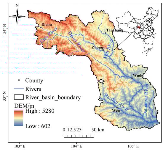
Figure 1.
Location map of the BRB.
2.2. Data Source and Pre-Processing
This study collected multisource datasets to accommodate the diverse data demands of various models, encompassing spreadsheet data, vector data, and raster data across a spectrum of spatial and temporal resolutions. (Table 1). To address the discrepancies in land use data classifications between the two surveys, we performed a reclassification of the datasets from both periods to align their categorizations. All the data underwent format conversion, clipping, projection, and resampling using Python. The sub-basins were delineated using DEM data with the ArcSWAT hydrological analysis tool (Figure 2).

Table 1.
Overview of the Key Datasets.
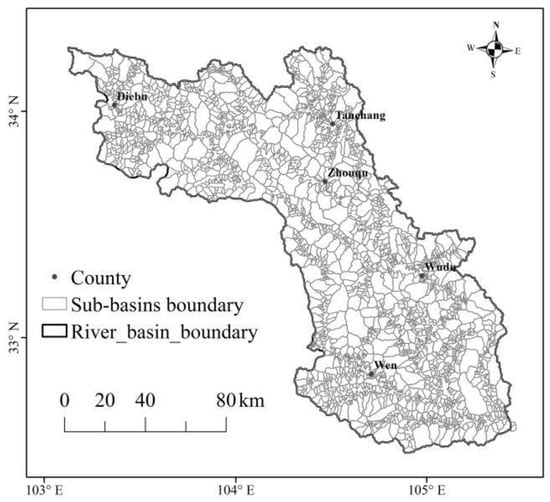
Figure 2.
The boundary of the 1986 sub-basins.
2.3. Method
Our research framework is shown in Figure 3. Initially, based on socioeconomic and climate change data in the SSP-RCP scenario, the PLUS model was used to predict land use from 2040 to 2100. Next, the InVEST model is employed to calculate four types of ESs using land use and climate data. Then, the spatiotemporal distribution characteristics of ES trade-offs/synergies from 2040 to 2100 were revealed. Finally, the SOM method was used to determine the ES bundles. The findings offer significant guidance for ecosystem management and the formulation of implementation plans.
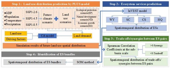
Figure 3.
The research framework.
2.3.1. Simulation of Future Land Use
PLUS Model
We used the PLUS model to simulate land use in the BRB. The PLUS model is a patch-based land use change simulation model [46]. Liang et al. (2022) explained the basic principles and formulas of the PLUS model [46].
Model Validation
Land use is categorized into six types, namely farmland, forestland, grassland, water bodies, built-up land, and unused land, along with 13 subcategories in the BRB. Nineteen driving factors influencing land use change were selected, including socioeconomic, DEM, transportation, and environmental factors. Subsequently, based on the land use data from 2010, a simulation of the land use pattern in 2020 was conducted using transition matrices, domain weights, and land demand. Then, the Kappa statistical method was used to validate the simulation results:
where denotes the proportion of correct simulations, denotes the correct proportion of the model under random conditions, and denotes the proportion of correct simulations under ideal classification conditions. The verification results indicate that the Kappa coefficient is 0.8881. Consequently, the simulation results are deemed reliable and can be utilized for land use projections in the years 2040, 2060, 2080, and 2100 [47,48].
Multi-Scenario Setting
We identified three representative SSP-RCP scenarios within the CMIP6 framework and integrated them with plausible future developmental trajectories to formulate three distinct scenarios: (1) SSP1-2.6 and the ecological protection scenario (SSP126-EP), where ecological conservation is paramount, with socioeconomic development predicated on ecological preservation, a reduction in fossil fuel usage, and the attainment of sustainable green growth; (2) SSP2-4.5 and natural development scenario (SSP245-ND), based on the original land use development evolution; and (3) SSP5-8.5 and economic growth scenario (SSP585-EG), which is dominated by economic development and has the main goals of putting a large amount of fossil fuels into use and economic improvement. We used four driving factors (GDP, POP, temperature, and precipitation) to estimate LUCC under the SSP-RCP scenario [49].
2.3.2. ESs Assessment
SC
SC is calculated through the sediment delivery ratio module in the InVEST model [50]. The specific calculation of the model is as follows:
SEDRET denotes the amount of soil conservation. PKLS denotes the potential soil erosion amount in tons (t). USLE denotes the actual soil erosion amount in tons (t). LS denotes the slope length and slope factor. R and K represent the precipitation and soil erosion factors, respectively. The magnitudes of the C and P factors are between 0 and 1, and the values are assigned by consulting the relevant literature in similar research areas and combining the special conditions of the research area [38] (Table 2).
Table 2.
C and P values for different land use types.
WY
We employed the InVEST model to calculate WY. The calculation formula within the model is presented below:
Y(x) denotes the water production (mm). AET(x) represents the actual evapotranspiration. PET(x) represents the potential evapotranspiration. P(x) denotes the average monthly precipitation. ω(x) is the physical parameters of natural climate and soil properties. AWC(x) represents derived from the plant-available water capacity (PAWC), the maximum rooting depth of the soil, and the minimum value of the vegetation root depth. The Z value ranges from 1 to 10 and denotes the distribution of precipitation in the watershed, as well as other hydrological and geological characteristics, without any units.
Specifically, Sand%, Silt%, Clay%, and C% represent the respective percentage compositions of sand, silt, clay, and organic matter in the soil.
CS
This study used the InVEST model to calculate CS. The calculation formula is:
Cabove denotes the aboveground biomass carbon storage in tons (t). Cbelow signifies the underground biomass carbon storage in tons (t). Csoil represents the soil organic carbon storage in tons (t). Cdead indicates the carbon storage from dead organic matter in tons (t). C is regional carbon storage (t). The carbon density data come from the collection and arrangement of the results, such as [51] and the reference database [52].
HQ
The InVEST model assesses the status of biodiversity through the magnitude of HQ. The calculation formula is:
In the formula, Qxj is the HQ (dimensionless) of grid unit x in land type j; Hj denotes the habitat attribute or suitability of land type j; Dxj signifies the degree of habitat degradation for grid unit x in land type j; k is the half-saturation coefficient; and z is the default normalization constant of the model (z = 2.5).
where is the weight of each threat factor, is the intensity of the threat factor, is the anti-interference level of the habitat, and is the relative sensitivity of different habitats to different threat factors. The habitat degradation degree ranges from 0 to 1, with values close to 1 indicating a high habitat degradation degree [53]. The parameters are detailed in Table 3 and Table 4.
Table 3.
Parameters of threat factors.
Table 4.
Sensitivity parameters of various land types to habitat threat factors.
2.3.3. Trade-Offs/Synergies
This article uses a Spearman correlation analysis method to determine the trade-offs/synergies between ESs. The negative correlation between the ESs represents a trade-off, while the positive correlation represents a synergistic effect. We conducted a Spearman correlation analysis using R 4.4.1 software for the period from 2040 to 2100.
2.3.4. Identification of Bundle
“Bundle” refers to the spatially recurrent aggregation of ESs [54], which can identify various patterns of ES aggregation. We implemented self-organizing maps (SOM) to determine ES bundles at the sub-basin scale. This method assigns each sub-basin to an ES bundle based on the spatial similarity of the four ESs.
3. Results
3.1. LUCC Characteristics in the BRB from 2040 to 2100
Our predicted land use in the BRB from 2040 to 2100 is shown in Figure 4, Figure 5 and Figure 6. From 2040 to 2100, the proportion of forest land will always be the largest (>60%), mainly distributed in the western and southern regions of the basin, with the widest distribution in Diebu County. Grassland (accounting for 12.39% and 17.81% respectively) was distributed on the slopes on both sides of the ravine. Both farmland and built-up land (including industrial land, common land, urban land, village land, township land, and traffic land) are concentrated in flat areas on both sides of the Bailong River and its secondary tributaries. It is worth noting that Wudu District has the largest built-up land area, while Tunchang County has the widest distribution of farmland.
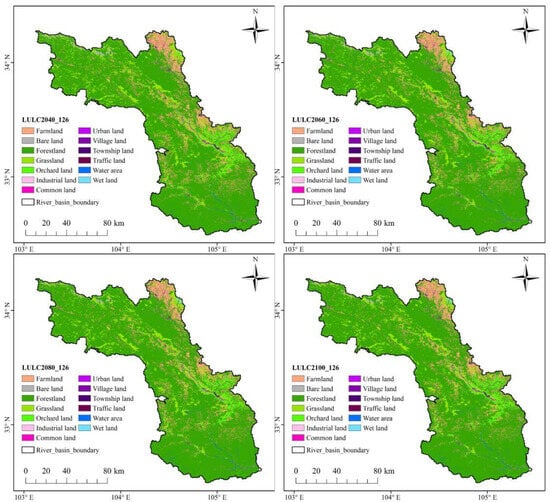
Figure 4.
Land use distribution map under SSP126-EP scenario from 2040–2100 in the BRB.
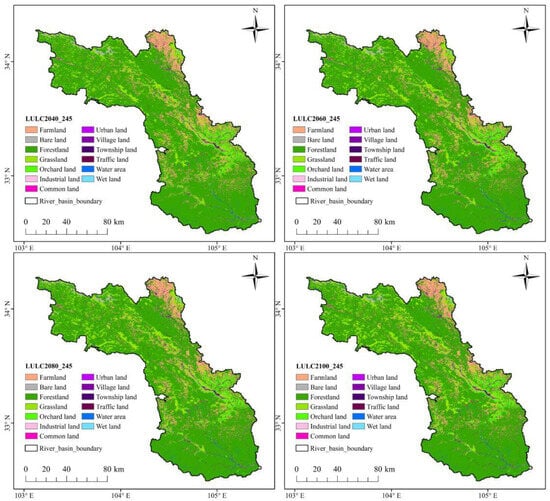
Figure 5.
Land use distribution map under SSP245-ND scenario from 2040–2100 in the BRB.
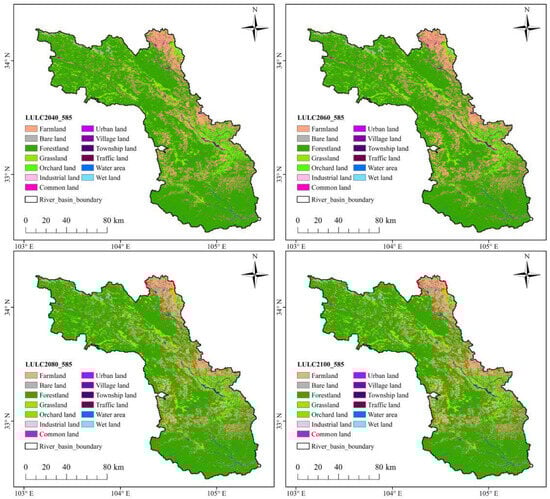
Figure 6.
Land use distribution map under SSP585-EG scenario from 2040–2100 in the BRB.
Under the SSP126-EP scenario, forestland increased by 3.83% from 2040 to 2100, while grassland, farmland, and built-up land decreased by 14.47%, 13.41%, and 23.10%, respectively. Similar to the SSP126-EP scenario, farmland decreases in the SSP245-ND scenario, whereas grassland and built-up land show an increasing trend. Forestland shows a trend of gradual increase and then sudden decrease. Specifically, farmland and forestland decreased by 13.41% and 1.32%, respectively, while grassland and built-up land increased by 14.45% and 24.38%, respectively. In 2040–2100, the forestland area in the SSP585-EG scenario is significantly lower than that in the SSP126-EP and SSP245-ND scenarios. The forestland and grassland decreased by 5.03% and 5.47%, respectively. However, farmland and built-up land increased by 22.42% and 25.81%, respectively.
3.2. Spatiotemporal Distribution of ESs
The distribution of four types of ESs in the BRB shows significant spatial differences. Specifically, the areas with high SC values are mainly located in the Wen County and southeastern regions of the Wudu District. These areas mostly belong to stony mountainous areas or nature reserves with less surface disturbance. The areas with low SC values are distributed on both sides of the Bailong River in the Zhouqu–Wudu–Wen County section where human activities are relatively frequent and industry and agriculture are relatively developed. That is, the low-value SC areas are consistent with areas with high amounts of human activity and areas prone to landslides and debris flows. In the SSP1-2.6 scenario, the basin SC shows an upward trend. Its growth area is mainly concentrated on both sides of the upper reaches of the Bailong River, and the total SC volume increased by 10.38%. In contrast, SC shows a downward trend under the SSP2-4.5 and SSP5-8.5 scenarios, and the declining areas are mainly concentrated between Wudu District and Wen County (Figure 7).
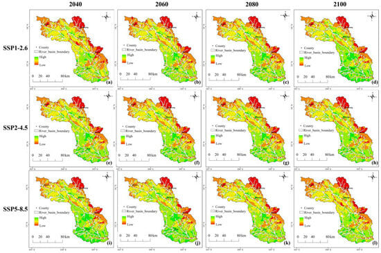
Figure 7.
Spatiotemporal distribution of SC under the SSP1-2.6 scenario (a–d); SSP2-4.5 scenario (e–h); and SSP5-8.5 scenario (i–l) from 2040 to 2100.
Spatially, the distribution pattern of HQ does not change much. Areas with a higher HQ are mainly distributed in nature reserves and forestry management reserves (Figure 8). These include the Baishuijiang National Nature Reserve in Wen County and the Dala, Axia, and Doer Nature Reserves and forestry development zones in Diebu County. The areas with a low HQ are mainly concentrated in river valleys, urban and rural settlements, farming areas, bare land, and low-cover grasslands, where human activities are relatively frequent. The HQ under the SSP1-2.6 scenario is the most elevated, demonstrating a positive trend of escalation, with the most significant increase (3.27%). The HQ of the SSP2-4.5 scenario comes second, also showing increasing change characteristics. The SSP5-8.5 scenario has the worst HQ and shows a significant decreasing trend (−3.19%).
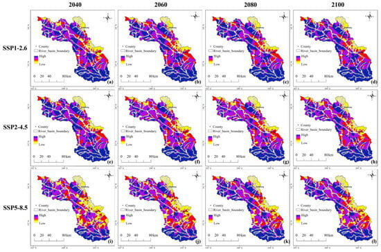
Figure 8.
Spatiotemporal distribution of HQ under the SSP1-2.6 scenario (a–d); SSP2-4.5 scenario (e–h); and SSP5-8.5 scenario (i–l) from 2040 to 2100.
The spatial distribution of the CS across the three scenarios within the BRB exhibits minimal variation, but there are still local changes. Regions exhibiting significantly elevated CS are primarily located in the forested mountainous areas, including the southern mountainous forests of Tanchang County, the high mountainous regions on the southern bank of the Baishui River in Wen County, and the upper to middle reaches of the Boyu River and Gongba River. Low CS value areas are located in agricultural planting areas, towns, high-altitude mountainous areas in Northern Diebu, major landslide areas, and alpine bare-rock areas (Figure 9). This result indicates that forests are the main vegetation type for carbon sequestration, and vegetation coverage has a significant impact on the carbon sequestration function of ecosystems. Within the framework of the SSP1-2.6 scenario, CS within the basin exhibited a significant upward trajectory from 2040 to 2100, with an increase of 3.27 × 10⁶ t, an increase of 12.67%, and the total CS in the entire basin reached 26.06 × 10⁷ t in 2100. The regions experiencing the most significant growth are predominantly located within the Baishui River Basin and the southwestern sector of Wudu District. Under scenarios SSP2-4.5 and SSP5-8.5, CS within the basin exhibited a declining trend over the period from 2040 to 2100, decreasing by 1.64 × 10⁶ t (6.43%) and 5.73 × 10⁶ t (22.86%) respectively. By 2100, the total CS in the entire basin reached 25.33 × 10⁷ t and 24.50 × 10⁷ t, respectively. The areas with reduced CS are primarily concentrated in the northern regions of Wen County and Wudu District.
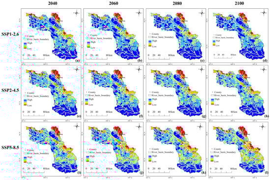
Figure 9.
Spatiotemporal distribution of CS under the SSP1-2.6 scenario (a–d); SSP2-4.5 scenario (e–h); and SSP5-8.5 scenario (i–l) from 2040 to 2100.
The spatial distribution of WY is shown in Figure 10. Under the SSP1-2.6 scenario, the WY is the smallest and shows increasing change characteristics. In the SSP2-4.5 scenario, WY is lower compared to the SSP5-8.5 scenario, with a downward trend observed in both. Under the SSP1-2.6 scenario, the implementation of ecological conservation and restoration projects has successfully mitigated ecological degradation and led to a partial recovery, thereby enhancing the basin’s water production capacity. Within the SSP5-8.5 scenario, extensive regions of grasslands and forests are repurposed as agricultural and urban land, leading to persistent ecosystem degradation, and WY gradually decreases. The spatiotemporal distribution of WY within the basin is intricately linked to precipitation patterns and land use alterations, as evidenced by various studies.
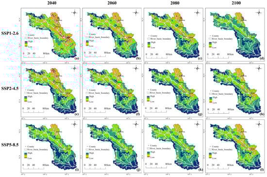
Figure 10.
Spatiotemporal distribution of WY under the SSP1-2.6 scenario (a–d); SSP2-4.5 scenario (e–h); and SSP5-8.5 scenario (i–l) from 2040 to 2100.
3.3. Spatiotemporal Distribution of Trade-Offs/Synergies Between ES Pairs
We performed a Pearson correlation using SPSS20.0 software, and the results are shown in Table 5, Table 6 and Table 7. In the three scenarios, there are synergistic effects among the four ESs. The strongest correlation was observed between CS and HQ, with correlation coefficients exceeding 0.95 (p < 0.01). The SC also showed a significant correlation with HQ, while the correlation between WY and HQ was the weakest, with coefficients below 0.30. However, the changing trends of the correlation coefficients are different over time. Among them, under the SSP1-2.6 scenario, except for the three pairs of ESs related to WY, the correlations of other ESs show a decreasing trend over time. Under the SSP2-4.5 scenario, the correlation between SC-HQ showed a decreasing trend, and the correlation between other ESs exhibited an initial increasing phase followed by a subsequent decline. Under the SSP5-8.5 scenario, the correlation change trend between ESs is more complex. The correlation between CS-HQ shows an increasing trend over time. The correlation between CS-HQ and WY-HQ exhibits a pattern of increasing correlation initially, followed by a subsequent decline, and the correlation between WY-CS shows a decreasing trend. Other ES pairs exhibit an initial negative correlation, which is subsequently followed by a positive correlation over time. Ecosystem service management should prioritize ES pairs characterized by trade-offs, and also consider ES pairs with weakened synergies that imply increased trade-offs [55].
Table 5.
Pearson correlation in the SSP1-2.6 scenario.
Table 6.
Pearson correlation in the SSP2-4.5 scenario.
Table 7.
Pearson correlation in the SSP5-8.5 scenario.
The spatial correlations among ESs are illustrated in Figure 11. The spatial correlation of the three scenarios shows significant differences. Among them, under the SSP1-2.6 scenario, most ESs show synergistic effects, and the proportion of catchments showing synergistic effects reaches more than 82%. SC-WY had the largest proportion of synergistic effects (99.45%), followed by HQ-CS (90.48%). The region exhibiting the highest intensity of synergistic effects is predominantly situated in the central part of the basin. Under the SSP2-4.5 scenario, the proportion of channels showing synergistic effects between SC and WY is 97.98%. The proportion of areas exhibiting synergistic effects between HQ and CS constitutes 32.24%, mainly distributed in Wudu District. The proportions of channels showing good effects for HQ-SC and HQ-WY were 43.58% and 43.48% respectively, concentrated in Wen County and Wudu District in the southern part of the basin. Under the SSP5-8.5 scenario, the channels showing synergistic effects between HQ and CS account for the largest proportion (85.39%). The proportions of channels showing synergistic effects of HQ-SC and SC-CS accounted for 70.43% and 75.47%, respectively, with these areas predominantly found across the central and southern regions of the basin. The proportion of channels showing a trade-off effect for HQ-WY is as high as 87.66%, which is distributed throughout the basin. The proportion of channels showing trade-off effects for SC-WY and CS-WY is as high as 85.14% and 71.32%, respectively, and the correlation gradually increases from southwest to northeast. Consequently, it is imperative for managers to be cognizant of these dynamics and to implement suitable interventions [49]. Promote ES improvement by avoiding unnecessary ES correlations.
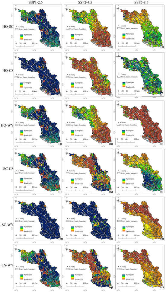
Figure 11.
Spatial correlation distribution of (a–c) HQ and SC; (d–f) HQ and CS; (g–i) HQ and WY; (j–l) SC and CS; (m–o) SC and WY; (p–r) CS and WY in the BRB under SSP1-2.6, SSP2-4.5, and SSP5-8.5 scenarios.
3.4. Spatial Distribution Characteristics of ES Bundles
The SOM identified six ES bundles at the sub-basin scale (Figure 12). The ES bundle refers to a collection of different ES aggregation distributions in space or time [54]. The spatial distribution patterns of ES bundles exhibit substantial variability across distinct scenarios. For Cluster 1, this cluster is situated along the banks of the Bailong River within the urban boundaries of the Wudu District. Under the SSP1-2.6 scenario, SSP2-4.5 scenario, and SSP5-8.5 scenario, they account for 20.34%, 12.29%, and 13.39% of the basin, respectively. This ES bundle is distinguished by the spatial synergy between HQ and CS, featuring elevated levels of both services. For Cluster 2, this bundle mainly covers the northern area of Tanchang County, covering 6.04%, 7.55%, and 10.78% of the basin area in the SSP1-2.6 scenario, SSP2-4.5 scenario and SPP5-8.5 scenario, respectively. This bundle provides weak Ess, except for WY. For Cluster 3, this cluster is predominantly situated along the left bank of the Bailong River within Zhouqu County and spans the northern region of Diebu County. Under the SSP1-2.6 scenario, SSP2-4.5 scenario, and SPP5-8.5 scenario, they account for 9.11%, 12.84%, and 14.10% of the basin area, respectively. This ES bundle demonstrates spatial synergies, characterized by high levels of CS, HQ, and WY. For Cluster 4, this cluster is predominantly situated in the regions with more favorable ecological conditions located in the southern part of the basin, with the largest proportion under the SSP1-2.6 scenario (20.29%), followed by the SSP2-4.5 scenario (18.33%). The SSP5-8.5 scenario accounts for the smallest proportion (18.13%). This bundle mainly focuses on the balanced development of four ESs, especially in the SSP1-2.6 scenario. For Cluster 5, this cluster is primarily distributed along the banks of the Bailong River, spanning both Diebu County and Zhouqu County. The three scenarios account for 25.08%, 26.44%, and 23.31% of the basin, respectively. This bundle is distinguished by the spatial synergy among high CS, high HQ, and elevated SC. For Cluster 6, this cluster comprises sub-basins situated in the eastern and southern hilly regions. Under the three scenarios, this cluster accounts for 19.13%, 22.56%, and 19.76% of the watershed, respectively. This bundle is characterized by the balanced development of the other three ESs except SC (Figure 13).
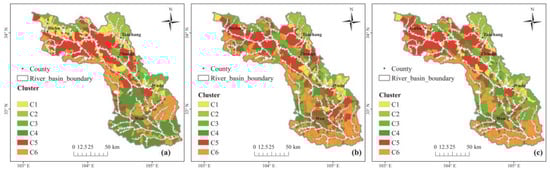
Figure 12.
The spatial distribution pattern of ES bundles at the sub-basin scale under (a) SSP1-2.6; (b) SSP2-4.5; and (c) SSP5-8.5 scenarios. Note: The pie chart represents the number of sub-basins in each ES bundle, with more red indicating a higher number of sub-basins.
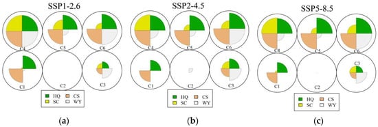
Figure 13.
Composition and relative magnitude of ESs in ES bundles at the sub-basin scale under (a) SSP1-2.6; (b) SSP2-4.5; and (c) SSP5-8.5 scenarios. Note: longer segments represent higher ES supply.
4. Discussion
4.1. Analysis of the Impact of Land Use on ES
The spatial distribution of land use in the BRB exhibits significant differences under different climate models and development strategies. The changes in the area of built-up land and farmland differ across the three scenarios. In the SSP126-EP scenario, built-up land decreases, while forest area increases to achieve ecological sustainability [56]. In the SSP585-EG scenario, the amount of land available for construction increases significantly due to socioeconomic factors. This trend is similar to the historical patterns observed in the SSP245-ND scenario [57]. By comparison, it is shown that the expansion of built-up land is more influenced by economic development, while the increase in farmland area is mainly affected by population growth [58,59]. In addition, by comparing the changes in forestland area, lower economic growth rates and more stable climate environments are conducive to the expansion of the forestland area, and forests often extend to areas with better ecological environments [60], which is similar to our results. Therefore, to ensure the stability of regional ecosystems and achieve sustainable development, policies must be formulated to strictly regulate the unchecked expansion of built-up land, strengthening the protection of ecological lands (water bodies, forestland, and grassland) [61].
Previous studies have indicated that vegetation has significant impacts on ESs, such as SC, WY, CS, and HQ [62,63]. Wang et al. found that the trade-off/synergy between NPP, SR, and WY varies under different climate and land use conditions in Shaanxi Province [64]. Research has shown that ecological restoration projects have an improving effect on WY, SR, and CS in the Loess Plateau of Northern Shaanxi and can also affect changes in ES bundles. Moreover, the significant synergistic enhancement in SR and CS suggests ecological amelioration [65]. The BRB is situated in a transitional ecological zone and frequently experiences geological disasters, such as landslides, mudslides, and floods. Land use is inefficient, and land degradation is severe. Our predictions align with the trends observed in other related studies. The SSP1-2.6 scenario is a relatively idealized scenario that provides the most dense and efficient ESs, suppresses rapid urban expansion, increases ecological land use, and enhances all four ESs to varying degrees. However, in the SSP2-4.5 and SSP5-8.5 scenarios, it is expected that climate change and land use changes will be more severe, resulting in greater ES losses under higher development pressures [34]. These results indicate that implementing ecological protection measures can reduce land use changes caused by human activities and increase ecosystem functions [66]. Variations in population size and agricultural development are the principal drivers of LUCC. Within the SSP5-8.5 scenario, population expansion and economic progress have resulted in a notable escalation of urban and built-up land areas, which are concurrent with a reduction in forestland, and these LUCCs have exerted adverse effects on ESs [67]. This conclusion is consistent with the research results of Zhang et al. [68].
4.2. Suggestions on the Management of ES in the BRB
The ultimate goal of ESs is their practical application, providing a theoretical basis and technical support for the management of regional ESs and environmental protection [69]. The maintenance of ESs is vital to the future of humanity. However, ecosystem degradation is common and often triggers further disasters, reducing the resilience of natural and socioeconomic systems to climate change and irrational human activities. The current research on protecting the natural capital of ecosystems is still in its infancy [70]. The pressing challenge is to translate ideas into action through social policy and decision-making [71]. The goal of the current research is to implement ecological environment management within different ES functional areas and enhance human activities that are crucial to the ecological environment through land use policy formulation and governance.
Mountainous regions are deemed optimal for studying the effects of LUCC on ESs. On one hand, their unique topography enables mountain regions to effectively store and filter diverse material and energy flows [72]. With unique geological, geomorphological, climatic, hydrological, and other environmental features, mountains nurture diverse ecosystems and provide a variety of ESs to local residents [73]. On the other hand, mountain areas are vulnerable regions and frequently experience disasters, such as landslides and mudflows. The population in mountainous areas of China is relatively large, and these regions are undergoing rapid industrialization and urbanization. So, the relationship between LUCC and ES seems more complex in mountainous areas. Meanwhile, a series of policies are being implemented in these areas, such as “Reform and Opening-up” and “Western Development”, aimed at promoting local economic growth, as well as “Grain for Green” policies designed to strengthen ecological protection. The above policies have all promoted regional land use change. In future development, mountain areas should focus on coordinating ecological protection with economic development. Regional economic development has shifted from “high-speed” development to “high-quality” development to enhance the value of ES in the research area.
The BRB is a fragile mountainous area prone to natural disasters. We combine the ES spatiotemporal trade-off/synergy status and ecological zoning to put forward relevant suggestions and measures with the goal of protecting people’s lives and property, reducing disaster hazards, and promoting regional sustainable development. Therefore, in regional land use planning, priority must be given to WY. The WY in some areas on both sides of the Bailong River is showing an increasing trend, which will increase the risk of landslides and debris flow disasters (C3). In these areas, relevant departments should strengthen the construction of disaster prevention and early-warning projects [74]. In the southern region where forestland was restored, there were relatively more areas with increased ESs (C4). Therefore, the implementation of extensive plantations in the south should be considered to improve the capacity of ESs such as SC and CS. In addition, in ecologically fragile gully areas (C5), afforestation projects should weigh the pros and cons, and the expansion of construction land should be controlled within an appropriate range. We suggest focusing on the extreme aggregation of high ESs in future development.
4.3. Shortcomings and Prospects
Our study encounters certain limitations. First, the complexity of LUCC brings a certain degree of uncertainty to land use simulation. The changes in land use are not only influenced by spatially expressive factors such as economy and population but also by policy frameworks including farmland protection and ecological protection regulations [75,76,77]. Secondly, climate and land use changes have different impacts on different ecosystems. In this study, we investigated four typical ES: SC, WY, CS, and HQ. We did not assess other services, including cultural services, due to constraints on data availability and simulation methodologies. Considering LUCC and climate change, the inclusion of a broader range of ESs could facilitate a more holistic investigation into the mechanisms of ES changes in future studies. We should choose more indicators to simulate important ESs. Finally, we simulated multiple ESs under the combined effects of LUCC and climate change, which helps to better understand ES dynamics. We incorporate climate change into the LUCC simulations, which makes the assessment of future ESs more realistic. It is imperative to delineate the independent impacts of these two primary drivers in future studies to ascertain their relative strength and dominance across various ESs [78]. Such discernment is vital for the effective integration of planning and policy-making [79].
5. Conclusions
This study coupled the PLUS and InVEST models to simulate LUCC and ESs and their mutual relationships under different SSP-RCP scenarios. Under the SSP126-EP scenario, the forestland expanded rapidly, and the grassland, farmland, and built-up land will decrease. In the SSP245-ND scenario, the land use change pattern is similar to that in the SSP126-EP scenario, but the growth of forest land is slow. Under the SSP585-EG scenario, built-up land and farmland expanded rapidly. From 2040 to 2100, all four ESs increase under the SSP1-2.6 scenario. Under the SSP2-4.5 and SSP5-8.5 scenarios, ESs show a decreasing trend. There are synergistic effects between ES pairs, and attention should be paid to ES pairs with reduced synergistic effects. The cluster with a balanced development of the four ESs is situated in the southern region of the basin, and this cluster accounts for the highest proportion in the SSP1-2.6 scenario. Clusters with weak ESs are mainly situated in the northern area of Tanchang County, and this cluster has the highest proportion in the SSP5-8.5 scenario. We recommend the development of spatial planning and management strategies that are informed by the trade-offs/synergies among ES, as well as the specific bundles of ESs, to promote the sustainable development of regional ecosystems.
Author Contributions
Conceptualization, S.L. and Y.Z.; methodology, S.L. and Z.L.; software, S.L. and Z.L.; validation, Y.Z., D.Y. and Z.G.; formal analysis, S.L.; investigation, S.L.; resources, S.L. and Y.Z.; data curation, S.L. and Y.Z.; writing—original draft preparation, S.L.; writing—review and editing, S.L. and Y.Z.; visualization, S.L.; supervision, D.Y.; project administration, D.Y.; funding acquisition, D.Y. All authors have read and agreed to the published version of the manuscript.
Funding
This work was supported by the Science Foundation of Hebei Normal University (Grant No. L2024B26), Major Scientific and Technological Projects of Gansu Province (Grant No. 22ZD6FA051), the National Natural Science Foundation of China (Grant Nos. 42077230), and the Second Tibetan Plateau Scientific Expedition and Research program (Grant No. 2021QZKK0204).
Data Availability Statement
The raw data supporting the conclusions of this article will be made available by the authors on request.
Conflicts of Interest
The authors declare no conflicts of interest.
References
- Fu, B.; Wang, S.; Su, C.; Forsius, M. Linking Ecosystem Processes and Ecosystem Services. Curr. Opin. Environ. Sustain. 2013, 5, 4–10. [Google Scholar] [CrossRef]
- Costanza, R.; De Groot, R.; Braat, L.; Kubiszewski, I.; Fioramonti, L.; Sutton, P.; Farber, S.; Grasso, M. Twenty Years of Ecosystem Services: How Far Have We Come and How Far Do We Still Need to Go? Ecosyst. Serv. 2017, 28, 1–16. [Google Scholar] [CrossRef]
- Gong, Z.; Liu, W.; Guo, J.; Su, Y.; Gao, Y.; Bu, W.; Ren, J.; Li, C. How to Achieve the Ecological Sustainability Goal of Ecologically Fragile Areas on the Qinghai-Tibet Plateau: A Multi-Scenario Simulation of Lanzhou-Xining Urban Agglomerations. Land 2024, 13, 1730. [Google Scholar] [CrossRef]
- Escobedo, F.J.; Kroeger, T.; Wagner, J.E. Urban Forests and Pollution Mitigation: Analyzing Ecosystem Services and Disservices. Env. Pollut. 2011, 159, 2078–2087. [Google Scholar] [CrossRef] [PubMed]
- Bussmann, R. Destruction and Management of Mount Kenya’s Forests. AMBIO A J. Hum. Environ. 1996, 25, 314–317. [Google Scholar]
- de Araujo Barbosa, C.C.; Atkinson, P.M.; Dearing, J.A. Extravagance in the Commons: Resource Exploitation and the Frontiers of Ecosystem Service Depletion in the Amazon Estuary. Sci. Total Environ. 2016, 550, 6–16. [Google Scholar] [CrossRef]
- Dadashpoor, H.; Azizi, P.; Moghadasi, M. Land Use Change, Urbanization, and Change in Landscape Pattern in a Metropolitan Area. Sci. Total Environ. 2019, 655, 707–719. [Google Scholar] [CrossRef]
- Grimm, N.B.; Groffman, P.; Staudinger, M.; Tallis, H. Climate Change Impacts on Ecosystems and Ecosystem Services in the United States: Process and Prospects for Sustained Assessment. Clim. Chang. 2016, 135, 97–109. [Google Scholar] [CrossRef]
- Fulford, R.S.; Russell, M.; Myers, M.; Malish, M.; Delmaine, A. Models Help Set Ecosystem Service Baselines for Restoration Assessment. J. Environ. Manag. 2022, 317, 115411. [Google Scholar] [CrossRef]
- Mu, L.; Fang, L.; Dou, W.; Wang, C.; Qu, X.; Yu, Y. Urbanization-Induced Spatio-Temporal Variation of Water Resources Utilization in Northwestern China: A Spatial Panel Model Based Approach. Ecol. Indic. 2021, 125, 107457. [Google Scholar] [CrossRef]
- Liu, X.; Sun, T.; Feng, Q. Dynamic Spatial Spillover Effect of Urbanization on Environmental Pollution in China Considering the Inertia Characteristics of Environmental Pollution. Sustain. Cities Soc. 2020, 53, 101903. [Google Scholar] [CrossRef]
- Behboudian, M.; Kerachian, R.; Motlaghzadeh, K.; Ashrafi, S. Application of Multi-Agent Decision-Making Methods in Hydrological Ecosystem Services Management. MethodsX 2023, 10, 102130. [Google Scholar] [CrossRef] [PubMed]
- Bagyaraj, M.; Senapathi, V.; Karthikeyan, S.; Chung, S.Y.; Khatibi, R.; Nadiri, A.A.; Asgari Lajayer, B. A Study of Urban Heat Island Effects Using Remote Sensing and GIS Techniques in Kancheepuram, Tamil Nadu, India. Urban Clim. 2023, 51, 101597. [Google Scholar] [CrossRef]
- Dibs, H.; Sabah Jaber, H.; Al-Ansari, N. Multi-Fusion Algorithms for Detecting Land Surface Pattern Changes Using Multi-High Spatial Resolution Images and Remote Sensing Analysis. Emerg. Sci. J. 2023, 7, 1215–1231. [Google Scholar] [CrossRef]
- Ding, Q.; Wang, L.; Fu, M.; Huang, N. An Integrated System for Rapid Assessment of Ecological Quality Based on Remote Sensing Data. Environ. Sci. Pollut. Res. 2020, 27, 32779–32795. [Google Scholar] [CrossRef]
- Dibs, H.; Abed, S.A.; Ali, A.H.; Al-Ansari, N. Fusion Landsat-8 Thermal TIRS and OLI Datasets for Superior Monitoring and Change Detection Using Remote Sensing. Emerg. Sci. J. 2023, 7, 428–444. [Google Scholar] [CrossRef]
- Pereira, P. Ecosystem Services in a Changing Environment. Sci. Total Environ. 2020, 702, 135008. [Google Scholar] [CrossRef]
- Ran, P.; Hu, S.; Frazier, A.E.; Yang, S.; Song, X.; Qu, S. The Dynamic Relationships between Landscape Structure and Ecosystem Services: An Empirical Analysis from the Wuhan Metropolitan Area, China. J. Environ. Manag. 2023, 325, 116575. [Google Scholar] [CrossRef]
- Arunyawat, S.; Shrestha, R.P. Assessing Land Use Change and Its Impact on Ecosystem Services in Northern Thailand. Sustainability 2016, 8, 768. [Google Scholar] [CrossRef]
- Yang, Y. Evolution of Habitat Quality and Association with Land-Use Changes in Mountainous Areas: A Case Study of the Taihang Mountains in Hebei Province, China. Ecol. Indic. 2021, 129, 107967. [Google Scholar] [CrossRef]
- Li, M.; Liang, D.; Xia, J.; Song, J.; Cheng, D.; Wu, J.; Cao, Y.; Sun, H.; Li, Q. Evaluation of Water Conservation Function of Danjiang River Basin in Qinling Mountains, China Based on InVEST Model. J. Environ. Manag. 2021, 286, 112212. [Google Scholar] [CrossRef] [PubMed]
- Yang, Y.; Li, H.; Qian, C. Analysis of the Implementation Effects of Ecological Restoration Projects Based on Carbon Storage and Eco-Environmental Quality: A Case Study of the Yellow River Delta, China. J. Environ. Manag. 2023, 340, 117929. [Google Scholar] [CrossRef]
- Huang, H.; Xue, J.; Feng, X.; Zhao, J.; Sun, H.; Hu, Y.; Ma, Y. Thriving arid oasis urban agglomerations: Optimizing ecosystem services pattern under future climate change scenarios using dynamic Bayesian network. J. Environ. Manag. 2024, 350, 119612. [Google Scholar] [CrossRef] [PubMed]
- Yuan, M.-H.; Lo, S.-L. Ecosystem Services and Sustainable Development: Perspectives from the Food-Energy-Water Nexus. Ecosyst. Serv. 2020, 46, 101217. [Google Scholar] [CrossRef]
- Long, H.; Qu, Y. Land Use Transitions and Land Management: A Mutual Feedback Perspective. Land Use Policy 2018, 74, 111–120. [Google Scholar] [CrossRef]
- Wang, M.; Sun, X. Potential Impact of Land Use Change on Ecosystem Services in China. Environ. Monit. Assess. 2016, 188, 248. [Google Scholar] [CrossRef]
- Quintas-Soriano, C.; Castro, A.J.; Castro, H.; García-Llorente, M. Impacts of Land Use Change on Ecosystem Services and Implications for Human Well-Being in Spanish Drylands. Land Use Policy 2016, 54, 534–548. [Google Scholar] [CrossRef]
- Bera, D.; Chatterjee, N.D.; Dinda, S.; Ghosh, S.; Dhiman, V.; Bashir, B.; Calka, B.; Zhran, M. Assessment of Carbon Stock and Sequestration Dynamics in Response to Land Use and Land Cover Changes in a Tropical Landscape. Land 2024, 13, 1689. [Google Scholar] [CrossRef]
- Doelman, J.C.; Stehfest, E.; Tabeau, A.; van Meijl, H.; Lassaletta, L.; Gernaat, D.E.H.J.; Hermans, K.; Harmsen, M.; Daioglou, V.; Biemans, H.; et al. Exploring SSP Land-Use Dynamics Using the IMAGE Model: Regional and Gridded Scenarios of Land-Use Change and Land-Based Climate Change Mitigation. Glob. Environ. Chang. 2018, 48, 119–135. [Google Scholar] [CrossRef]
- Kebede, A.S.; Nicholls, R.J.; Allan, A.; Arto, I.; Cazcarro, I.; Fernandes, J.A.; Hill, C.T.; Hutton, C.W.; Kay, S.; Lázár, A.N.; et al. Applying the Global RCP–SSP–SPA Scenario Framework at Sub-National Scale: A Multi-Scale and Participatory Scenario Approach. Sci. Total Environ. 2018, 635, 659–672. [Google Scholar] [CrossRef]
- Eyring, V.; Bony, S.; Meehl, G.A.; Senior, C.A.; Stevens, B.; Stouffer, R.J.; Taylor, K.E. Overview of the Coupled Model Intercomparison Project Phase 6 (CMIP6) Experimental Design and Organization. Geosci. Model Dev. 2016, 9, 1937–1958. [Google Scholar] [CrossRef]
- Dong, N.; You, L.; Cai, W.; Li, G.; Lin, H. Land Use Projections in China under Global Socioeconomic and Emission Scenarios: Utilizing a Scenario-Based Land-Use Change Assessment Framework. Glob. Environ. Chang. 2018, 50, 164–177. [Google Scholar] [CrossRef]
- Qiu, Y.; Feng, J.; Yan, Z.; Wang, J. Assessing the Land-Use Harmonization (LUH) 2 Dataset in Central Asia for Regional Climate Model Projection. Environ. Res. Lett. 2023, 18, 064008. [Google Scholar] [CrossRef]
- Guo, W.; Teng, Y.; Li, J.; Yan, Y.; Zhao, C.; Li, Y.; Li, X. A New Assessment Framework to Forecast Land Use and Carbon Storage under Different SSP-RCP Scenarios in China. Sci. Total Environ. 2024, 912, 169088. [Google Scholar] [CrossRef]
- Li, J.; Chen, X.; Kurban, A.; Van de Voorde, T.; De Maeyer, P.; Zhang, C. Coupled SSPs-RCPs scenarios to project the future dynamic variations of water-soil-carbon-biodiversity services in Central Asia. Ecol. Indic. 2021, 129, 107936. [Google Scholar] [CrossRef]
- Shi, X.; Matsui, T.; Machimura, T.; Haga, C.; Hu, A.; Gan, X. Impact of Urbanization on the Food–Water–Land–Ecosystem Nexus: A Study of Shenzhen, China. Sci. Total Environ. 2022, 808, 152138. [Google Scholar] [CrossRef]
- Wu, J.; Luo, J.; Zhang, H.; Qin, S.; Yu, M. Projections of Land Use Change and Habitat Quality Assessment by Coupling Climate Change and Development Patterns. Sci. Total Environ. 2022, 847, 157491. [Google Scholar] [CrossRef]
- Gong, J.; Liu, D.; Zhang, J.; Xie, Y.; Cao, E.; Li, H. Tradeoffs/Synergies of Multiple Ecosystem Services Based on Land Use Simulation in a Mountain-Basin Area, Western China. Ecol. Indic. 2019, 99, 283–293. [Google Scholar] [CrossRef]
- Luo, Y.; Yang, D.; O’Connor, P.; Wu, T.; Ma, W.; Xu, L.; Guo, R.; Lin, J. Dynamic Characteristics and Synergistic Effects of Ecosystem Services under Climate Change Scenarios on the Qinghai–Tibet Plateau. Sci. Rep. 2022, 12, 2540. [Google Scholar] [CrossRef]
- Yin, Z.; Fu, X.; Sun, R.; Li, S.; Tang, M.; Deng, H.; Wu, G. Spatially Heterogeneous Relationships between Ecosystem Service Trade-Offs and Their Driving Factors: A Case Study in Baiyangdian Basin, China. Land 2024, 13, 1619. [Google Scholar] [CrossRef]
- Zheng, H.; Li, Y.; Ouyang, Z.; Luo, Y. Progress and Perspectives of Ecosystem Services Management. Acta Ecol. Sin. 2013, 33, 702–710. [Google Scholar] [CrossRef]
- Han, P.; Yang, G.; Wang, Z.; Liu, Y.; Chen, X.; Zhang, W.; Zhang, Z.; Wen, Z.; Shi, H.; Lin, Z.; et al. Driving Factors and Trade-Offs/Synergies Analysis of the Spatiotemporal Changes of Multiple Ecosystem Services in the Han River Basin, China. Remote Sens. 2024, 16, 2115. [Google Scholar] [CrossRef]
- Geneletti, D. Assessing the Impact of Alternative Land-Use Zoning Policies on Future Ecosystem Services. Environ. Impact Assess. Rev. 2013, 40, 25–35. [Google Scholar] [CrossRef]
- Divinsky, I.; Becker, N.; Bar (Kutiel), P. Ecosystem Service Tradeoff between Grazing Intensity and Other Services—A Case Study in Karei-Deshe Experimental Cattle Range in Northern Israel. Ecosyst. Serv. 2017, 24, 16–27. [Google Scholar] [CrossRef]
- Jiang, W.; Chen, G.; Meng, X.; Jin, J.; Zhao, Y.; Lin, L.; Li, Y.; Zhang, Y. Probabilistic Rainfall Threshold of Landslides in Data-Scarce Mountainous Areas: A Case Study of the Bailong River Basin, China. Catena 2022, 213, 106190. [Google Scholar] [CrossRef]
- Liang, X.; Guan, Q.; Clarke, K.C.; Liu, S.; Wang, B.; Yao, Y. Understanding the Drivers of Sustainable Land Expansion Using a Patch-Generating Land Use Simulation (PLUS) Model: A Case Study in Wuhan, China. Comput. Environ. Urban Syst. 2021, 85, 101569. [Google Scholar] [CrossRef]
- Shan, X.; Yin, J.; Wang, J. Risk Assessment of Shanghai Extreme Flooding under the Land Use Change Scenario. Nat. Hazards 2022, 110, 1039–1060. [Google Scholar] [CrossRef]
- Lin, Q.; Wang, Y.; Glade, T.; Zhang, J.; Zhang, Y. Assessing the Spatiotemporal Impact of Climate Change on Event Rainfall Characteristics Influencing Landslide Occurrences Based on Multiple GCM Projections in China. Clim. Chang. 2020, 162, 761–779. [Google Scholar] [CrossRef]
- Zhang, Y.; Wu, T.; Song, C.; Hein, L.; Shi, F.; Han, M.; Ouyang, Z. Influences of Climate Change and Land Use Change on the Interactions of Ecosystem Services in China’s Xijiang River Basin. Ecosyst. Serv. 2022, 58, 101489. [Google Scholar] [CrossRef]
- Yue, D.; Zhou, Y.; Guo, J.; Chao, Z.; Liang, G.; Zheng, X. Ecosystem Service Evaluation and Optimisation in the Shule River Basin, China. Catena 2022, 215, 106320. [Google Scholar] [CrossRef]
- Gong, J.; Jin, T.; Liu, D.; Zhu, Y.; Yan, L. Are Ecosystem Service Bundles Useful for Mountainous Landscape Function Zoning and Management? A Case Study of Bailongjiang Watershed in Western China. Ecol. Indic. 2022, 134, 108495. [Google Scholar] [CrossRef]
- Xu, L.; He, N.; Yu, G. A Dataset of Carbon Density in Chinese Terrestrial Ecosystems (2010s). CSD 2018, 4. [Google Scholar] [CrossRef]
- Chen, L.; Yao, Y.; Xiang, K.; Dai, X.; Li, W.; Dai, H.; Lu, K.; Li, W.; Lu, H.; Zhang, Y.; et al. Spatial-Temporal Pattern of Ecosystem Services and Sustainable Development in Representative Mountainous Cities: A Case Study of Chengdu-Chongqing Urban Agglomeration. J. Environ. Manag. 2024, 368, 122261. [Google Scholar] [CrossRef] [PubMed]
- Raudsepp-Hearne, C.; Peterson, G.D.; Bennett, E.M. Ecosystem Service Bundles for Analyzing Tradeoffs in Diverse Landscapes. Proc. Natl. Acad. Sci. USA 2010, 107, 5242–5247. [Google Scholar] [CrossRef]
- Xia, H.; Yuan, S.; Prishchepov, A.V. Spatial-Temporal Heterogeneity of Ecosystem Service Interactions and Their Social-Ecological Drivers: Implications for Spatial Planning and Management. Resour. Conserv. Recycl. 2023, 189, 106767. [Google Scholar] [CrossRef]
- Xu, C.; Jiang, Y.; Su, Z.; Liu, Y.; Lyu, J. Assessing the Impacts of Grain-for-Green Programme on Ecosystem Services in Jinghe River Basin, China. Ecol. Indic. 2022, 137, 108757. [Google Scholar] [CrossRef]
- Gomes, E.; Inácio, M.; Bogdzevič, K.; Kalinauskas, M.; Karnauskaitė, D.; Pereira, P. Future Land-Use Changes and Its Impacts on Terrestrial Ecosystem Services: A Review. Sci. Total Environ. 2021, 781, 146716. [Google Scholar] [CrossRef]
- Tan, M.; Li, X.; Xie, H.; Lu, C. Urban Land Expansion and Arable Land Loss in China—A Case Study of Beijing–Tianjin–Hebei Region. Land Use Policy 2005, 22, 187–196. [Google Scholar] [CrossRef]
- Zhang, Y.; Xie, H. Interactive Relationship among Urban Expansion, Economic Development, and Population Growth since the Reform and Opening up in China: An Analysis Based on a Vector Error Correction Model. Land 2019, 8, 153. [Google Scholar] [CrossRef]
- Weisberg, P.J.; Lingua, E.; Pillai, R.B. Spatial Patterns of Pinyon–Juniper Woodland Expansion in Central Nevada. Rangel. Ecol. Manag. 2007, 60, 115–124. [Google Scholar] [CrossRef]
- Cen, X.; Zhang, H. Impacts of Multi-Scenario Land Use Change on Ecosystem Services and Ecological Security Pattern: A Case Study of the Yellow River Delta. Res. Cold Arid Reg. 2024, 16, 30–44. [Google Scholar] [CrossRef]
- Lyu, R.; Clarke, K.C.; Zhang, J.; Feng, J.; Jia, X.; Li, J. Spatial Correlations among Ecosystem Services and Their Socio-Ecological Driving Factors: A Case Study in the City Belt along the Yellow River in Ningxia, China. Appl. Geogr. 2019, 108, 64–73. [Google Scholar] [CrossRef]
- Wen, X.; Deng, X.; Zhang, F. Scale Effects of Vegetation Restoration on Soil and Water Conservation in a Semi-Arid Region in China: Resources Conservation and Sustainable Management. Resour. Conserv. Recycl. 2019, 151, 104474. [Google Scholar] [CrossRef]
- Wang, H.; Liu, G.; Li, Z.; Zhang, L.; Wang, Z. Processes and Driving Forces for Changing Vegetation Ecosystem Services: Insights from the Shaanxi Province of China. Ecol. Indic. 2020, 112, 106105. [Google Scholar] [CrossRef]
- Lyu, F.; Tang, J.; Olhnuud, A.; Hao, F.; Gong, C. The Impact of Large-Scale Ecological Restoration Projects on Trade-Offs/Synergies and Clusters of Ecosystem Services. J. Environ. Manag. 2024, 365, 121591. [Google Scholar] [CrossRef]
- Zhu, L.; Song, R.; Sun, S.; Li, Y.; Hu, K. Land Use/Land Cover Change and Its Impact on Ecosystem Carbon Storage in Coastal Areas of China from 1980 to 2050. Ecol. Indic. 2022, 142, 109178. [Google Scholar] [CrossRef]
- Hasan, S.S.; Zhen, L.; Miah, M.G.; Ahamed, T.; Samie, A. Impact of Land Use Change on Ecosystem Services: A Review. Environ. Dev. 2020, 34, 100527. [Google Scholar] [CrossRef]
- Zhang, X.Y.; Zhang, X.; Li, D.H.; Lu, L.; Yu, H. Multi-scenario simulation of the impact of urban land use change on ecosystem service value in Shenzhen. Acta Ecol. Sin. 2022, 42, 2086–2097. [Google Scholar]
- Gong, J.; Cao, E.; Xie, Y.; Xu, C.; Li, H.; Yan, L. Integrating Ecosystem Services and Landscape Ecological Risk into Adaptive Management: Insights from a Western Mountain-Basin Area, China. J. Environ. Manag. 2021, 281, 111817. [Google Scholar] [CrossRef]
- Goldstein, J.H.; Caldarone, G.; Duarte, T.K.; Ennaanay, D.; Hannahs, N.; Mendoza, G.; Polasky, S.; Wolny, S.; Daily, G.C. Integrating Ecosystem-Service Tradeoffs into Land-Use Decisions. Proc. Natl. Acad. Sci. USA 2012, 109, 7565–7570. [Google Scholar] [CrossRef]
- Daily, G.C.; Polasky, S.; Goldstein, J.; Kareiva, P.M.; Mooney, H.A.; Pejchar, L.; Ricketts, T.H.; Salzman, J.; Shallenberger, R. Ecosystem Services in Decision Making: Time to Deliver. Front. Ecol. Environ. 2009, 7, 21–28. [Google Scholar] [CrossRef]
- Zhang, M.; Wang, K.; Liu, H.; Zhang, C.; Yue, Y.; Qi, X. Effect of Ecological Engineering Projects on Ecosystem Services in a Karst Region: A Case Study of Northwest Guangxi, China. J. Clean. Prod. 2018, 183, 831–842. [Google Scholar] [CrossRef]
- Egarter Vigl, L.; Schirpke, U.; Tasser, E.; Tappeiner, U. Linking Long-Term Landscape Dynamics to the Multiple Interactions among Ecosystem Services in the European Alps. Landsc. Ecol. 2016, 31, 1903–1918. [Google Scholar] [CrossRef]
- Wang, S.; Zhang, L.; She, D.; Wang, G.; Zhang, Q. Future Projections of Flooding Characteristics in the Lancang-Mekong River Basin under Climate Change. J. Hydrol. 2021, 602, 126778. [Google Scholar] [CrossRef]
- Liang, X.; Liu, X.; Li, D.; Zhao, H.; Chen, G. Urban Growth Simulation by Incorporating Planning Policies into a CA-Based Future Land-Use Simulation Model. Int. J. Geogr. Inf. Sci. 2018, 32, 2294–2316. [Google Scholar] [CrossRef]
- Tan, R.; Liu, P.; Zhou, K.; He, Q. Evaluating the Effectiveness of Development-Limiting Boundary Control Policy: Spatial Difference-in-Difference Analysis. Land Use Policy 2022, 120, 106229. [Google Scholar] [CrossRef]
- Yang, H.; Huang, X.; Thompson, J.R.; Flower, R.J. Enforcement Key to China’s Environment. Science 2015, 347, 834–835. [Google Scholar] [CrossRef]
- Li, L.; Huang, X.; Wu, D.; Yang, H. Construction of Ecological Security Pattern Adapting to Future Land Use Change in Pearl River Delta, China. Appl. Geogr. 2023, 154, 102946. [Google Scholar] [CrossRef]
- Sun, L.; Yu, H.; Sun, M.; Wang, Y. Coupled Impacts of Climate and Land Use Changes on Regional Ecosystem Services. J. Environ. Manag. 2023, 326, 116753. [Google Scholar] [CrossRef]
Disclaimer/Publisher’s Note: The statements, opinions and data contained in all publications are solely those of the individual author(s) and contributor(s) and not of MDPI and/or the editor(s). MDPI and/or the editor(s) disclaim responsibility for any injury to people or property resulting from any ideas, methods, instructions or products referred to in the content. |
© 2024 by the authors. Licensee MDPI, Basel, Switzerland. This article is an open access article distributed under the terms and conditions of the Creative Commons Attribution (CC BY) license (https://creativecommons.org/licenses/by/4.0/).