Dynamics of Cropland Non-Agriculturalization in Shaanxi Province of China and Its Attribution Using a Machine Learning Approach

Abstract

Cropland is a critical component of food security. Under the multiple contexts of climate change, urbanization, and industrialization, China’s cropland faces unprecedented challenges. Understanding the spatiotemporal dynamics of cropland non-agriculturalization (CLNA) and quantifying the contributions of its driving factors are vital for effective cropland management and the optimal allocation of land resources. This study investigated the spatiotemporal dynamics and driving mechanisms of CLNA in Shaanxi Province (SP), a major grain-producing region in China, from 2001 to 2020, using geospatial statistical analysis and machine learning techniques. The results showed that, between 2001 and 2020, approximately 17,200.8 km² of cropland (8.4% of the total area) was converted to non-cropland, with a pronounced spatial clustering pattern. XGBoost-SHAP attribution analysis revealed that among the 15 selected driving factors, precipitation, road network density, rural population, population density, grain yield, registered population, and slope length exerted the most significant influence on CLNA in SP. Notably, the interaction effects between these factors contributed more substantially than the individual factors. These findings highlight the pronounced regional disparities in CLNA across SP, driven by a complex interplay of multiple factors, underscoring the urgent need to implement water-saving agricultural practices and optimize rural land-use planning to maintain the dynamic balance of cropland and ensure food security in the region.

1. Introduction

Cropland is not only the foundation of global agricultural production, but it is also an important resource for ensuring food security, maintaining ecological balance, and promoting sustainable economic development. With the continuous growth of the global population and shifts in consumption patterns, cropland resources are under increasing pressure from over-exploitation, soil degradation, and climate change [1]. Protecting cropland quality and area, as well as promoting sustainable agricultural development, has become an urgent global challenge [2,3]. As the most populous country in the world, China faces enormous food demand. However, with limited land resources and a low per capita cropland area, the quantity and quality of cropland are crucial to food production capacity [4]. In recent years, rapid urbanization and industrial development have led to a gradual reduction in China’s cropland area [5,6]. Consequently, assessment of cropland changes, the identification of underlying driving factors, and the formulation of effective cropland protection policies have emerged as urgent scientific challenges.

In China, the process of converting cropland originally designated for agricultural production into non-cropland (such as economic forests, grasslands, construction land, and ecological landscape development) is referred to as cropland non-agriculturalization (CLNA) [7]. China has conducted cropland change monitoring and assessment through various channels, particularly with support from the National Bureau of Statistics and Agricultural Departments, establishing a comprehensive cropland resource database [8,9,10]. These datasets clearly reflect annual variations in cropland area and reveal the specific causes and regional characteristics of cropland reduction. Research on cropland changes in different regions has revealed that coastal and economically developed regions experience faster cropland reduction, while some inland regions show slower declines, uncovering spatial and temporal patterns of cropland loss [11].

Given the differences in the rate of cropland change and the complex spatiotemporal characteristics across regions, many scholars have explored the driving mechanisms behind CLNA [12]. Urbanization is widely considered a primary driver of cropland loss [13,14]. Several studies found that industrialization has contributed to extensive land requisition for industrial and transportation infrastructure, thereby exacerbating the loss of cropland [15]. The transformation of modes of agricultural production is also a key factor affecting cropland area. With the rise of agricultural mechanization, large-scale farming, and intensification, small-scale croplands that cannot accommodate modern farming methods have been abandoned or converted to non-cropland [7,16]. Other studies revealed that rural depopulation, labor shortages, and an underdeveloped land transfer market have led to the long-term idling of some croplands, further contributing to the reduction in cropland area [17,18]. Natural factors, including droughts, floods, and desertification, are also important contributors to cropland loss, particularly in ecologically fragile regions where land degradation, desertification, and pollution have severely compromised cropland availability [19,20,21]. Although existing studies have made progress in understanding the driving mechanisms of CLNA, the process of cropland reduction in China remains multifaceted and complex. Different methodologies led to varied conclusions, often due to differences in the factors considered.

Common methodologies used in research on the driving mechanisms of cropland area changes in China include remote sensing technology, Geographic Information System (GIS) analysis, statistical models, and socioeconomic data analysis [7,22,23,24,25]. Remote sensing technology using satellite imagery offers an efficient way to monitor cropland changes. GIS methods, combined with statistical models like principal component analysis, Pearson correlation coefficients, Geo-detector, and geographically weighted regression quantify the impact of driving factors on cropland change, revealing spatial patterns. Lastly, socioeconomic data analysis focuses on the influence of agricultural policies, land transfer, and other factors on cropland change. However, these methods heavily depend on high-quality data, and inaccuracies can compromise the results. Furthermore, they may fail to fully capture the interactions among driving factors, leading to issues like multicollinearity, which can undermine the accuracy and reliability of regression coefficients [26,27]. In contrast, with the rapid advancement of machine learning techniques, approaches such as Geo-detector, XGBoost, and SHAP offer significant advantages over traditional regression methods, particularly in handling large datasets, performing feature selection, and modeling complex nonlinear relationships [7,10,28].

Shaanxi Province (SP) is an important grain-producing region in China, characterized by a unique geographic environment and abundant agricultural resources. In line with the national urbanization strategy, SP has experienced a rapid acceleration in infrastructure development, industrial expansion, and urbanization. One notable consequence of this growth is the widespread conversion of cropland into construction land. In addition, the implementation of ecological restoration policies has transformed cropland that is unsuitable for cultivation into forest or grassland, resulting in changes in land use patterns. These trends not only directly affect food production but may also have profound implications for the ecological environment, land resource utilization efficiency, and the sustainable development of agriculture [29,30]. Many studies have been conducted on the spatiotemporal changes of CLNA and their driving mechanisms. However, existing research primarily focused on the trends of different land use types [31,32], pattern of land use conversion [33,34], and the response of vegetation to climate change [35,36], with limited studies delving into the driving mechanisms behind cropland changes. Therefore, this study first analyzed the spatiotemporal characteristics of CLNA and its spatial aggregation patterns in SP from 2001 to 2020. It then quantified the impact and contributions of various driving factors, including natural geography, climate, soil fertility, and socioeconomic factors on CLNA. Finally, the combined effects of these factors on CLNA were evaluated. The methodologies and findings of this study not only offer theoretical support and practical guidance for optimizing land use structures and cropland management, but also play a crucial role in ensuring national food security and promoting sustainable agricultural development.

2. Materials and Methods

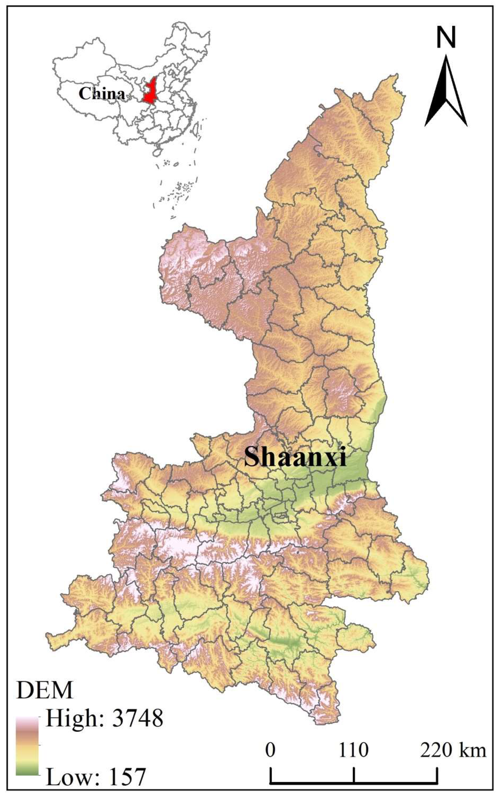
2.1. Study Area

SP is in northern-central China, spanning longitudes 105°29′ to 111°15′ E and latitudes 31°42′ to 39°35′ N (Figure 1). The province has 107 county-level administrative divisions, covering an administrative area of 205,624.3 km². Its maximum north-south distance is 878.0 km, while its maximum east-west distance is 517.3 km. The elevation ranges from 168.6 to 3771.2 m. Geographically, SP features a high terrain in the north and south, with a lower central region, showcasing a variety of landforms including plateaus, mountains, plains, and basins. The province can be divided into three distinct geographic regions: the Loess Plateau of northern SP, the Guanzhong Plain in the central area, and the Qinba Mountain area in southern SP, with areas of approximately 82,200 km², 49,400 km², and 74,000 km², respectively. SP spans three climatic zones, resulting in significant climatic variation from north to south. The Guanzhong Plain and most of northern SP are characterized by a warm temperate climate, while southern SP experiences a northern subtropical climate. The average annual temperature across the province ranges from 9 to 16 °C [33], increasing from north to south and from west to east. Precipitation is more abundant in the south and less so in the north, with average annual rainfall ranging from 340 to 1240 mm [37]. Cropland in SP accounts for approximately 20% of the total land area, with around 75% of this cropland located in northern SP and the Guanzhong Plain [30]. The per capita cropland in the province ranged from 0.06 to 0.12 hm² between 1978 and 2008 [38], which is below the national average and approaches the warning threshold of 0.053 hm² established by the Food and Agriculture Organization of the United Nations [39].

2.2. Data Source and Processing

This study selected 15 factors that comprehensively encompass both natural and anthropogenic influences on cropland change, offering a robust framework for understanding the multifaceted processes underlying CLNA. These factors are derived from reliable and readily available datasets, ensuring that the analysis is both scientifically rigorous and policy-relevant. The temporal scope of 2001–2020 was chosen to capture a period of significant socioeconomic transformation in SP, characterized by rapid urbanization, industrialization, and shifts in land use. This long timeframe enables a thorough examination of the complex interactions between socioeconomic drivers and environmental factors influencing CLNA. The topographic data utilized in this study was obtained from the Geospatial Data Cloud (http://www.gscloud.cn) with a spatial resolution of 30 m. The cropland and non-cropland dataset with a 30 m resolution is derived from the dataset published by Tu et al. (2024) [40]. Temperature and precipitation data for SP from 2001 to 2020 were collected from the National Earth System Science Data Center (https://www.geodata.cn/main/ accessed on 16 August 2023) at a spatial resolution of 1 km. Soil nutrient data, including nitrogen (N), phosphorus (P), and potassium (K) were retrieved from the Soil Science Database of the Nanjing Institute of Soil Science, Chinese Academy of Sciences (http://vdb3.soil.csdb.cn/). Economic data, including per capita GDP, county-level grain production, registered population, rural population, and per capita disposable income of rural residents in SP from 2001 to 2020 were sourced from the Shaanxi Statistical Yearbook. Population density data for SP were obtained from WorldPop (https://www.worldpop.org/). Road network density data with a spatial resolution of 1 km were derived from OpenStreetMap (https://www.openstreetmap.org).

We utilized cropland and non-cropland datasets to extract the characteristics of CLNA during the period from 2001 to 2020 using the following methods: first, the data were converted into vector format; and second, using the intersection tool in the ArcGIS platform, cropland data at time T were overlaid with non-cropland data at time T+1, enabling the identification of spatiotemporal characteristics of CLNA across different time periods.

2.3. Spatial Analysis Method of CLNA

2.3.1. Moran’s I

We utilized Moran’s I index to analyze the conversion characteristics between cropland and non-cropland areas. This index measures the degree of spatial clustering by evaluating the similarity or dissimilarity between spatial units. Moran’s I typically has two forms: Global Moran’s I (GISA) and Local Moran’s I (LISA) [7,41].

The Global Moran’s I assesses the presence of spatial autocorrelation across a region, and its formula is as follows:

$$\mathrm{G}\mathrm{I}\mathrm{S}\mathrm{A}={\displaystyle \frac{{\sum }_{\mathrm{i}=1}^{\mathrm{n}}{\sum }_{\mathrm{j}=1}^{\mathrm{n}}{\mathrm{W}}_{\mathrm{i}\mathrm{j}}({\mathrm{x}}_{\mathrm{i}}-\overline{\mathrm{x}})({\mathrm{x}}_{\mathrm{j}}-\overline{\mathrm{x}})}{{\mathrm{S}}^2{\sum }_{\mathrm{i}=1}^{\mathrm{n}}{\sum }_{\mathrm{j}=1}^{\mathrm{n}}{\mathrm{W}}_{\mathrm{i}\mathrm{j}}}}$$

where GISA is the Global Moran’s I; x_i and x_j represent the non-cropland values for counties i and j, respectively; $\overline{\mathrm{x}}$ is the mean value of non-cropland area; n denotes the number of counties; ${\mathrm{W}}_{\mathrm{i}\mathrm{j}}$ is the spatial weight matrix; where ${\mathrm{W}}_{\mathrm{i}\mathrm{j}}=1$ if counties i and j are adjacent, otherwise, ${\mathrm{W}}_{\mathrm{i}\mathrm{j}}=0$; S² is the sample variance. The value range of GISA is [−1, 1]. When GISA > 0 (closer to 1), it indicates a positive spatial correlation in CLNA. When GISA < 0 (closer to −1), it suggests a negative spatial correlation. If GISA approaches 0, the distribution of CLNA is random.

Since Global Moran’s I provides an overall measure of spatial autocorrelation, it cannot reveal specific spatial relationships between individual counties. Therefore, Local Moran’s I is computed to measure spatial association at specific locations. LISA helps identify the spatial clustering pattern of CLNA at the county level within SP. The formula for LISA is as follows:

$${\mathrm{L}\mathrm{I}\mathrm{S}\mathrm{A}}_{\mathrm{i}}={\displaystyle \frac{({\mathrm{x}}_{\mathrm{i}}-\overline{\mathrm{x}})}{{\mathrm{S}}^2}}\sum _{\mathrm{j}}{\mathrm{W}}_{\mathrm{i}\mathrm{j}}({\mathrm{x}}_{\mathrm{i}}-\overline{\mathrm{x}})$$

where LISA is the Local Moran’s I for a region; a LISA > 0 indicates spatial clustering of CLNA around county i. The higher the value, the stronger the clustering effect.

A LISA < 0 indicates spatial dispersion, with stronger dispersion effects for smaller values. A LISA = 0 suggests no spatial correlation, indicating random distribution. The statistical significance of spatial autocorrelation is determined using the standardized statistic Z_GISA [42], calculated as:

$${\mathrm{Z}}_{\mathrm{G}\mathrm{I}\mathrm{S}\mathrm{A}}={\displaystyle \frac{\mathrm{G}\mathrm{I}\mathrm{S}\mathrm{A}-{\mathrm{E}}_{\mathrm{G}\mathrm{I}\mathrm{S}\mathrm{A}}}{\sqrt{{\mathrm{V}}_{\mathrm{G}\mathrm{I}\mathrm{S}\mathrm{A}}}}}$$

where E_GISA is the expected value of GISA; V_GISA is the variance of GISA; at a significance level of 0.01, ∣Z_GISA∣ ≥ 2.58 indicates significant spatial autocorrelation.

The LISA classifies spatial clustering into five types: high-high, high-low, low-high, low-low, and not significant. The high-high type refers to areas where both the region itself and its neighboring regions are high-value areas, indicating a clustering of high-value data points in space. The high-low type reveals a spatial structure with high-value areas adjacent to low-value areas, suggesting a spatial structure characterized by a relative imbalance between high-value and low-value zones. The low-high type shows low-value areas surrounded by high-value areas, also reflecting an imbalanced spatial distribution. The low-low type represents clustering of low-value areas both in the region and its neighbors, indicating a clustering of low-value data points in space.

2.3.2. Geo-Detector

To clarify the explanatory ability of various driving factors on the trend of CLNA, we used the Geo-detector method to examine the spatial distribution of driving factors in relation to the spatial distribution of CLNA. This analysis aims to identify the explanatory capabilities of different driving factors on the CLNA in SP. The explanatory ability of a factor (or a combination of factors) regarding the target variable is typically measured using the q-statistic value [43], calculated as follows:

$$\mathrm{q}=1-{\displaystyle \frac{{\sum }_{\mathrm{h}=1}^{\mathrm{L}}{\mathrm{N}}_{\mathrm{h}}{\mathsf{\sigma }}_{\mathrm{h}}^2}{{\mathrm{N}\mathsf{\sigma }}^2}}$$

where h represents the number of influencing factors; L denotes the classification (or hierarchy) of the driving factors; ${\mathsf{\sigma }}_{\mathrm{h}}^2$ and σ² are the variances at hierarchy h and for the entire region, respectively; N_h and N are the number of evaluation units at a specific level and across the entire region, respectively. The range of q is [0, 1]. A value closer to 1 indicates a more pronounced spatial variability of the target variable y. If the stratification is generated by the independent variable X, a higher q value suggests a stronger explanatory power of X over the attribute Y, and conversely, a lower q value indicates weaker explanatory power. Specifically, q = 1 implies that variable Y is completely determined by factor X, while q = 0 suggests no correlation between factor X and variable Y. Additionally, we examined whether the interactions among different factors (X_i, X_j, …, X_n) would enhance or diminish their explanatory power regarding the dependent variable Y. Through pairwise assessments of the factors, we first calculated the q-values for X_i and X_j with respect to Y, denoted as q(X_i) and q(X_j). Subsequently, we determined the q-value of the intersection of X_i and X_j, represented as q(X_i∩X_j). Finally, we conducted a comparative analysis of q(X_i), q(X_j), and q(X_i∩X_j).

2.3.3. Model Selection and Evaluation

To effectively assess the contributions of different driving factors to CLNA, we first employed four commonly used models: Random Forest (RF) [44], XGBoost algorithm [45], LightGBM [46], and Ordinary Least Squares (OLS) [47] to simulate CLNA in SP. The 15 driving factors were selected as explanatory variables, including temperature (X1), precipitation (X2), population density (X3), elevation (X4), slope (X5), slope length (X6), road network density (X7), GDP (X8), registered population (X9), grain yield (X10), nutrient N (X11), nutrient P (X12), nutrient K (X13), rural population (X14), and per capita disposable income (X15). CLNA is set as the dependent variable. The parameters of these models were optimized using grid search and cross-validation. For example, in the RF model, we modified the number of trees (n_estimators), the maximum depth of each tree (max_depth), and the minimum number of samples required to split an internal node (min_samples_split). Similarly, for the XGBoost model, we optimized parameters such as the learning rate (eta), the maximum depth of the trees (max_depth), and the minimum sum of instance weights needed in a child node (min_child_weight). To identify the best model for CLNA predication, the relationship between the explanatory variables and the dependent variable at the county level was established. Since Shaanxi Province consists of 107 counties, a total of 107 datasets were created, each containing both explanatory and dependent variables. The model randomly selected 80% of the datasets for training, while the remaining 20% were used for testing. The Determination Coefficient (R²), Root Mean Squared Error (RMSE), and Mean Absolute Error (MAE) were used to assess the ability of each model to capture the characteristics of CLNA in the study area [48], ultimately selecting the most appropriate model.

After analyzing the statistical metrics obtained from different models, the XGBoost algorithm demonstrated the best performance. XGBoost is an ensemble machine learning algorithm implemented within a gradient boosting framework, which enhances the model’s predictive capability by incrementally adding decision trees. Each new tree is designed to correct the errors of the preceding tree by optimizing the prediction outcomes through the minimization of a loss function, such as the sum of squared residuals. Additionally, efficient parallel computation and post-pruning strategies are utilized to improve both training speed and accuracy. In this study, 15 driving factors were used to train the XGBoost algorithm. Upon completion of the training, the impacts of each factor’s weight on the CLNA were obtained. To estimate the contribution rate of each driving factor to the CLNA, the SHAP (SHapley Additive exPlanations) model was employed. SHAP is a method used for interpreting predictions from machine learning models, based on Shapley values from cooperative game theory [49]. The prediction of models are expressed as the sum of the SHAP values for each driving factor, thereby clarifying the contribution of each factor to the prediction.

3. Results

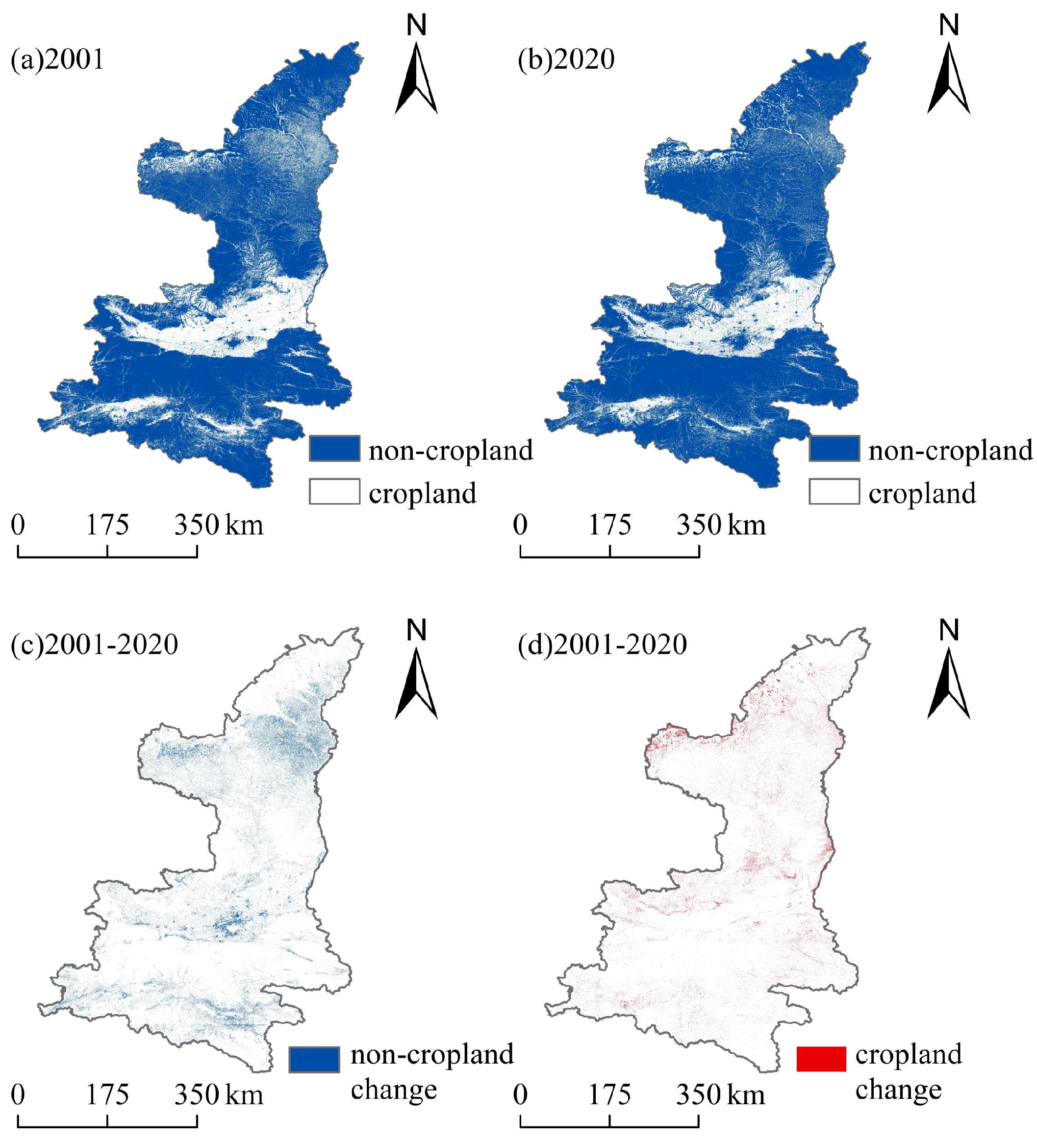
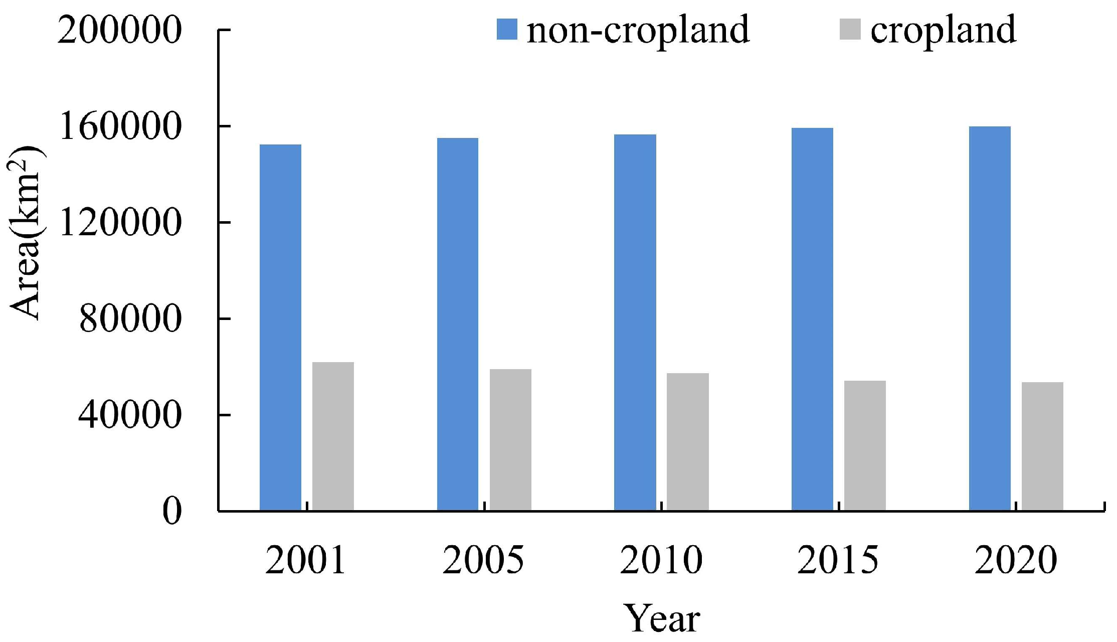
3.1. The Spatiotemporal Characteristics of CLNA in SP from 2001 to 2020

Non-cropland predominates in SP, accounting for approximately three-quarters of the total area (Figure 2a,b). Cropland in the province is primarily distributed in the central Guanzhong Plain, with a small portion in the southern region and relatively sparse and limited cropland in the northern region. In terms of area (Figure 3), the extent of non-cropland has shown a slight upward trend, increasing from 152,367.2 km² in 2001 to 159,873.6 km² in 2020, with an increasing magnitude of 7506.4 km², which accounts for 3.6% of the total area of SP. In contrast, the area of cropland exhibited a slight decline, decreasing from 53,432.8 km² in 2001 to 45,926.4 km² in 2020.

At the county level, the CLNA varied across different regions of SP (Figure 4). The northern region experienced a more significant non-agriculturalization, followed by the southern region, while the central region had the least non-agriculturalization. From 2001 onward, every five years, approximately 200–700 km² of cropland in the northern region, 100–200 km² in the southern region, and less than 100 km² in the central region were converted to non-cropland. From 2001 to 2020, a total of approximately 17,200.8 km² of cropland was converted, accounting for 8.4% of the province’s total area (Figure 5). During this period, the largest conversion occurred between 2010 and 2015, with 7616.4 km² converted; the second largest conversion took place from 2001 to 2005, with 6911.6 km² converted, while the CLNA from 2015 to 2020 was comparatively smaller, with only 5160.5 km² converted.

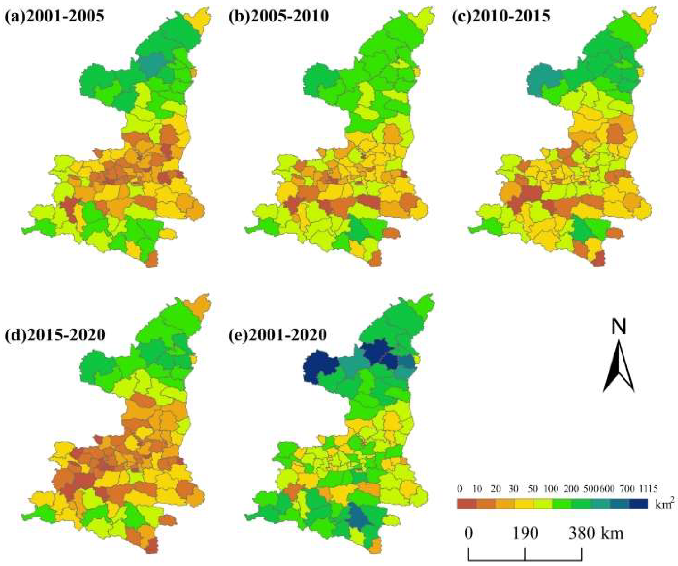
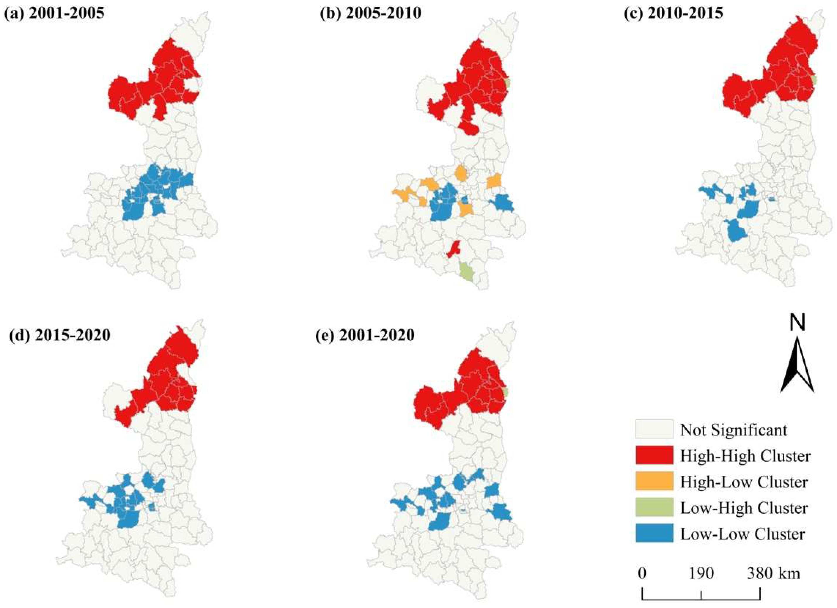
3.2. Spatial Aggregation Characteristics of CLNA in SP from 2001 to 2020

Table 1. Global Moran’s I of CLNA in SP from 2001 to 2020.

Period	Z	p	Moran’s I
2001–2005	9.92	0.00	0.58
2005–2010	7.14	0.00	0.43
2010–2015	8.85	0.00	0.52
2015–2020	8.01	0.00	0.43
2001–2020	8.96	0.00	0.54

presents the GISA indices for CLNA in SP at different stages. The GISA for all periods was greater than 0, with z-values exceeding 2.58 and p-values less than 0.01, indicating that CLNA in SP exhibits a spatially clustered distribution. The GISA from 2001 to 2020 is 0.54, suggesting a significant spatial clustering of CLNA in SP. In terms of specific periods, the GISA indices for 2001–2005 and 2010–2015 were both greater than 0.5, indicating that the spatial clustering of CLNA was particularly prominent during these two periods. The clustering types of CLNA during different time periods are illustrated in Figure 6. In the northern region of SP, the predominant clustering type was high-high cluster, with this aggregation being most evident between 2010 and 2015. This suggests that the high-value areas of CLNA in northern SP were clustered together in a continuous spatial pattern. In contrast, the central region of the SP primarily exhibits a low-low aggregation pattern, which became increasingly dispersed in the later stages of the study period, indicating that low levels of CLNA in the Guanzhong Plain of central SP were concentrated, and that this clustering pattern weakened over time.

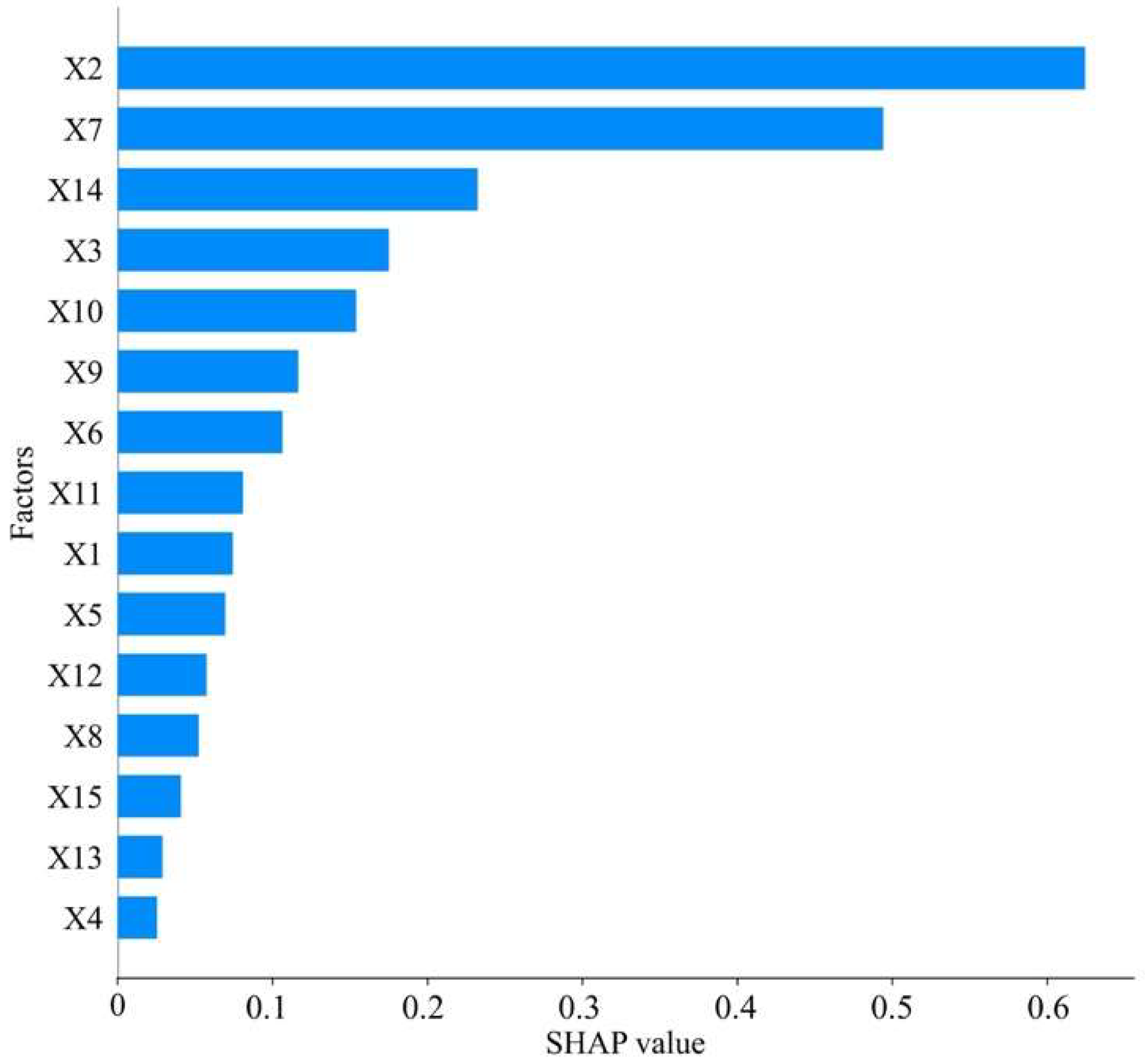
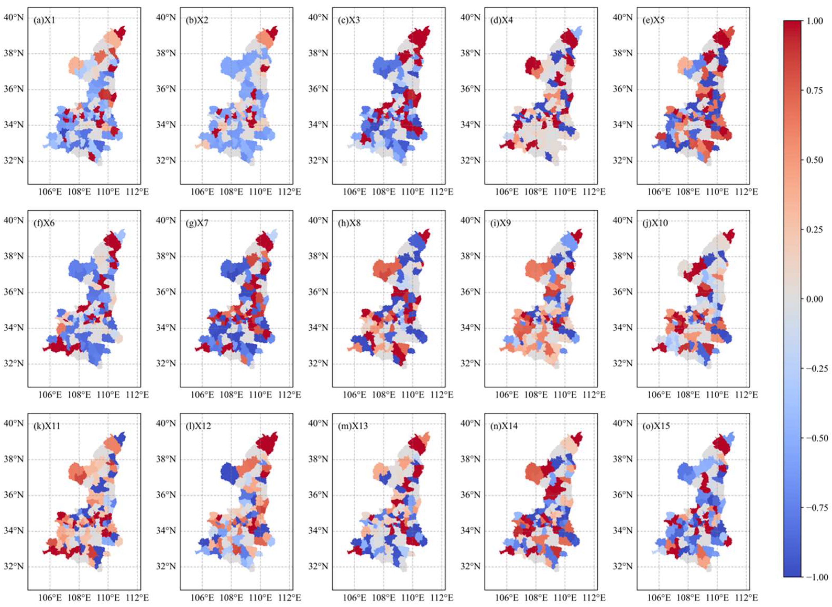
3.3. The Explanatory Power and Contribution of Different Driving Factors on CLNA

To determine the optimal model for analyzing the driving mechanisms of CLNA, we divided the driving factor dataset into training and testing phases to evaluate the prediction performance (

Table 2. Evaluation and validation of the prediction model for CLNA.

	Train_R2	Train_RMSE	Train_MAE	Test_R2	Test_RMSE	Test_MAE
RF	0.79	0.08	0.05	0.59	0.20	0.12
XGboost	0.84	0.09	0.05	0.65	0.07	0.09
LightBGM	0.81	0.10	0.06	0.59	0.11	0.08
OLS	0.26	0.18	0.13

). During the training phase, the OLS model exhibited the lowest R² value of 0.26, which did not meet the performance standards. In contrast, the R² values of the other three models were all above 0.79. The RMSE and MAE values for these models ranged from 0.08 to 0.10 and 0.05 to 0.06, respectively, both falling within acceptable ranges. In the testing phase, the R² values for the three models (excluding OLS) were all above 0.59, with RMSE and MAE ranging from 0.07 to 0.20 and 0.08 to 0.12, respectively, both still within acceptable limits. However, the XGBoost model demonstrated superior performance and was therefore chosen for further study.

Figure 7 presents the degree of explanatory power of different driving factors on CLNA in SP, based on XGBoost-SHAP. It was evident that the most significant driver of CLNA was precipitation, a natural factor, followed by road network density and population factors, which were socioeconomic factors. As a rain-fed agricultural region, precipitation has a substantial impact on farmers’ willingness to cultivate crops. For instance, a decrease in precipitation can lead to drought, which hampers crop growth and promotes CLNA. Conversely, stable precipitation fosters high crop yields, reducing the incentive for non-agriculturalization development. However, increased or extreme precipitation could prompt farmers to convert cropland to non-agricultural uses. Road network density was closely linked to CLNA in SP, mainly because improved road infrastructure provided farmers with better access to non-agricultural industries. Population growth was another key factor influencing non-agriculturalization, as increasing population pressure often leads to insufficient agricultural income to meet basic needs, pushing more people into non-agricultural industries. This phenomenon is particularly common in the Guanzhong Plain of SP. In contrast, in the more sparsely populated northern and southern regions of the province, the impact of population growth on non-agriculturalization may be less pronounced. Additionally, grain yield also played a role in non-agriculturalization; a decrease in crop yield may increase farmers’ inclination to engage in non-agricultural industries.

To further clarify the relationship between different driving factors and CLNA in various regions of SP, we visualized the SHAP values for each driving factor (Figure 8). The SHAP values for precipitation were predominantly negative, indicating that changes in precipitation are negatively correlated with CLNA in most areas of SP. Specifically, a decrease (or increase) in precipitation leads to an intensification (or reduction) of CLNA, which was especially pronounced in the northern and southern regions of the SP. Road network density had a positive effect on CLNA in the Guanzhong region and parts of northern SP, suggesting that better road networks correlate with a higher degree of CLNA. Additionally, the registered population and rural population played a positive role in CLNA across most of SP, while population density exhibited a significant positive correlation with CLNA in the central and northern regions. Grain yield showed a positive correlation with CLNA in much of SP, particularly in the central and southern regions. Although other factors, such as slope, GDP, and elevation also contributed positively to CLNA in many areas, their overall importance in driving CLNA was relatively smaller.

4. Discussion

4.1. Spatiotemporal Pattern of CLNA in SP

Cropland in SP is primarily distributed in the central Guanzhong Plain, with smaller proportions in southern SP and scattered patches in the northern region. Between 2001 and 2020, approximately 17,200.8 km² of cropland was converted to non-cropland, accounting for 8.4% of the province’s total area. Cropland conversion was most pronounced in northern SP, characterized by high-high clustering patterns driven by resource exploitation and urbanization, notably coal mining and associated infrastructure development [15]. In contrast, southern SP experienced moderate conversion, influenced by ecological conservation and adjustments in specialized agriculture [50]. The central region exhibited slower conversion, owing to the Guanzhong Plain’s competitive advantage in agricultural productivity [51]. These findings highlighted that imbalances in regional economic development and resource distribution have profoundly shaped the spatiotemporal patterns of cropland conversion. Compared to different periods, the area of CLNA in SP was evidently larger during the period of 2010–2015. On one hand, this was due to the increased development of industrial and urban construction driven by local government policies after 2010, particularly with the intensification of infrastructure projects such as highways, railways, airports, and industrial parks [52]. On the other hand, it was also a result of the implementation of stricter ecological protection and Grain for Green policies during the period of 2010–2015, especially the conversion of cropland to ecological restoration or conservation areas in mountainous and hilly regions [53]. The Moran’s I indicated a strong spatial clustering effect of CLNA in SP from 2001 to 2020; however, the clustering effect varied across different periods. The spatial clustering effect was highest during the time period of 2001–2005, driven by factors such as early economic development and the widening rural-urban gap, which propelled large-scale CLNA [54]. After 2005, this effect weakened, likely due to policy interventions and land-use optimization. However, the clustering effect strengthened again during the time period of 2010–2015, which could be attributed to local government efforts in enhancing ecological protection and vigorously implementing policies such as the Grain for Green Program (returning cropland to forest or grassland) [53]. After 2015, the Moran’s I decreased to 0.43, indicating a more dispersed spatial distribution of CLNA, although a certain degree of clustering remained.

4.2. Causes of CLNA in SP from 2001–2020

To explore the driving mechanisms of CLNA, this study selected 15 driving factors that not only directly influence agricultural productivity and land-use patterns but also capture the dynamic interactions between socioeconomic development and environmental changes. Climate factors such as temperature and precipitation shape the conditions for agricultural production. Population density and the rural population influence land demand and labor supply, while GDP and per capita disposable income reflect the connection between economic development and cropland conversion. Furthermore, topographic factors, including slope and slope length affect soil erosion and water conservation, thereby influencing the long-term sustainability of cropland. A holistic consideration of these factors contributes to a deeper understanding of the complex mechanisms driving CLNA and provides a scientific foundation for the development of sustainable land management policies. Four models, including RF, XGBoost, LightGBM, and OLS, were employed in this study. These models were selected to provide robust evaluations and offer methodological references for similar studies. Multicollinearity among 15 driving variables was assessed, revealing variance inflation factors (VIFs) exceeding 10 for several factors, with some surpassing 20, indicating significant collinearity. XGBoost was ultimately chosen for its ability to handle multicollinearity effectively by splitting nodes based on optimal features rather than all features. Although the XGBoost model showed the best performance, the R² value in the testing phase was 0.65, indicating that it explains only a portion of the variability in CLNA. This suggested that some important driving factors might be missing or that complex interactions between variables were not fully captured. These results underscored the challenges of predicting CLNA due to the complexity of the influencing factors. To improve model accuracy, further refinement was necessary, including feature expansion, data quality improvement, and optimization of the model parameterization.

We found that precipitation was the most important factor influencing the trend of CLNA in SP, which is primarily related to the precipitation distribution and recent climate changes. This finding was consistent with existing conclusions. For instance, Li et al. (2024) reported that precipitation is one of the key factors influencing changes in cultivated land [55]. Northern SP is an arid to semi-arid region with relatively low precipitation compared to other areas in the province, resulting in low crop yields. As a result, farmers often choose to transition to more economically profitable non-agricultural industries. In recent years, the frequent occurrence of extreme weather events in northern SP has increased the risks associated with agricultural production, prompting farmers to consider more economically viable sectors, such as industry and services [56]. The strong influence of precipitation on CLNA suggests that policymakers can use this information to develop adaptive strategies for agricultural and land management in areas prone to extreme weather. For instance, promoting sustainable agricultural practices or diversifying land use in regions with low and variable precipitation (northern SP) could help mitigate associated risks. We also found that road network density was positively correlated with CLNA in most regions of SP. Studies in Hubei, Jilin, Henan, and Guangdong Province have also indicated that non-agriculturalization is highly sensitive to road network development [7,57]. This was attributed to several factors. First, it was attributed to an improved road network enhancing transportation accessibility, making it easier for farmers to access markets and non-agricultural industries [58], thereby encouraging them to shift to more economically promising non-agricultural activities. Second, as road infrastructure development accelerated, urbanization processes intensified, and rural lands gradually transitioned to construction land, leading to further CLNA development. Third, the development of the road network altered rural lifestyles and consumption patterns, with more people choosing to engage in non-agricultural work, reducing the agricultural workforce and further intensifying the trend of CLNA [59]. Decision-makers can leverage this information to guide urban expansion and infrastructure development. Planning road networks in areas where non-agricultural activities are more likely to flourish can help optimize land use, ensuring efficient land allocation for agriculture, industry, and urbanization.

Consistent with previous study [16], population factors were also a significant cause of CLNA. Since 2000, the rural population in SP has shown a stable growth trend, accompanied by rapid urbanization and industrialization, leading to a marked increase in CLNA. This trend is particularly evident in the densely populated Guanzhong region, where a clear positive correlation is observed [60]. In contrast, in the sparsely populated areas of southern SP and parts of northern SP, the population density exhibited a significant negative correlation with CLNA, indicating that in areas with low population density, cropland still maintains agricultural or ecological functions [61]. These findings highlight the significant role of population dynamics in driving CLNA, particularly in densely populated areas like Guanzhong region. Rural areas with increasing populations and urbanization may need policies that balance agricultural preservation with the need for urban expansion. Conversely, sparsely populated regions where cropland still serves ecological functions may benefit from policies that promote sustainable farming and ecological preservation to prevent unnecessary land conversion. Crop yield was also related to the development of CLNA. However, compared to the factors mentioned earlier, its contribution to CLNA in SP was found to be relatively small. The relatively small but relevant role of crop yield in CLNA suggests that technological improvements in agriculture (e.g., better crop varieties, irrigation systems) in northern SP could help slow the pace of non-agriculturalization.

To better validate the reliability of the research results presented above, this study compares the results of XGBoost with those of the widely used Geo-detector (Figure 9a). The comparison showed that the ranking of q-values derived from Geo-detector was largely consistent with the ranking results obtained from XGBoost-SHAP. Although the main driving factors of CLNA in SP have been identified, we recognized that the process of CLNA did not solely result from the contribution of individual factors. The interactions between factors played a significant role and could not be overlooked. Figure 9b illustrates the impacts of factor interactions on CLNA, indicating that the interaction between any two factors was more influential than the explanatory power of individual factors. The interaction between precipitation (X2) and registered population (X9) had the strongest impact on CLNA, with a q-value of 0.79. This phenomenon has also been observed in other studies [16,55]. Moreover, the interaction between precipitation (X2) and most other factors was also pronounced, particularly the interaction with grain yield (X10), rural population (X14), and GDP (X8), with q-values above 0.66, which effectively explained the formation of spatial patterns. The above findings indicated that CLNA was the result of the combined influence of natural and socioeconomic factors. The interactions between road network density (X7) and rural population (X14), road network density (X7) and GDP (X8), as well as road network density (X7) and registered population (X9) all have q-values above 0.6. Additionally, the interactions between population density (X3), slope (X5), and most other driving factors are also notable. These results suggested that the interactions between various factors were crucial in explaining the spatial patterns of CLNA, as their combined influence surpassed that of individual factors. Key interactions, such as between precipitation and registered population, indicated a strong explanatory power. Other significant interactions involved precipitation and factors like grain yield, rural population, and GDP, as well as road network density with rural population, GDP, and registered population. These interactions underscore the importance of considering climate, population, and locational factors together, as their combined effects better explain the variations in CLNA across different regions. The results highlight the complexity and significance of factor interactions in shaping real-world outcomes, such as land use patterns.

5. Conclusions

Our results demonstrated that non-cropland in SP gradually increased, while the cropland decreased from 2001 to 2020, particularly in the northern and southern regions, where the CLNA was more pronounced. The process of CLNA in SP exhibited significant spatial clustering, with the northern region predominantly exhibiting high-high clustering, while the central region showed a low-low clustering pattern. Precipitation, road network density, and population distribution had a significant impact on CLNA, with precipitation showing a negative correlation, while road networks and population density promoted the CLNA. The interaction between different factors contributed more significantly to CLNA than individual factors, particularly the interactions of precipitation, population density, slope, and GDP, which enhanced the explanatory power of CLNA in SP. The CLNA in SP was driven by a complex combination of factors, with significant regional differences in the underlying drivers. Effective management of CLNA requires localized and comprehensive policy measures that balance food security and sustainable socioeconomic development. Future research could focus on optimizing agricultural industry layouts, integrating water-saving technology models, and conducting efficient agricultural water conservation demonstration studies in regions such as northern Shaanxi, the Wei River Loess Plateau, and the Guanzhong Plain. These efforts would provide valuable guidance for other regions facing similar challenges, helping to enhance sustainable land management and improve water-use efficiency in the context of CLNA.

References

1. Cumming, G.S.; Buerkert, A.; Hoffmann, E.M.; Schlecht, E.; von Cramon-Taubadel, S.; Tscharntke, T. Implications of agricultural transitions and urbanization for ecosystem services. Nature 2014, 515, 50–57. [Google Scholar] [CrossRef] [PubMed]
2. Viana, C.M.; Freire, D.; Abrantes, P.; Rocha, J.; Pereira, P. Agricultural land systems importance for supporting food security and sustainable development goals: A systematic review. Sci. Total Environ. 2022, 806, 150718. [Google Scholar] [CrossRef]
3. Pretty, J. Intensification for redesigned and sustainable agricultural systems. Science 2018, 362, eaav0294. [Google Scholar] [CrossRef] [PubMed]
4. Ghose, B. Food security and food self-sufficiency in China: From past to 2050. Food Energy Secur. 2014, 3, 86–95. [Google Scholar] [CrossRef]
5. Wei, Y.D.; Ye, X. Urbanization, urban land expansion and environmental change in China. Stoch. Environ. Res. Risk Assess. 2014, 28, 757–765. [Google Scholar] [CrossRef]
6. Chien, S.-S. Local farmland loss and preservation in China A perspective of quota territorialization. Land Use Policy 2015, 49, 65–74. [Google Scholar] [CrossRef]
7. Zhang, G.; Li, X.; Zhang, L.; Wei, X. Dynamics and causes of cropland non-agriculturalization in typical regions of China: An explanation Based on interpretable Machine learning. Ecol. Indic. 2024, 166, 112348. [Google Scholar] [CrossRef]
8. Chen, B.; Yao, N. Evolution characteristics of cultivated land protection policy in China based on smith policy implementation. Agriculture 2024, 14, 1194. [Google Scholar] [CrossRef]
9. Fu, B.; Li, S.; Yu, X.; Yang, P.; Yu, G.; Feng, R.; Zhuang, X. Chinese ecosystem research network: Progress and perspectives. Ecol. Complex. 2010, 7, 225–233. [Google Scholar] [CrossRef]
10. Cai, T.; Zhang, X.; Xia, F.; Zhang, Z.; Yin, J.; Wu, S. The process-mode-driving force of cropland expansion in arid regions of China based on the land use remote sensing monitoring data. Remote Sens. 2021, 13, 2949. [Google Scholar] [CrossRef]
11. Gu, C.; Hu, L.; Cook, I.G. China’s urbanization in 1949–2015: Processes and driving forces. Chin. Geogr. Sci. 2017, 27, 847–859. [Google Scholar] [CrossRef]
12. Wang, X.; Li, X. China’s agricultural land use change and its underlying drivers: A literature review. J. Geogr. Sci. 2021, 31, 1222–1242. [Google Scholar] [CrossRef]
13. Shi, K.; Yu, B.; Ma, J.; Cao, W.; Cui, Y. Impacts of slope climbing of urban expansion on global sustainable development. Innovation 2023, 4, 100529. [Google Scholar] [CrossRef] [PubMed]
14. Li, D.; He, L.; Qu, J.; Xu, X. Spatial evolution of cultivated land in the Heilongjiang Province in China from 1980 to 2015. Environ. Monit. Assess. 2022, 194, 444. [Google Scholar] [CrossRef]
15. Bryan, B.A.; Gao, L.; Ye, Y.; Sun, X.; Connor, J.D.; Crossman, N.D.; Stafford-Smith, M.; Wu, J.; He, C.; Yu, D.; et al. China’s response to a national land-system sustainability emergency. Nature 2018, 559, 193–204. [Google Scholar] [CrossRef]
16. Chen, Y.; Wang, S.; Wang, Y. Spatiotemporal evolution of cultivated land non-agriculturalization and its drivers in typical areas of southwest China from 2000 to 2020. Remote Sens. 2022, 14, 3211. [Google Scholar] [CrossRef]
17. Long, H.; Tu, S.; Ge, D.; Li, T.; Liu, Y. The allocation and management of critical resources in rural China under restructuring: Problems and prospects. J. Rural Stud. 2016, 47, 392–412. [Google Scholar] [CrossRef]
18. Zhang, B.; Sun, P.; Jiang, G.; Zhang, R.; Gao, J. Rural land use transition of mountainous areas and policy implications for land consolidation in China. J. Geogr. Sci. 2019, 29, 1713–1730. [Google Scholar] [CrossRef]
19. Zhao, H.L.; Zhou, R.L.; Zhang, T.H.; Zhao, X.Y. Effects of desertification on soil and crop growth properties in Horqin sandy cropland of Inner Mongolia, north China. Soil Tillage Res. 2006, 87, 175–185. [Google Scholar] [CrossRef]
20. Xu, X.; Tang, Q. Spatiotemporal variations in damages to cropland from agrometeorological disasters in mainland China during 1978-2018. Sci. Total Environ. 2021, 785, 147247. [Google Scholar] [CrossRef]
21. Jiang, C.; Zhang, H.; Wang, X.; Feng, Y.; Labzovskii, L. Challenging the land degradation in China’s Loess Plateau: Benefits, limitations, sustainability, and adaptive strategies of soil and water conservation. Ecol. Eng. 2019, 127, 135–150. [Google Scholar] [CrossRef]
22. Zhang, L.; Lu, D.; Li, Q.; Lu, S. Impacts of socioeconomic factors on cropland transition and its adaptation in Beijing, China. Environ. Earth Sci. 2018, 77, 575. [Google Scholar] [CrossRef]
23. Liu, X.H.; Wang, J.F.; Liu, M.L.; Meng, B. Spatial heterogeneity of the driving forces of cropland change in China. Sci. China Ser. D-Earth Sci. 2005, 48, 2231–2240. [Google Scholar] [CrossRef]
24. Xie, Y.C.; Mei, Y.; Tian, G.J.; Xing, X.R. Socio-econornic driving forces of arable land conversion: A case study of Wuxian City, China. Glob. Environ. Chang.-Hum. Policy Dimens. 2005, 15, 238–252. [Google Scholar] [CrossRef]
25. Liu, J.Y.; Liu, M.L.; Tian, H.Q.; Zhuang, D.F.; Zhang, Z.X.; Zhang, W.; Tang, X.M.; Deng, X.Z. Spatial and temporal patterns of China’s cropland during 1990–2000: An analysis based on Landsat TM data. Remote Sens. Environ. 2005, 98, 442–456. [Google Scholar] [CrossRef]
26. Poddar, I.; Roy, R. Application of GIS-based data-driven bivariate statistical models for landslide prediction: A case study of highly affected landslide prone areas of Teesta River basin. Quat. Sci. Adv. 2024, 13, 100150. [Google Scholar] [CrossRef]
27. Yang, M.; Gao, X.; Zhao, X.; Wu, P. Scale effect and spatially explicit drivers of interactions between ecosystem services—A case study from the Loess Plateau. Sci. Total Environ. 2021, 785, 147389. [Google Scholar] [CrossRef]
28. Wang, S.; Liu, Y.; Wang, W.; Zhao, G.; Liang, H. Interpretable machine learning guided by physical mechanisms reveals drivers of runoff under dynamic land use changes. J. Environ. Manag. 2024, 367, 121978. [Google Scholar] [CrossRef] [PubMed]
29. Xu, W.; Sun, T. Evaluation of rural habitat environment in under-developed areas of Western China: A case study of Northern Shaanxi. Environ. Dev. Sustain. 2022, 24, 10503–10539. [Google Scholar] [CrossRef]
30. Wei, X.; Wang, S.; Yuan, X.; Wang, X.; Zhang, B. Spatial and temporal changes and its variation of cultivated land quality in Shaanxi Province. Trans. Chin. Soc. Agric. Eng. 2018, 34, 240–248. [Google Scholar]
31. Chen, H.; Marter-Kenyon, J.; Lopez-Carr, D.; Liang, X.-y. Land cover and landscape changes in Shaanxi Province during China’s Grain for Green Program (2000–2010). Environ. Monit. Assess. 2015, 187, 644. [Google Scholar] [CrossRef] [PubMed]
32. Zhou, D.; Zhao, S.; Zhu, C. The Grain for Green Project induced land cover change in the Loess Plateau: A case study with Ansai County, Shanxi Province, China. Ecol. Indic. 2012, 23, 88–94. [Google Scholar] [CrossRef]
33. Zhang, Q.; Li, F. Correlation between land use spatial and functional transition: A case study of Shaanxi Province, China. Land Use Policy 2022, 119, 106194. [Google Scholar] [CrossRef]
34. Huang, H.; Zhou, Y.; Qian, M.; Zeng, Z. Land use transition and driving forces in Chinese Loess Plateau: A case study from Pu County, Shanxi Province. Land 2021, 10, 67. [Google Scholar] [CrossRef]
35. Jiang, S.; Chen, X.; Smettem, K.; Wang, T. Climate and land use influences on changing spatiotemporal patterns of mountain vegetation cover in southwest China. Ecol. Indic. 2020, 121, 107193. [Google Scholar] [CrossRef]
36. Li, S.; Yan, J.; Liu, X.; Wan, J. Response of vegetation restoration to climate change and human activities in Shaanxi-Gansu-Ningxia Region. J. Geogr. Sci. 2013, 23, 98–112. [Google Scholar] [CrossRef]
37. Liu, S.; Yao, S. The effect of precipitation on the Cost-Effectiveness of Sloping land conversion Program: A case study of Shaanxi Province, China. Ecol. Indic. 2021, 132, 108251. [Google Scholar] [CrossRef]
38. Li, J.; Shangguan, Z. Spatial-temporal distribution of cultivated land production capacity in Shaanxi province. Trans. Chin. Soc. Agric. Eng. 2012, 28, 239–246. [Google Scholar]
39. Qiu, J.-j.; Wang, L.-g.; Li, H.; Tang, H.-j.; Li, C.-s.; Van Ranst, E. Modeling the impacts of soil organic carbon content of croplands on crop yields in China. Agric. Sci. China 2009, 8, 464–471. [Google Scholar] [CrossRef]
40. Tu, Y.; Wu, S.; Chen, B.; Weng, Q.; Bai, Y.; Yang, J.; Yu, L.; Xu, B. A 30 m annual cropland dataset of China from 1986 to 2021. Earth Syst. Sci. Data 2024, 16, 2297–2316. [Google Scholar] [CrossRef]
41. Anselin, L. Local indicators of spatial association-LISA. Geogr. Anal. 1995, 27, 93–115. [Google Scholar] [CrossRef]
42. Anselin, L. Spatial dependence in linear regression models with an introduction to spatial econometrics. Handb. Appl. Econ. Stat. 1998, 21, 74. [Google Scholar]
43. Wang, J.-F.; Zhang, T.-L.; Fu, B.-J. A measure of spatial stratified heterogeneity. Ecol. Indic. 2016, 67, 250–256. [Google Scholar] [CrossRef]
44. Belgiu, M.; Dragut, L. Random forest in remote sensing: A review of applications and future directions. Isprs J. Photogramm. Remote Sens. 2016, 114, 24–31. [Google Scholar] [CrossRef]
45. Chen, T.; Guestrin, C. XGBoost: A scalable tree boosting system. In Proceedings of the 22nd ACM SIGKDD International Conference on Knowledge Discovery and Data Mining, San Francisco, CA, USA, 13–17 August 2016; pp. 785–794. [Google Scholar]
46. Ke, G.; Meng, Q.; Finley, T.; Wang, T.; Chen, W.; Ma, W.; Ye, Q.; Liu, T.-Y. LightGBM: A highly efficient gradient boosting decision tree. In Proceedings of the 31st Annual Conference on Neural Information Processing Systems (NIPS), Long Beach, CA, USA, 4–9 December 2017. [Google Scholar]
47. Irwin, E.G.; Geoghegan, J. Theory, data, methods: Developing spatially explicit economic models of land use change. Agric. Ecosyst. Environ. 2001, 85, 7–23. [Google Scholar] [CrossRef]
48. Wang, H.; Yang, J.; Chen, G.; Ren, C.; Zhang, J. Machine learning applications on air temperature prediction in the urban canopy layer: A critical review of 2011–2022. Urban Clim. 2023, 49, 101499. [Google Scholar] [CrossRef]
49. Han, L.; Zhao, J.; Gao, Y.; Gu, Z. Prediction and evaluation of spatial distributions of ozone and urban heat island using a machine learning modified land use regression method. Sustain. Cities Soc. 2022, 78, 103643. [Google Scholar] [CrossRef]
50. Zhu, Y.; Zhang, X.; Sun, H. Regionalization of soil and water conversation in Hanzhong City, Shaanxi Province. Bull. Soil Water Conserv. 2018, 38, 149–153,160. [Google Scholar]
51. Zhu, Z.L.; Chen, D.L. Nitrogen fertilizer use in China—Contributions to food production, impacts on the environment and best management strategies. Nutr. Cycl. Agroecosystems 2002, 63, 117–127. [Google Scholar] [CrossRef]
52. Zhang, X.; Su, B.; Yang, J.; Cong, J. Analysis of Shanxi Province’s energy consumption and intensity using input-output framework (2002–2017). Energy 2022, 250, 123786. [Google Scholar] [CrossRef]
53. Wang, T.; Gong, Z. Evaluation and analysis of water conservation function of ecosystem in Shaanxi Province in China based on “Grain for Green” Projects. Environ. Sci. Pollut. Res. 2022, 29, 83878–83896. [Google Scholar] [CrossRef] [PubMed]
54. Long, H.; Long, H. Coupling analysis of farmland and rural housing land transitions in China. In Land Use Transitions and Rural Restructuring in China; Springer: Berlin/Heidelberg, Germany, 2020; pp. 235–288. [Google Scholar]
55. Li, X.; Zhang, X.; Jin, X. Spatio-temporal characteristics and driving factors of cultivated land change in various agricultural regions of China: A detailed analysis based on county-level data. Ecol. Indic. 2024, 166, 112485. [Google Scholar] [CrossRef]
56. Yu, L.; Shi, H.; Wu, H.; Hu, X.; Ge, Y.; Yu, L.; Cao, W. The role of climate change perceptions in sustainable agricultural development: Evidence from conservation tillage technology adoption in northern China. Land 2024, 13, 705. [Google Scholar] [CrossRef]
57. Cui, X.; Zhou, T.; Xiong, X.; Xiong, J.; Zhang, J.; Jiang, Y. Farmland suitability evaluation oriented by non-agriculturalization sensitivity: A case study of Hubei Province, China. Land 2022, 11, 488. [Google Scholar] [CrossRef]
58. Njenga, P.; Davis, A. Drawing the road map to rural poverty reduction. Transp. Rev. 2003, 23, 217–241. [Google Scholar] [CrossRef]
59. Zi, C.; Qian, M.; Baozhong, G. The consumption patterns and determining factors of rural household energy: A case study of Henan Province in China. Renew. Sustain. Energy Rev. 2021, 146, 111142. [Google Scholar] [CrossRef]
60. Zhang, L.; Shi, Q.; Niu, Y.; Cao, S. Spatial distribution of population urbanlization in Guanzhong-Tianshui Economic Zone. J. Arid Land Resour. Environ. 2011, 25, 41–46. [Google Scholar]
61. DeFries, R.S.; Foley, J.A.; Asner, G.P. Land-use choices: Balancing human needs and ecosystem function. Front. Ecol. Environ. 2004, 2, 249–257. [Google Scholar] [CrossRef]
Figure 1. Geographic location and elevation characteristics of SP.
Land 14 00190 g001
Figure 2. Spatial distribution of cropland and non-cropland in SP in (a) 2001 and (b) 2020, and changes in (c) non-cropland and (d) cropland from 2001 to 2020.
Land 14 00190 g002
Figure 3. Comparison of area changes between cropland and non-cropland in SP from 2001 to 2020.
Land 14 00190 g003
Figure 4. Spatial transformation characteristics of CLNA in SP over different periods.
Land 14 00190 g004
Figure 5. Comparison of CLNA area in SP during different periods.
Land 14 00190 g005
Figure 6. LISA distribution of CLNA in SP over different periods.
Land 14 00190 g006
Figure 7. The explanatory power of different driving factors on the CLNA in SP.
Land 14 00190 g007
Figure 8. Spatial characteristics of different driving factors influencing CLNA in SP based on SHAP values. The red areas in the figure represent positive SHAP values, indicating that the driving factors in these regions contribute positively to the prediction. The blue areas represent negative SHAP values, signifying that the driving factors have a negative impact on the prediction. The larger the absolute value of the SHAP, the greater the influence of the feature on the model’s output. Lighter colors correspond to a smaller impact.
Land 14 00190 g008
Figure 9. Comparison of feature importance predicted by Geodetector and XGBoost. (a) Single-factor contributions (For Geodetector, the value of y-axis refers to the q value, while for XGBoost, it refers to the feature importance); (b) Contributions of pairwise interactions among different factors predicted by Geodetector.
Land 14 00190 g009