Abstract
Various methods for evaluating the visual quality of landscapes have been continuously studied. In the era of the rapid development of big data, methods to obtain evaluation data efficiently and accurately have received attention. However, few studies have been conducted to optimize the evaluation methods for landscape visual quality. Here, we aim to develop an evaluation model that is model fine-tuned using Scenic Beauty Evaluation (SBE) results. In elucidating the methodology, it is imperative to delve into the intricacies of refining the evaluation process. First, fine-tuning the model can be initiated with a scoring test on a small population, serving as an efficient starting point. Second, determining the optimal hyperparameter settings necessitates establishing intervals within a threshold range tailored to the characteristics of the dataset. Third, from the pool of fine-tuned models, selecting the one exhibiting optimal performance is crucial for accurately predicting the visual quality of the landscape within the study population. Lastly, through the interpolation process, discernible differences in landscape aesthetics within the core monitoring area can be visually distinguished, thereby reinforcing the reliability and practicality of the new method. In order to demonstrate the efficiency and practicality of the new method, we chose the core section of the famous Beijing–Hangzhou Grand Canal in Wujiang District, China, as a case study. The results show the following: (1) Fine-tuning the model can start with a scoring test on a small population. (2) The optimal hyperparameter setting intervals of the model need to be set in a threshold range according to different dataset characteristics. (3) The model with optimal performance is selected among the four fine-tuning models for predicting the visual quality of the landscape in the study population. (4) After the interpolation process, the differences in landscape aesthetics within the core monitoring area can be visually distinguished. We believe that the new method is efficient, accurate, and practically applicable for improving landscape visual quality evaluation.
1. Introduction
Research on assessing the visual quality of landscapes has gradually emerged since the 1960s, with early studies focusing on subjective evaluations of landscape aesthetics, concentrating on experts’ aesthetic criteria and public preferences [1]. For example, Crowe and Litton responded to the aesthetic impacts of rural landscapes and woodland landscapes, respectively [2,3]. The expert assessment model was soon adopted by government agencies in several countries, including U.S. federal agencies [4]. Daniel and Boster’s (1976) proposed Scenic Beauty Estimation (SBE) made a major breakthrough in quantifying public preferences [5]. Since then, new perspectives and dimensions are being gradually incorporated into the assessment of landscape visual quality, allowing for a more comprehensive understanding of landscape aesthetics. Examples include ecological quality and biodiversity [6,7,8], multisensory landscape experience [9,10,11], attractiveness and security [12], accessibility [13,14,15], and more.
Despite the achievements of SBE methods and other traditional techniques in landscape aesthetic assessment, they have limitations in capturing landscape diversity and dynamic character. Traditional methods tend to ignore complexity in changing urban environments and natural landscapes [16]. In addition, expert-led assessment methods face challenges of subjectivity and repeatability [17,18].
In recent years, there has been a significant shift in the field of visual quality assessment. The use of big data sources such as street view images instead of traditional film photographs is becoming mainstream, an approach that captures a broader and more realistic view of the landscape and provides more comprehensive data support [19,20,21,22,23,24]. In addition, the application of convolutional neural networks (CNNs) has revolutionized the efficiency and accuracy of image aesthetic quality assessment. CNNs are able to not only process large amounts of image data but also learn complex visual features to more accurately predict the aesthetic quality of an image. The application of these new techniques improves efficiency while providing new possibilities for understanding the diversity and subjectivity of landscape aesthetics.
The application of neural networks in the visual arts is evolving, with photography and painting being key areas of research [25]. For example, DiffRankBoost, based on RankBoost and support vector techniques, was proposed in 2010 to explore methods for estimating aesthetic scores at a fine-grain level [26]. Subsequently, Deep Multi-Patch Aggregation Network methods were used to solve the problem of image style, aesthetics, and quality assessment in high resolution images [27]. In the same year, new frameworks also emerged, such as methods for learning aesthetic features using convolutional networks and perceptual calibration systems for the automatic aesthetic assessment of photographic images [28,29]. Meanwhile, image segmentation models play an important role in landscape quantification studies, and convolutional neural network-based segmentation models can effectively identify and separate key visual elements in an image, providing more in-depth visual information for aesthetic assessment [30].
While these early approaches have made progress in image aesthetic quality assessment, they usually fail to fully understand and model the complexity of human perception and response to aesthetics. They struggle to accurately assess aesthetic quality in the absence of referents and have limitations in dealing with highly subjective and complex aesthetic assessments [31].
In recent years, the development of deep learning techniques, especially the application of CNNs, has opened up new possibilities for image aesthetic quality assessment. For example, the NIMA (Neural Image Assessment) model uses CNNs to predict the distribution of human perception rating numbers [32]. The PSAA algorithm for aesthetic attributes based on unsupervised learning [33], the MRACNN method [34] that utilizes multimodal information for aesthetic prediction, and natural language processing (NLP) techniques can provide additional contextual information to aid computers in understanding aesthetic value [35]. Deep neural networks are trained with real-life photos and corresponding scoring data to recognize visual features of urban street vitality for a better understanding of the development and evolution of cities [36]. Simultaneous human–machine–environment quantitative analysis techniques have been demonstrated to be useful for improving the reliability and accuracy of visual quality assessment results in linear landscapes [37]. All these methods and techniques provide new research perspectives for assessing the aesthetic quality of images.
In this study, we utilize CNNs and big data technology based on deep learning methods and related technical tools developed from 2015 to the present to improve the efficiency and accuracy of assessing the visual quality of landscapes and the aesthetic quality of images in landscape assessment, such as the identification of urban waterfront streetscape images.
In the subsequent sections, we discuss the following aspects in detail: (1) the selection of the study area and the basis for its delineation; (2) the process of fine-tuning the CNN model based on the SBE samples and the performance evaluation; (3) the prediction of the landscape quality of all the streetscapes in the study area using the fine-tuned model; and (4) the main findings of the study and the potential for the application of deep learning techniques in the discipline of landscaping.
2. Methods and Data
2.1. Study Area
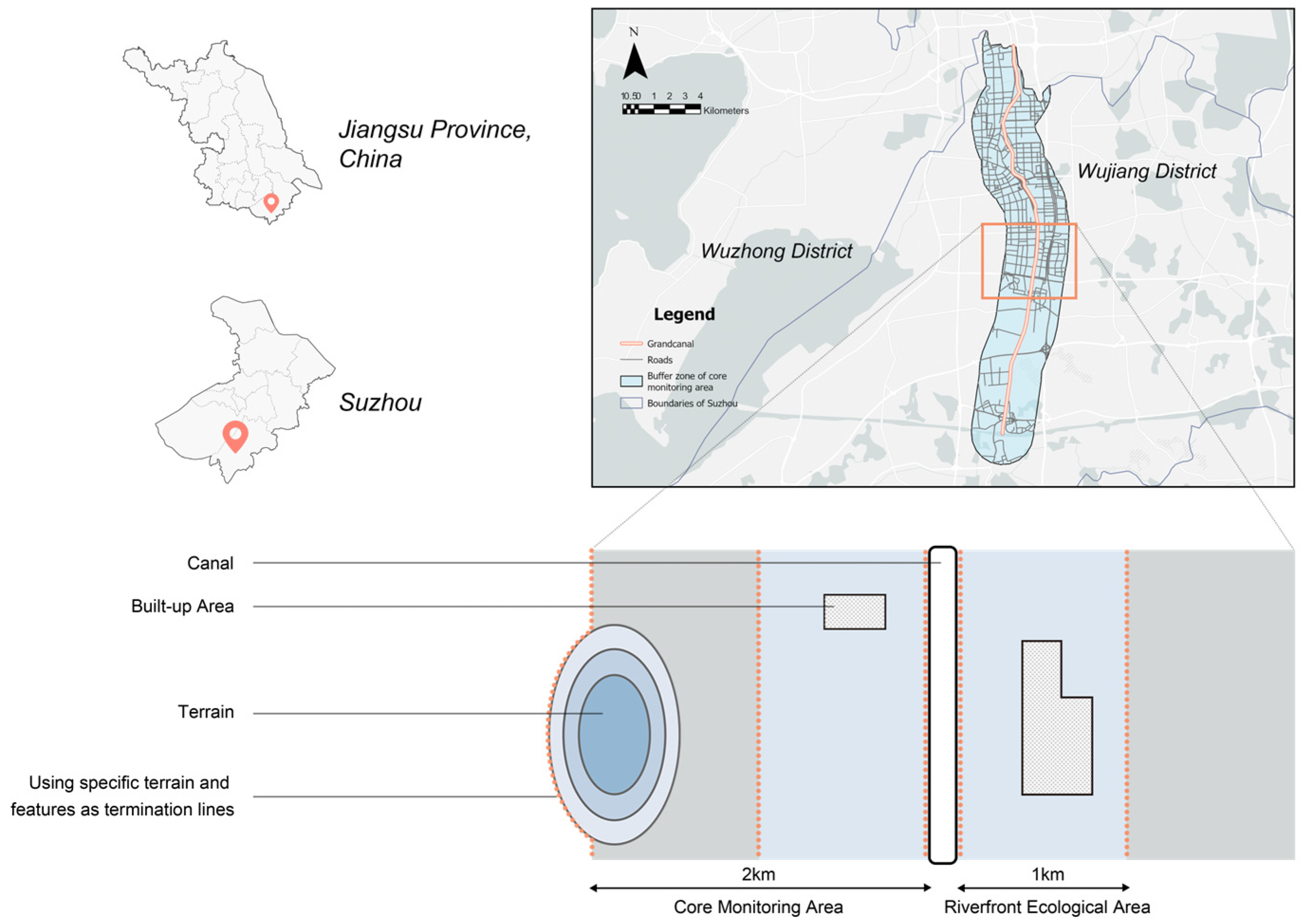
Suzhou is located in eastern China, in the center of the Yangtze River Delta and the southeast of Jiangsu Province, and it is one of the most economically active cities in China. It is an important city in the Shanghai metropolitan circle and the Suzhou–Wuxi–Changzhou metropolitan circle, as well as one of the important central cities in the Yangtze River Delta, a national high-tech industrial base and a scenic tourist city, as approved by the State Council. Due to the adjacency of the Beijing–Hangzhou Canal, the ancient city of Suzhou has become a commercial hub with nearly half of Suzhou’s freight transportation still relying on waterways. Due to the city’s history, Suzhou has the typical geographical features and diverse landscape characteristics of Jiangnan water towns. We chose Wujiang District, located in the southwest of Suzhou City, as the main study area (Figure 1), because we can observe a rich variety of landscape types in this area, including rural landscapes, urban landscapes, waterfront landscapes, and park landscapes. Here, we base our study on the categorization of the Grand Canal area in Wujiang District in local government documents. Specifically, the core monitoring area refers to the 2 km extent on each side of the main channel of the Jiangsu section of the Grand Canal. The core monitoring area includes a riverfront ecological area (i.e., in principle, in addition to the built-up area, the range of 1 km on each side of the main channel of the Jiangsu section of the Grand Canal within the core monitoring area), built-up area, and other area of the monitoring area [38]. In order to achieve the precision of this test and obtain practical research value, we selected the core monitoring area of the canal in Wujiang District as the test sample site because the canal landscape in this section is rich in visual resources and diverse in aesthetic features, which can significantly reflect the relationship between the human subjective evaluation conclusions and the results of the prediction model, and it is an ideal research object.

Figure 1.
Schematic diagram of the research area and the core monitoring area of the canal.
2.2. Methods
2.2.1. Street View Images
Streetscape imagery is widely used for neighborhood environmental quality assessment [39], street vitality [40], street safety perception [41], visual preference [42], thermal comfort perception [43], and walking route selection [44], extending to the measurement and assessment of streetscape quality [45,46,47]. With the continuous optimization of algorithms, one is able to obtain a larger range of visual fields and a finer granularity of visual information [48].
The use of street view images helps to analyze the visual quality of a canal landscape with linear characteristics. We obtained vector data of a canal water system and roads in Wujiang District from Open Street Map by using Baidu Street View (BSV) photos. Then, the road vectors in the buffer zone were extracted separately using the cropping tool. In QGIS 3.22.11, the “Points along geometry” tool was used to generate vertices on the roads at 100 m intervals [49], and these vertices’ coordinates were the acquisition coordinates of the Street View images. The original images acquired through the API are 360° panoramic images. In order to facilitate the subsequent fine-tuning of the model, we split the panoramic image obtained from a single acquisition coordinate into four sheets, which show the 90° viewpoints in the four directions of east, south, west, and north. Each image has a size of 480 × 320 pixels and a color depth of 24 bit. Finally, we import the acquisition coordinates into the Application programming interface of Baidu Street View photos to acquire Street View images in bulk. Since some image points are remote, the Baidu acquisition vehicle did not drive to them, so there are no photos. A total of 5097 acquisition coordinates were generated, and 16908 valid street view images were acquired in a batch, with an acquisition efficiency of 82.93%. This provides sufficient data support for the follow-up to model fine-tuning and analysis.
2.2.2. Landscape Beauty Assessment
The beauty degree assessment method proposed by Daniel and Boster (1976) [5] is a representative method in the theoretical framework of the psychophysical school of thought based on public appraisal with high reliability and sensitivity [50]. The method has been widely used in subjective assessment studies of landscape aesthetics because of its ability to reflect the combined opinions of diverse multi-numeric interest groups [51] and its high applicability. This study employs the universally recognized 7 point Likert scale to quantify respondents’ visual perceptions of canal landscape photographs. The model is given by Equation (1):
is the standardized rating value of the jth rater for the ith landscape, is the rating value of the jth rater for the ith landscape, is the mean of the jth rater’s ratings for all landscapes, is the standard deviation of the jth rater’s ratings for the same landscape, is the scenic beauty value for the ith landscape, and is the number of valid raters for the ith landscape.
To facilitate the testing of landscape beauty assessment for the three sub-area types within the core monitoring area, we quantified the ratio of each sub-area to the total area of the monitoring area of 105.71 square kilometers [38] as 3:5:2. The area of riverfront ecological space is 27.6 square kilometers (26.11%), the area of built-up area is 55.24 square kilometers (52.26%), and the area of the monitoring area is 22.87 square kilometers (21.63%). We randomly selected 30, 50, and 20 test images proportionally, totaling 100 images. To ensure the accuracy and recall rate of the questionnaire test, we used both online and offline methods to obtain the questionnaire results and set the time for testers to view each image to 7 s [5].
2.2.3. Convolutional Neural Network Fine-Tuning
We chose Neural Image Assessment (NIMA) as the experimental model, a mainstream neural convolutional network for image aesthetic quality assessment with the advantage of achieving a high correlation of predicted population ratings of test images in a concise architecture, which has significant advantages in prediction methods [32]. To meet the needs of this study, we used MobileNet V2 as the baseline convolutional neural network and fine-tuned it. Compared to VGG16, which has about 130 million parameters, MobileNet V2 uses only about one-forty-fifth of the number of parameters (3.22 million), but it is able to achieve about 82.98% of the performance of VGG16 [32,52].
Fine-tuning a convolutional neural network requires the use of a specific dataset. We divide the dataset into two parts: the image dataset and the score dataset. The image dataset contains the SBE-evaluated street photos, along with the photo IDs and the collected latitude and longitude coordinates; the score dataset contains the mean rank and standard deviation of the SBE evaluation results. After merging these datasets, they are divided into training, validation, and test sets in the proportions of 75%, 15%, and 10%.
After loading the pre-trained NIMA model and augmented training dataset in Matlab 2022b, the MobileNet V2 network is modified, and the training parameters are set. The main parameters affecting the performance of the model are batch size, learning rate, and epoch, respectively. The batch size is directly related to the training speed, and a larger batch size can accelerate the training speed. However, either too large or too small a batch size can negatively affect the results. Too large a batch size can cause the model to be overly dependent on a few samples in the dataset, which reduces the model’s generalization ability; too small a batch size introduces more noise, leading to an unstable training process [53]. Learning rate is one way to adjust the input weights of a neural network. For MobileNet V2, the fine-tuning learning rate is usually between 1 × 10⁻⁵ and 1 × 10⁻³. The number of iteration rounds is the number of times the training dataset passes through the network intact and returns. Pre-trained models usually have good feature extraction capabilities and thus do not require too many iteration rounds [54].
After the fine-tuning is completed, the performance of the model needs to be evaluated. The metrics used in this study are Earth Mover’s Distance (EMD), Binary Classification Accuracy (BCA), Mean Linear Correlation Coefficient (meanLCC), and Mean Spearman’s Rank Correlation Coefficient (meanSRCC). The value of EMD indicates the closeness of the prediction to the true rating distribution, and the closer the value of EMD is to 0, the closer the model is to the true rating distribution [55]. Binary Classification Accuracy is a metric used for binary classification model performance and indicates the proportion of samples correctly classified by the model. It takes values in the range of [0, 1], where 0 indicates that the model is completely wrong and 1 indicates that the model is completely correct [56]. meanLCC is used to measure the linear correlation performance of image quality evaluation models. It measures the degree of fit of the assessment model to human subjective ratings by calculating the linear correlation coefficient between the predicted values of the assessment model and the subjective ratings of the test population. The closer the value of meanLCC is to 1, the higher the linear correlation between the model and the ratings of the test population. meanSRCC is used to measure the hierarchical correlation performance of the image quality evaluation model. It measures the ranking consistency of the assessment model for human subjective ratings by calculating the Spearman rank correlation coefficient between the predicted values of the assessment model and the subjective ratings of the test population. The closer the value of meanSRCC is to 1, the higher the ranking consistency between the model and the ratings of the test population [57,58].
3. Results
3.1. Results of SBE Evaluation
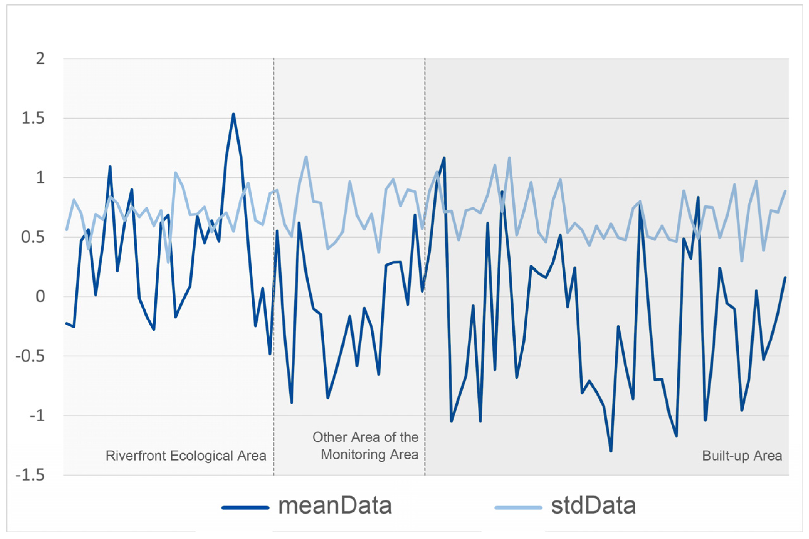
In order to obtain objective and comprehensive test data, a combination of online and offline research methods were used. A questionnaire was presented to the respondents in a compact, specific, and highly contextualized manner [59]. The online research was conducted between 14 April 2023 and 28 April 2023 using the questionnaire star program to obtain data. The offline questionnaire was conducted by the team at parks along the canal in Wujiang District, Suzhou City. The parks were Canal Ancient Slender Road Park, Canal Culture Park, and Sanliqiao Ecological Park. The research time was 22 April 2023, 12:00~17:00, and the weather was cloudy. In order to ensure that the respondents had enough time to think and make judgments, we set the display time of each test picture to 7 s, and the testers could not flip to the next test picture in advance. A total of 128 questionnaires were recovered from this test, and after eliminating invalid questionnaires filled in randomly (such as filling in only one star for all questions), a total of 100 valid questionnaires were obtained, with an effective rate of 78.13%. To reflect the principle of fairness, the respondents involved different social groups, with differences mainly in occupation, age group, and familiarity with the study area [60,61]. Meanwhile, we used SPSS to test the reliability of the questionnaire results, and the Cronbach’s α coefficient value was 0.866, which indicates that the questionnaire results are highly reliable [62] (Table 1). The inflection point of each fold in the figure represents the SBE score for a particular streetscape. The vertical axis shows the mean SBE score and standard deviation for each streetscape ID. The mean score reflects the degree to which the streetscape is perceived to be aesthetically pleasing, while the standard deviation reflects the consistency of the ratings or the diversity of opinions, with larger standard deviations indicating greater differences in opinion among evaluators [5] (Figure 2).

Table 1.
Reliability test of questionnaire results.

Figure 2.
Presentation of the results of the questionnaire survey.
Within the riparian ecological space, we observed a high fluctuation in the average SBE score curve. This is formed due to the strong visual attraction generated by landscape visual attraction elements such as the watershed, vegetation, and topography. The standard deviation of the high points reflects the subjective variability in the respondents’ evaluation of the aesthetic quality of the landscape [63]. The other areas of the monitoring zone have lower mean score values than the riverfront ecological space, with significant fluctuations. This indicates that there is a large difference in the visual favoritism of the streetscape within the area by different testers. This indicates that the richness of landscape elements within the area is high. In particular, urban streetscapes with diverse vegetation species have higher mean score values, whereas those in the outskirts of the city will have lower mean score values due to the lack of diverse vegetation species [64]. Within built-up areas, the fluctuations in mean score values increased significantly, reflecting the increased diversity of visual landscape elements within built-up areas and their compatibility with the surrounding environment, such as architectural style, scale, color, and materials [65]. The standard deviation values also showed large fluctuations, reflecting the low consistency of streetscape aesthetics scores in built-up areas. This may be due to the fact that people’s evaluations of the aesthetics of urban environments are more subjective and more likely to be influenced by personal aesthetic preferences [66].
3.2. Model Parameter Exploration Results
The main purpose of model parameter exploration when fine-tuning convolutional neural networks is to improve the performance and adaptability of CNNs [67]. We use grids that have already been trained on other datasets for continued training, which can be more efficient than starting with random weights. In order not to change the weights excessively, we assume that the existing model performs well on the new dataset and can reduce the learning rate. Reducing the learning rate helps the model to adapt to the new dataset in small steps up to the point of retaining the already learned features [68].
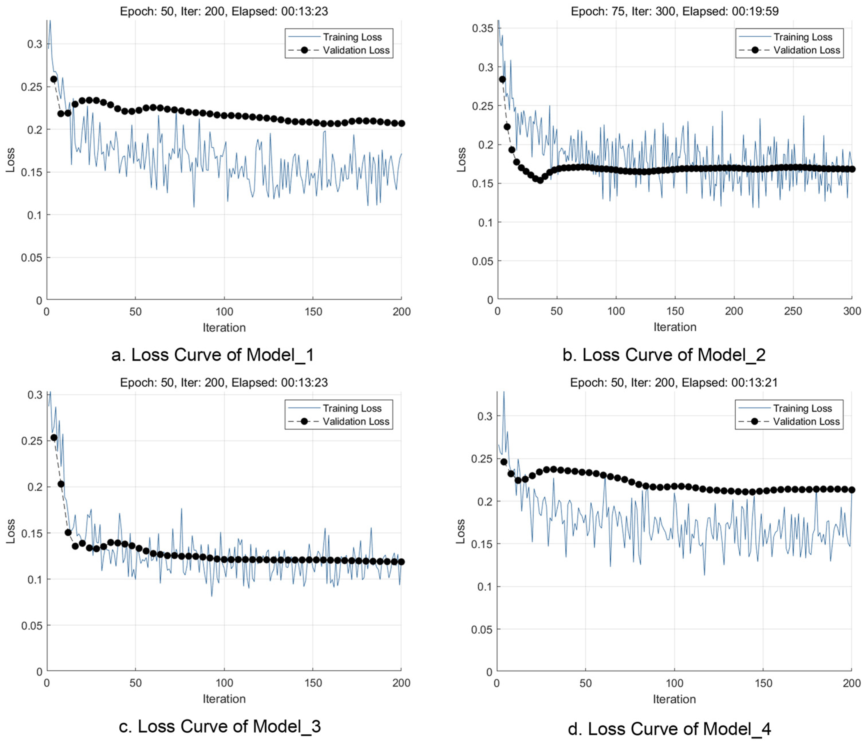
Model parameter exploration is divided into two main steps. First, the batch size of the parameters is determined. Small batch sizes provide better quality training stability and generalization performance by allowing the model to make more noisy updates during training. Large batch sizes provide fewer noisy updates and stable gradients during model training and can lead to fast but low-quality generalization [69]. To ensure that the model has good generalization ability, a batch size of 16 for this study was determined after integrating the morphology of the validation curves. Next, two sets of variables were explored, the learning rate and the number of iteration rounds. We first restrict the learning rate to 1 × 10⁻⁵ and explore the sets of iteration rounds 25, 50, 75, 100, 125, and 150. The results show that when the number of iteration rounds is less than 50, the loss curve of the model does not realize smooth convergence, and there is still a more obvious downward trend; when the number of iteration rounds is greater than 75, the loss curve of the model has completed convergence and the subsequent changes are small, and even the phenomenon of overfitting is absent; thus, 50 and 75 are the parameter values of iteration rounds for the present study. Finally, we tested all the learning rates from 1 × 10⁻⁴ to 1 × 10⁻³ at intervals of 1 × 10⁻⁴ under the conditions of 50 and 75 iteration rounds, =and the results show that the model performance is best in the interval of [5 × 10⁻⁴, 1 × 10⁻³] (Figure 3) (Table 2).
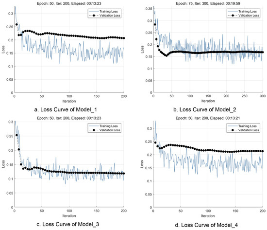
Figure 3.
Model loss curves during training.
Table 2.
Information on the four best-performing models.
3.3. Results of Model Performance Evaluation
In order to fully reflect the performance of the model, we chose two correlation indices, Pearson and Spearman, to correlate the subjective evaluations of respondents with the model in the dataset [70]. In the Pearson correlation coefficients report, the average scores of Model_1, Model_2, Model_3, and Model_4 with the average scores of the human evaluation data (meanData_0) Pearson correlation coefficients were 0.541, 0.544, 0.601, and 0.368, respectively, and all of the correlation coefficients were at the 1% level of significance (p-value < 0.001) (Table 3). This indicates that there is a moderate to strong positive correlation between the mean scores of the four models and the mean human scores, with Model_3 having the strongest correlation with the human ratings. The correlation coefficients between Model_1, Model_2, Model_3, and Model_4 show the similarity of their respective evaluation criteria. For example, Model_1 and Model_2 have a correlation of 0.622, while Model_3 and Model_4 have a correlation of 0.412, which suggests that the degree of similarity between the models internally is not high.
Table 3.
Pearson correlation test for pre-selected models.
In the Spearman mean score correlation coefficients report, the Spearman correlation coefficients of Model_1, Model_2, Model_3, and Model_4 with the human evaluation data were 0.574, 0.634, 0.661, and 0.413, respectively, and were also significant at the 1% significance level (p-value < 0.001) (Table 4). The positive correlation between model evaluation and respondent evaluation is further emphasized, with Model_3 in particular showing the strongest correlation.
Table 4.
Spearman correlation test for pre-selected models.
From the standard deviation correlation coefficients reported, it was found that the standard deviation of Model_1 showed a negative correlation with the standard deviation of the human evaluation data in Pearson’s test (−0.201) but was stronger in Spearman’s test (−0.219), both being significant at the 5% level of significance (Table 3 and Table 4). The standard deviation correlations between the Human Evaluation data and the Model Evaluation data show the extent to which they vary in consistency. For example, the correlation between human evaluation data and Model_3 is −0.227, indicating that the magnitude of change in Model_3 in the evaluation is not exactly the same as in the human evaluation; however, the correlation of standard deviations between the models shows a consistent change in the evaluation criteria. For example, the standard deviation correlation between Model_2 and Model_3 is 0.525, indicating that the two models are more similar in terms of changes in evaluation criteria.
Model_3 performed the best in terms of consistency with human evaluations, with a high degree of consistency between its Pearson and Spearman correlation coefficients (Table 3). Model_4 performed the worst in terms of consistency with human evaluations. The similarity of the evaluation criteria was higher between Model_1 and Model_2 and between Model_2 and Model_3. By comparison, Model_3 was found to perform close to the performance of the NIMA (MobileNet) model trained by TID2013 (0.698) and better than the NIMA (MobileNet) model (0.510) [32]. To summarize, Model_3 already has the theoretical performance to predict the distribution of streetscape beauty in the study area to a certain extent.
3.4. Visualization of Prediction Results
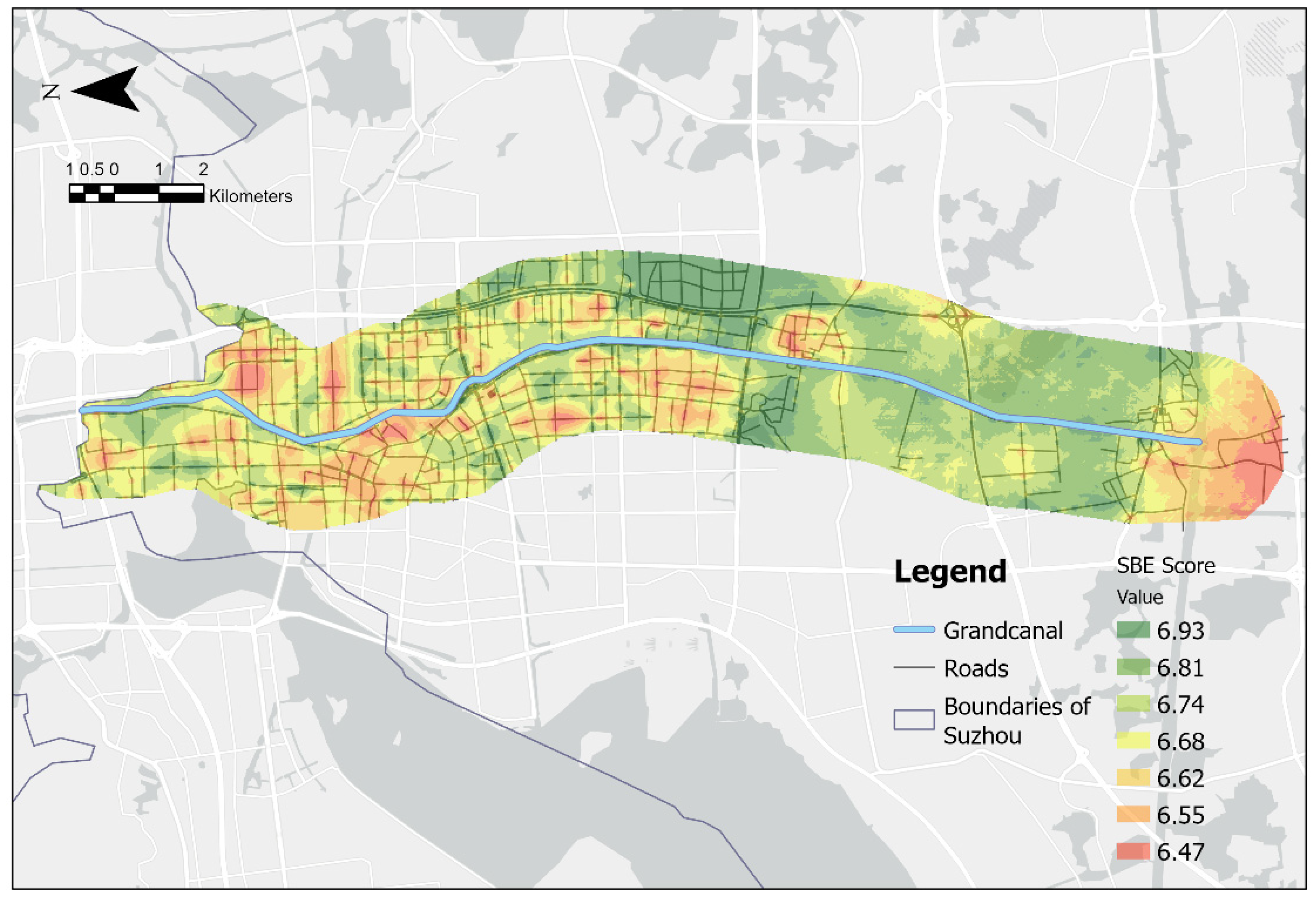
To verify the usefulness of the model, the 100 street view images used to fine-tune the model were removed. We used Model_3 to predict the remaining 16,808 street view images for human subjective evaluation and visualized the results using ArcGIS Pro 3.0.2 (Figure 4). We first mapped the prediction results containing coordinate information to form point elements on the map. Since point elements are not uniformly distributed on the map, it is necessary to rely on an interpolation process to create continuous spatial surfaces or predicted surfaces from limited point data [71]. This process covers a variety of interpolation methods including inverse distance weighting, natural neighborhood, trend, spline, and kriging. Kriging, the interpolation technique for point elements in ArcGIS Pro 3.0.2 selected for this study, is an efficient and reliable tool for spatial data analysis due to its ability to provide accurate predictions based on statistical models, its ability to optimize sampling strategies and to take into account scientific and technological trends, and its high degree of flexibility and adaptability [72]. Cross-validation is a key component to ensure the quality of kriging interpolation [73]. Bias in the model can be detected and corrected to ensure the accuracy and reliability of the interpolation results. Commonly used assessment metrics include Root Mean Square (RMS) and Average Standard Error (ASE), where the RMS is used to measure how close the predicted values are to the average measurements; the smaller the RMS, the more accurate the predicted values are, and thus the ASE value should be close to the RMS. If the opposite is true, it means that the ASE value is inaccurate [74]. These metrics help to quantify the difference between the predicted values and the actual observed values, thus assessing the performance of the model. The results of cross-validation show that the Root-Mean-Square and Average Standard Error are both at a low level (less than 0.2) and are very close to each other (Δ ≈ 0.025) (Table 5). It can be concluded that Model_3 performs well in the prediction of human subjective evaluations of street view images and that the results processed by Kriging interpolation are reliable.
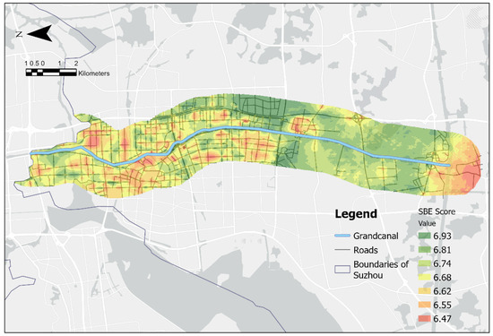
Figure 4.
SBE predictions after visualization process.
Table 5.
Summary of cross-validation report.
We statistically analyzed the landscape aesthetics of the three study areas (Table 6 and Figure 5). The built-up area had a mean of 6.67, which was the lowest among the three areas. The first and third quartiles ranged from 6.50 to 6.85; outliers were not clearly shown and there were no extreme high or low values. The standard deviation was 0.22, but due to the wide interquartile spacing, it indicated that the data were slightly more dispersed. The mean of the aesthetics of other areas in the monitoring area was about 6.72, which is tied for first place with the riverfront ecological space; the range of the first quartile and the third quartile is about 6.60 to 6.85; the outliers are not clearly shown, with some streetscapes lower than the score of 6.20, and the overall distribution of the aesthetics values is relatively centralized; the standard deviation is about 0.22, which is similar to that of the built-up area. The average beauty degree of the riverfront ecological space is 6.72, which is tied for first place with other areas in the monitoring area; the first quartile and third quartile range from 6.60 to 6.85; the outliers are not clearly shown, but some streetscapes are lower than 6.20, the lowest value is slightly higher than that of other areas in the monitoring area, and the distribution of the overall beauty degree value is relatively centralized; the standard deviation of riverfront ecological area is the smallest among the three areas, indicating that the beauty degree value of the riverfront ecological space is the most stable and consistent. Here are some examples of higher and lower ratings (Figure 6).
Table 6.
Statistics on the SBE value of each area.
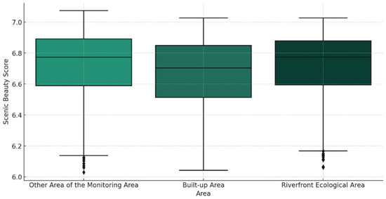
Figure 5.
Boxplot of SBE value of each area.
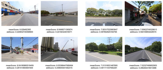
Figure 6.
Examples of higher and lower ratings.
4. Discussion
4.1. Main Findings
We found from the analysis results that there are obvious fluctuations in the landscape beauty rating values of the riverfront ecological space, other areas of the monitoring area, and the built-up area, among which the built-up area shows significant fluctuations in the beauty rating values. This indicates that there are large differences in the visual attractiveness of natural landscape features and architectural styles in different areas, which also reflects the diversity of visual landscapes and the subjectivity of evaluation groups.
By fine-tuning the pre-trained CNN and selecting appropriate hyperparameters, we were able to enhance the model’s generalization ability on small datasets. Ultimately, Model_3 is considered the optimal model for its high agreement with human evaluation on Pearson and Spearman correlation coefficients. In addition, the utility of Model_3 is validated by the prediction of a large-scale collection of street view images and the visualization of kriging interpolation in ArcGIS Pro 3.0.2. The cross-validation results show that Model_3 has a high prediction accuracy, and its root-mean-square and average standard error are at a low level, which ensures the accuracy and reliability of the interpolation results. The above metrics show that CNNs with smaller number of parameters are able to effectively learn the features of human subjective evaluations and make predictions over a wide geographic range.
According to the prediction results of Model_3, we find that the built-up area has the lowest mean value of aesthetics, while the riverfront ecological space and other areas of the monitoring area have the highest mean value of aesthetics. It indicates that landscapes with high naturalness play an important role in enhancing the visual quality of streetscape aesthetics. Overall, our study not only demonstrates the potential application of deep learning models in streetscape aesthetics evaluation but also provides an important visual aesthetics evaluation tool for urban planners.
4.2. Importance of Fine-Tuning for Performance Improvement
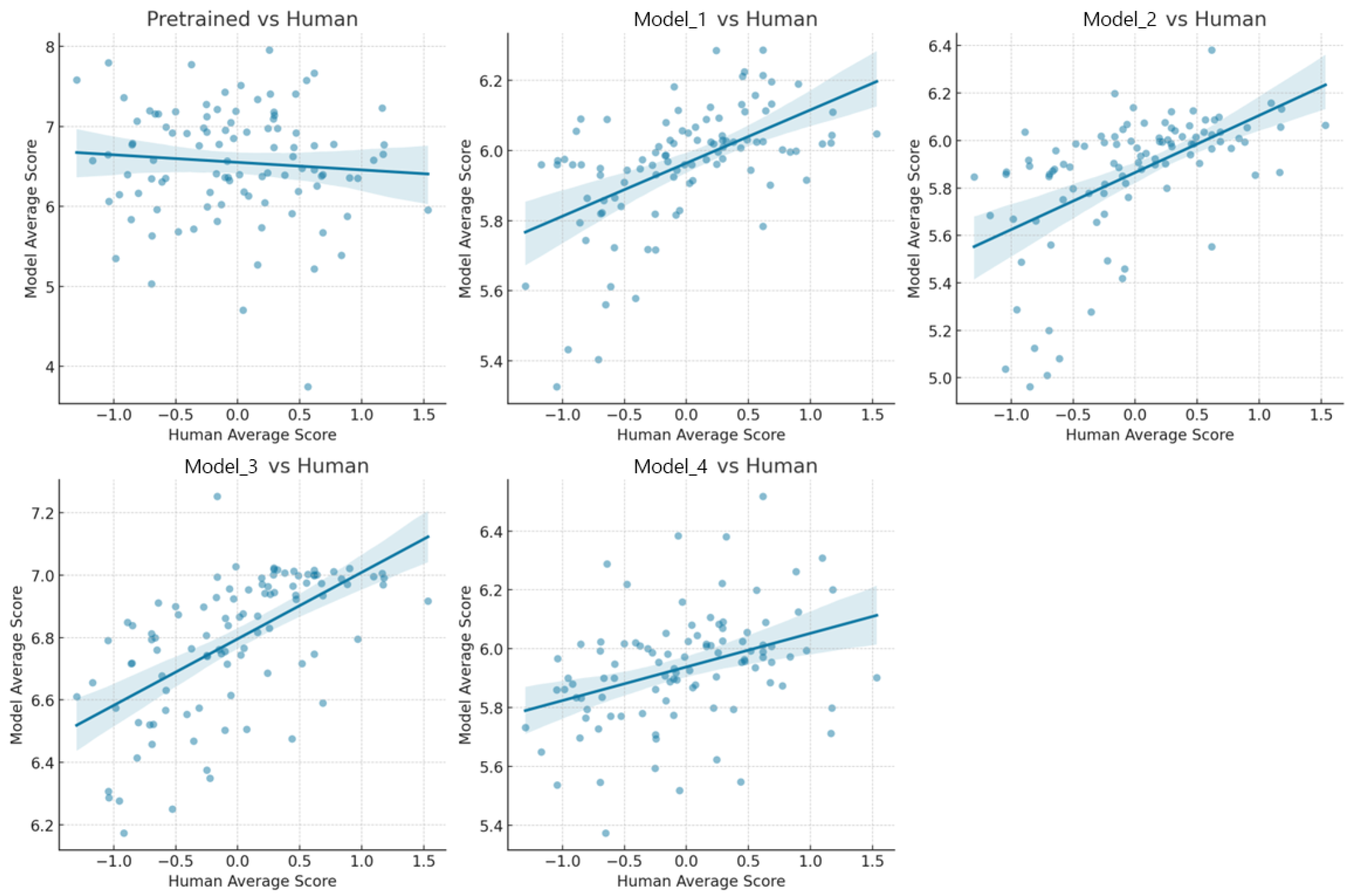
In analyzing the relationship between human ratings and each model (including one pre-trained model and four screened fine-tuned models), we found the following key phenomena. First, all the fine-tuned models showed a positive correlation with human ratings, indicating that these models were able to mimic human rating patterns to some extent. However, for the pre-trained models, the trend line showed a negative slope, suggesting a negative correlation with human ratings (Figure 7). This suggests that without fine-tuning, the model’s scoring patterns are significantly different from human scoring patterns. This finding highlights the importance of fine-tuning in machine learning, especially in scenarios where models are required to accurately understand and mimic human behavior [75]. Performance differences between fine-tuned models further reveal the possible impact of different fine-tuning strategies, highlighting the need to optimize models for specific tasks [76]. These observations not only demonstrate the potential of machine learning to mimic complex human tasks but also highlight the importance of the fine-tuning process in enabling highly specialized machine learning applications [77].
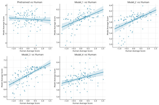
Figure 7.
Relationship between each model’s predicted score and human’s scores.
4.3. Application of Deep Learning Techniques in Landscape Disciplines
In recent years, deep learning techniques have become an important means to quantify the perception of the human living environment in the landscape discipline. In the landscape discipline, two types of deep learning models, mainly image segmentation models and natural language processing, are widely used.
4.3.1. Image Segmentation Model
The role of image segmentation models is to segment an image into different regions or objects with semantic information, which facilitates target detection and recognition tasks. In the discipline of landscape, SegNet was used to quantify the greenness, openness, and enclosure of Beijing’s hutong streetscapes to analyze the connection between the physical quality of the environment and human subjective perception [78]. The association between green visibility and residents’ mental health can be analyzed by using the green visibility indicator in separated streetscape images [79]. Image segmentation can also be used to study walking accessibility (Walkability) and street safety [80,81]
Compared to the widespread use of image segmentation models, models based on image aesthetic quality assessment have not yet received a great deal of attention in the landscape discipline at present, and the difference lies in the fact that the two yield different results: image segmentation models are mainly used to quantify landscape elements in streetscape images [82], while image aesthetic quality assessment models are mainly used to quantify the overall aesthetic quality of a streetscape image [83]. In addition, image segmentation models often do not need to be fine-tuned and can be segmented directly using the pre-trained model, while image aesthetic quality assessment models need to be fine-tuned with sample data to match experimental and practical needs [84]. Despite the generalizability of the image aesthetic quality assessment pretraining model, it does not reflect the subjective needs of a specific population [85]. The image aesthetic quality assessment model, with its prominent beauty metrics, can provide an intuitive and direct reflection of the landscape aesthetics of the study population without the need to rely on data other than street view images and human ratings.
4.3.2. Natural Language Processing Models
Natural language processing is an important branch at the intersection of computer science, artificial intelligence, and linguistics, which is dedicated to the study and development of computer systems that are capable of effectively understanding, interpreting, and modeling human language [86]. Natural language processing covers a wide range of topics including, but not limited to, speech recognition, natural language understanding, natural language generation, machine translation, and sentiment analysis. Among them, sentiment analysis is the main direction of landscape disciplines using natural language processing models, usually using social media comments as research samples, by analyzing the sentiment polarity (positive or negative labels) of the comments and identifying the positive and negative sentiment parts of the venues by using the sentiment analysis technique based on the EASYDL deep learning platform [87] for correlation analysis with other variables [88]. Sentiment analysis can also be used to identify urban park attributes associated with positive emotions, finding that visitors to different types of urban parks have different levels of positive emotions [89]. Recently, scholars have begun to combine sentiment analysis techniques with street scene image segmentation techniques. Coupling remote sensing imagery, streetscape images, social media comments, and PPGIS platform data is advocated to assist informal green space identification in the context of urban renewal [90].
Natural language processing (NLP) models and image aesthetic quality assessment models differ significantly in their core purposes, with natural language processing models focusing on interpreting and generating human language [91], while image aesthetic quality assessment models are dedicated to quantifying the overall aesthetic quality of images. However, the two exhibit certain similarities when dealing with complex data: methodologically, natural language processing models usually require a large amount of linguistic data for training in order to understand and model different linguistic structures and meanings, similar to image aesthetic quality assessment models that require a large number of images and related aesthetic scores to train their judgment criteria [92]. Furthermore, similar to image aesthetic quality assessment models, natural language processing models face the challenge of needing to adapt to specific application scenarios, such as parsing and generating text within a specific scenic area or in a specific cultural context [93]. However, despite the ability of NLP models to understand and reflect the emotion or style of a text in certain situations, this ability is not always a complete substitute for subjective human judgments, similar to the limitations of image aesthetic quality assessment models in evaluating the aesthetics of a specific population [94]. In summary, despite the different purposes for which natural language processing models and image aesthetics quality assessment models can be applied in landscape disciplines, they show some similarities in terms of dealing with highly complex datasets, the challenges they need to face, and the search for a balance between model generalizability and specific needs.
4.4. Advantages and Limitations
Compared with traditional methods, landscape assessment using convolutional neural network models has the following advantages. First, it can reduce the time and economic cost required for landscape assessment. Traditional urban landscape assessment methods require a large amount of human resources for research, while the convolutional neural network model can predict the quality of a large range of landscapes by learning a small number of samples, which effectively reduces the cost of research and improves efficiency. Second, the model is very easy to adjust. The pre-trained convolutional neural network model only needs to be fine-tuned with a small number of samples, so it is more targeted in predicting landscape quality and can meet the aesthetic needs of different landscape types and different interest groups. Finally, the current field of artificial intelligence is developing rapidly, and the field of computer vision has made rapid progress in recent years, and many excellent models have emerged, such as the image segmentation model SAM (Segment Anything Model) and the generative model DALLE-2 [95,96]. These models have strong generalization properties and do not require post-process fine-tuning by the user. Since image aesthetic quality prediction models share similar principles with these models, strong generalization performance can theoretically be achieved as well.
Of course, there are some limitations to the current use of convolutional neural networks for landscape assessment. The first is the limitation of training samples. Although the sample size required for fine-tuning the model is small, the status of the characteristics of the test population in the process of making the sample will directly affect whether the model prediction results are universally representative. This can only be achieved by having some knowledge of the demographic composition of the study area. In addition, the street view images themselves have more variables (e.g., seasons, weather), making it difficult to present the landscape in a completely objective and consistent manner. Second, there are limitations in the configuration conditions of the hardware used to analyze the data. Large models with high generalizability often need to be obtained by high-level research institutions after a long time of training on large-scale computing devices. Individual users or small-scale research institutions may find it difficult to fine-tune large models due to hardware constraints, limiting the popularity and scope of application of customized models. The above advantages and limitations make convolutional neural network modeling a promising emerging technique in the field of landscape assessment.
5. Conclusions
In conclusion, this study successfully demonstrated the feasibility of employing convolutional neural networks to emulate human subjective assessments and forecast landscape visual quality, affirming their efficacy in this domain with outcomes closely mirroring human judgments, thereby attesting to a high level of precision and robustness. Moreover, it validated the potential for achieving superior performance through model fine-tuning with a minimal dataset, broadening practical applications. By visually rendering these predictive analyses, our work fosters an intuitive grasp of varying regional landscape aesthetics, thereby enriching the understanding and practical toolbox of urban planners, landscape designers, and environmental assessment specialists. In doing so, it not only supplies these professions with innovative techniques for assessing and comprehending landscape beauty but also imparts significant insights and empirical data to the realms of computer vision and machine learning research. Ultimately, this research endeavor contributes significantly to elevating societal consciousness and appreciation concerning the value of environmental aesthetics. Our research findings furnish municipal administrations with theoretical underpinnings and hold considerable promise across multiple domains. Primarily, this technology facilitates the development of a multidimensional urban landscape aesthetics evaluation framework, encompassing both natural and man-made landscapes, as well as visual and cultural–historical values, enabling comprehensive and objective assessments tailored to the distinct characteristics of each city. Furthermore, it empowers urban administrators to conduct simulation studies on the impact of various policy interventions, such as increasing green spaces, enhancing street scenery, or preserving historical structures, on the city’s aesthetic appeal. This step is pivotal in demonstrating the potential benefits of specific changes to policymakers. Augmented by social media, policy formulation bodies can also engage citizens in the appraisal of landscape aesthetics, collecting public perceptions and preferences regarding different urban areas. This process enhances our understanding of the key elements vital for improving urban aesthetics, informing policy recommendations more attuned to popular sentiment. Lastly, we may establish a sustained monitoring and evaluation mechanism for urban landscapes, periodically assessing whether policy implementations meet expectations, if aesthetic enhancements are notable, and how these transformations influence residents’ quality of life, urban attractiveness, and tourism economy, among others. Such a system not only facilitates timely strategic adjustments but also furnishes invaluable data for subsequent research endeavors. In summary, we believe that this approach has a wide potential for application in real life and much room for development. This method brings a new interpretation to the traditional means of environmental perception, so we will continue to explore the better application of this technology in urban landscape planning and habitat improvement.
Author Contributions
Conceptualization, R.F.; Methodology, Y.C.; Software, Y.C.; Validation, Y.C.; Formal analysis, Y.C.; Investigation, Y.C.; Data curation, Y.C.; Writing—original draft, R.F. and Y.C.; Writing—review & editing, R.F. and K.P.Y.; Supervision, K.P.Y.; Project administration, R.F.; Funding acquisition, R.F. All authors have read and agreed to the published version of the manuscript.
Funding
Philosophy and Social Science in Jiangsu Province Universities: 2022SJYB0129; National Natural Sciences Foundation of China: 31700634.
Data Availability Statement
Data are contained within the article.
Conflicts of Interest
The authors declare no conflict of interest.
References
- Gobster, P.H.; Ribe, R.G.; Palmer, J.F. Themes and trends in visual assessment research: Introduction to the Landscape and Urban Planning special collection on the visual assessment of landscapes. Landsc. Urban Plan. 2019, 191, 103635. [Google Scholar] [CrossRef]
- Crowe, S.; Miller, Z. Shaping Tomorrow’s Landscape. 1964. Available online: https://cir.nii.ac.jp/crid/1130282272394986368 (accessed on 18 October 2022).
- Litton, R.B. Forest Landscape Description and Inventories: A Basis for Land Planning and Design (No. 49); Forest Service, US Department of Agriculture, Pacific Forest and Range Experiment Station: Berkeley, CA, USA, 1968.
- USDA Forest Service. National Forest Landscape Management, volume 2, chapter 1, The Visual Management System. 47: Col. Ill., Maps (Some Col.); 27 cm; USDA: Washington, DC, USA, 1974.
- Daniel, T.C. Measuring Landscape Esthetics: The Scenic Beauty Estimation Method; Department of Agriculture, Forest Service, Rocky Mountain Forest and Range Experiment Station: Fort Collins, CO, USA, 1976. [Google Scholar]
- Egoz, S.; Bowring, J.; Perkins, H.C. Tastes in tension: Form, function, and meaning in New Zealand’s farmed landscapes. Landsc. Urban Plan. 2001, 57, 177–196. [Google Scholar] [CrossRef]
- Fuller, R.A.; Irvine, K.N.; Devine-Wright, P.; Warren, P.H.; Gaston, K.J. Psychological benefits of greenspace increase with biodiversity. Biol. Lett. 2007, 3, 390–394. [Google Scholar] [CrossRef] [PubMed]
- Junker, B.; Buchecker, M. Aesthetic preferences versus ecological objectives in river restorations. Landsc. Urban Plan. 2008, 85, 141–154. [Google Scholar] [CrossRef]
- Clifford, M.A. Your Guide to Forest Bathing (Expanded Edition): Experience the Healing Power of Nature; Red Wheel: London, UK, 2021. [Google Scholar]
- Hansen, M.M.; Jones, R.; Tocchini, K. Shinrin-Yoku (Forest Bathing) and Nature Therapy: A State-of-the-Art Review. Int. J. Environ. Res. Public Health 2017, 14, 8. [Google Scholar] [CrossRef] [PubMed]
- Park, B.J.; Tsunetsugu, Y.; Kasetani, T.; Kagawa, T.; Miyazaki, Y. The physiological effects of Shinrin-yoku (taking in the forest atmosphere or forest bathing): Evidence from field experiments in 24 forests across Japan. Environ. Health Prev. Med. 2010, 15, 18–26. [Google Scholar] [CrossRef] [PubMed]
- Schroeder, H.W.; Anderson, L.M. Perception of Personal Safety in Urban Recreation Sites. J. Leis. Res. 1984, 16, 178–194. [Google Scholar] [CrossRef]
- Daniel, T.C. Whither scenic beauty? Visual landscape quality assessment in the 21st century. Landsc. Urban Plan. 2001, 54, 267–281. [Google Scholar] [CrossRef]
- Van Herzele, A.; Wiedemann, T. A monitoring tool for the provision of accessible and attractive urban green spaces. Landsc. Urban Plan. 2003, 63, 109–126. [Google Scholar] [CrossRef]
- Wright Wendel, H.E.; Zarger, R.K.; Mihelcic, J.R. Accessibility and usability: Green space preferences, perceptions, and barriers in a rapidly urbanizing city in Latin America. Landsc. Urban Plan. 2012, 107, 272–282. [Google Scholar] [CrossRef]
- Wang, R.; Zhao, J.; Liu, Z. Consensus in visual preferences: The effects of aesthetic quality and landscape types. Urban For. Urban Green. 2016, 20, 210–217. [Google Scholar] [CrossRef]
- Dupont, L.; Antrop, M.; Van Eetvelde, V. Does landscape related expertise influence the visual perception of landscape photographs? Implications for participatory landscape planning and management. Landsc. Urban Plan. 2015, 141, 68–77. [Google Scholar] [CrossRef]
- Kalivoda, O.; Vojar, J.; Skřivanová, Z.; Zahradník, D. Consensus in landscape preference judgments: The effects of landscape visual aesthetic quality and respondents’ characteristics. J. Environ. Manag. 2014, 137, 36–44. [Google Scholar] [CrossRef]
- Dunkel, A. Visualizing the perceived environment using crowdsourced photo geodata. Landsc. Urban Plan. 2015, 142, 173–186. [Google Scholar] [CrossRef]
- Li, X.; Zhang, C.; Li, W.; Ricard, R.; Meng, Q.; Zhang, W. Assessing street-level urban greenery using Google Street View and a modified green view index. Urban For. Urban Green. 2015, 14, 675–685. [Google Scholar] [CrossRef]
- Lu, Y.; Yang, Y.; Sun, G.; Gou, Z. Associations between overhead-view and eye-level urban greenness and cycling behaviors. Cities 2019, 88, 10–18. [Google Scholar] [CrossRef]
- Tieskens, K.F.; Van Zanten, B.T.; Schulp, C.J.E.; Verburg, P.H. Aesthetic appreciation of the cultural landscape through social media: An analysis of revealed preference in the Dutch river landscape. Landsc. Urban Plan. 2018, 177, 128–137. [Google Scholar] [CrossRef]
- Ye, Y.; Richards, D.; Lu, Y.; Song, X.; Zhuang, Y.; Zeng, W.; Zhong, T. Measuring daily accessed street greenery: A human-scale approach for informing better urban planning practices. Landsc. Urban Plan. 2019, 191, 103434. [Google Scholar] [CrossRef]
- Zhu, H.; Nan, X.; Yang, F.; Bao, Z. Utilizing the green view index to improve the urban street greenery index system: A statistical study using road patterns and vegetation structures as entry points. Landsc. Urban Plan. 2023, 237, 104780. [Google Scholar] [CrossRef]
- Santos, I.; Castro, L.; Rodriguez-Fernandez, N.; Torrente-Patino, A.; Carballal, A. Artificial neural networks and deep learning in the visual arts: A review. Neural Comput. Appl. 2021, 33, 121–157. [Google Scholar] [CrossRef]
- Jiang, W.; Loui, A.C.; Cerosaletti, C.D. Automatic aesthetic value assessment in photographic images. In Proceedings of the 2010 IEEE International Conference on Multimedia and Expo, Singapore, 19–23 July 2010; pp. 920–925. [Google Scholar] [CrossRef]
- Lu, X.; Lin, Z.; Shen, X.; Mech, R.; Wang, J.Z. Deep multi-patch aggregation network for image style, aesthetics, and quality estimation. In Proceedings of the IEEE International Conference on Computer Vision, Santiago, Chile, 7–13 December 2015; pp. 990–998. [Google Scholar]
- Aydın, T.O.; Smolic, A.; Gross, M. Automated Aesthetic Analysis of Photographic Images. IEEE Trans. Vis. Comput. Graph. 2015, 21, 31–42. [Google Scholar] [CrossRef]
- Kao, Y.; Wang, C.; Huang, K. Visual aesthetic quality assessment with a regression model. In Proceedings of the 2015 IEEE International Conference on Image Processing (ICIP), Quebec City, QC, Canada, 27–30 September 2015; pp. 1583–1587. [Google Scholar] [CrossRef]
- Aikoh, T.; Homma, R.; Abe, Y. Comparing conventional manual measurement of the green view index with modern automatic methods using google street view and semantic segmentation. Urban For. Urban Green. 2023, 80, 127845. [Google Scholar] [CrossRef]
- Chandler, D.M. Seven Challenges in Image Quality Assessment: Past, Present, and Future Research. Int. Sch. Res. Not. 2013, 2013, e905685. [Google Scholar] [CrossRef]
- Talebi, H.; Milanfar, P. NIMA: Neural Image Assessment. IEEE Trans. Image Process. 2018, 27, 3998–4011. [Google Scholar] [CrossRef]
- Lee, J.-T.; Lee, C.; Kim, C.-S. Property-Specific Aesthetic Assessment With Unsupervised Aesthetic Property Discovery. IEEE Access 2019, 7, 114349–114362. [Google Scholar] [CrossRef]
- Zhang, X.; Gao, X.; Lu, W.; He, L.; Li, J. Beyond Vision: A Multimodal Recurrent Attention Convolutional Neural Network for Unified Image Aesthetic Prediction Tasks. IEEE Trans. Multimed. 2021, 23, 611–623. [Google Scholar] [CrossRef]
- Wang, W.; Yang, S.; Zhang, W.; Zhang, J. Neural aesthetic image reviewer. IET Comput. Vis. 2019, 13, 749–758. [Google Scholar] [CrossRef]
- Qi, Y.; Chodron Drolma, S.; Zhang, X.; Liang, J.; Jiang, H.; Xu, J.; Ni, T. An investigation of the visual features of urban street vitality using a convolutional neural network. Geo-Spat. Inf. Sci. 2020, 23, 341–351. [Google Scholar] [CrossRef]
- Zhang, X.; Xiong, X.; Chi, M.; Yang, S.; Liu, L. Research on visual quality assessment and landscape elements influence mechanism of rural greenways. Ecol. Indic. 2024, 160, 111844. [Google Scholar] [CrossRef]
- General Office of the People’s Government of Jiangsu Province. (28 February 2021). Notice of the Provincial Government on the Issuance of Interim Measures for the Control of Land Space in the Core Monitoring Area of the Jiangsu Section of the Grand Canal. Available online: http://www.jiangsu.gov.cn/art/2021/4/7/art_46143_9745264.html (accessed on 4 February 2023).
- Larkin, A.; Gu, X.; Chen, L.; Hystad, P. Predicting perceptions of the built environment using GIS, satellite and street view image approaches. Landsc. Urban Plan. 2021, 216, 104257. [Google Scholar] [CrossRef] [PubMed]
- Wu, C.; Ye, Y.; Gao, F.; Ye, X. Using street view images to examine the association between human perceptions of locale and urban vitality in Shenzhen, China. Sustain. Cities Soc. 2023, 88, 104291. [Google Scholar] [CrossRef]
- Sainju, A.M.; Jiang, Z. Mapping road safety features from streetview imagery: A deep learning approach. ACM Trans. Data Sci. 2020, 1, 1–20. [Google Scholar] [CrossRef]
- Evans-Cowley, J.S.; Akar, G. StreetSeen visual survey tool for determining factors that make a street attractive for bicycling. Transp. Res. Rec. 2014, 2468, 19–27. [Google Scholar] [CrossRef]
- Li, Y.; Yabuki, N.; Fukuda, T. Integrating GIS, deep learning, and environmental sensors for multicriteria evaluation of urban street walkability. Landsc. Urban Plan. 2023, 230, 104603. [Google Scholar] [CrossRef]
- Chen, L.; Lu, Y.; Sheng, Q.; Ye, Y.; Wang, R.; Liu, Y. Estimating pedestrian volume using Street View images: A large-scale validation test. Comput. Environ. Urban Syst. 2020, 81, 101481. [Google Scholar] [CrossRef]
- Ki, D.; Lee, S. Analyzing the effects of Green View Index of neighborhood streets on walking time using Google Street View and deep learning. Landsc. Urban Plan. 2021, 205, 103920. [Google Scholar] [CrossRef]
- Lu, Y. Using Google Street View to investigate the association between street greenery and physical activity. Landsc. Urban Plan. 2019, 191, 103435. [Google Scholar] [CrossRef]
- Seiferling, I.; Naik, N.; Ratti, C.; Proulx, R. Green streets − Quantifying and mapping urban trees with street-level imagery and computer vision. Landsc. Urban Plan. 2017, 165, 93–101. [Google Scholar] [CrossRef]
- Ibrahim, M.R.; Haworth, J.; Cheng, T. Understanding cities with machine eyes: A review of deep computer vision in urban analytics. Cities 2020, 96, 102481. [Google Scholar] [CrossRef]
- Kim, J.H.; Lee, S.; Hipp, J.R.; Ki, D. Decoding urban landscapes: Google street view and measurement sensitivity. Comput. Environ. Urban Syst. 2021, 88, 101626. [Google Scholar] [CrossRef]
- Vodak, M.C.; Roberts, P.L.; Wellman, J.D.; Buhyoff, G.J. Scenic impacts of eastern hardwood management. For. Sci. 1985, 31, 289–301. [Google Scholar]
- Zhai, M.; Zhang, R.; Yan, H. Review on the Studies on Scenic Evaluation and Its Application in Scenic Forest Construction both at Home and Abroad. World For. Res. 2003, 6, 16–19. [Google Scholar] [CrossRef]
- Sandler, M.; Howard, A.; Zhu, M.; Zhmoginov, A.; Chen, L.-C. MobileNetV2: Inverted Residuals and Linear Bottlenecks. In Proceedings of the 2018 IEEE/CVF Conference on Computer Vision and Pattern Recognition, Salt Lake City, UT, USA, 18–23 June 2018; pp. 4510–4520. [Google Scholar] [CrossRef]
- Smith, S.L.; Le, Q.V. A Bayesian Perspective on Generalization and Stochastic Gradient Descent. arXiv 2018, arXiv:1710.06451. [Google Scholar] [CrossRef]
- Shin, H.-C.; Roth, H.R.; Gao, M.; Lu, L.; Xu, Z.; Nogues, I.; Yao, J.; Mollura, D.; Summers, R.M. Deep Convolutional Neural Networks for Computer-Aided Detection: CNN Architectures, Dataset Characteristics and Transfer Learning. IEEE Trans. Med. Imaging 2016, 35, 1285–1298. [Google Scholar] [CrossRef] [PubMed]
- Hou, L.; Yu, C.-P.; Samaras, D. Squared Earth Mover’s Distance-based Loss for Training Deep Neural Networks. arXiv 2017, arXiv:1611.05916. [Google Scholar] [CrossRef]
- Zliobaite, I. On the relation between accuracy and fairness in binary classification. arXiv 2015, arXiv:1505.05723. [Google Scholar] [CrossRef]
- Liu, Y.; Zhang, Z.; Liu, X.; Wang, L.; Xia, X. Ore image classification based on small deep learning model: Evaluation and optimization of model depth, model structure and data size. Miner. Eng. 2021, 172, 107020. [Google Scholar] [CrossRef]
- Zhang, W.; Ma, K.; Yan, J.; Deng, D.; Wang, Z. Blind Image Quality Assessment Using a Deep Bilinear Convolutional Neural Network. IEEE Trans. Circuits Syst. Video Technol. 2020, 30, 36–47. [Google Scholar] [CrossRef]
- Harris, L.; Brown, G. Mixing interview and questionnaire methods: Practical problems in aligning data. Pract. Assess. Res. Eval. 2019, 15, 1. [Google Scholar] [CrossRef]
- Dadvand, P.; Wright, J.; Martinez, D.; Basagaña, X.; McEachan, R.R.C.; Cirach, M.; Gidlow, C.J.; de Hoogh, K.; Gražulevičienė, R.; Nieuwenhuijsen, M.J. Inequality, green spaces, and pregnant women: Roles of ethnicity and individual and neighbourhood socioeconomic status. Environ. Int. 2014, 71, 101–108. [Google Scholar] [CrossRef]
- Shen, Y.; Sun, F.; Che, Y. Public green spaces and human wellbeing: Mapping the spatial inequity and mismatching status of public green space in the Central City of Shanghai. Urban For. Urban Green. 2017, 27, 59–68. [Google Scholar] [CrossRef]
- Taherdoost, H. Validity and Reliability of the Research Instrument; How to Test the Validation of a Questionnaire/Survey in a Research (10 August 2016). Available online: https://ssrn.com/abstract=3205040 (accessed on 15 May 2023).
- Hu, S.; Yue, H.; Zhou, Z. Preferences for urban stream landscapes: Opportunities to promote unmanaged riparian vegetation. Urban For. Urban Green. 2019, 38, 114–123. [Google Scholar] [CrossRef]
- Tian, Y.; Qian, J. Suburban identification based on multi-source data and landscape analysis of its construction land: A case study of Jiangsu Province, China. Habitat Int. 2021, 118, 102459. [Google Scholar] [CrossRef]
- Lindal, P.J.; Hartig, T. Architectural variation, building height, and the restorative quality of urban residential streetscapes. J. Environ. Psychol. 2013, 33, 26–36. [Google Scholar] [CrossRef]
- Zhou, L.; Li, Y.; Cheng, J.; Qin, Y.; Shen, G.; Li, B.; Yang, H.; Li, S. Understanding the aesthetic perceptions and image impressions experienced by tourists walking along tourism trails through continuous cityscapes in Macau. J. Transp. Geogr. 2023, 112, 103703. [Google Scholar] [CrossRef]
- Yin, X.; Chen, W.; Wu, X.; Yue, H. Fine-tuning and visualization of convolutional neural networks. In Proceedings of the 2017 12th IEEE Conference on Industrial Electronics and Applications (ICIEA), Siem Reap, Cambodia, 18–20 June 2017; pp. 1310–1315. [Google Scholar] [CrossRef]
- Becherer, N.; Pecarina, J.; Nykl, S.; Hopkinson, K. Improving optimization of convolutional neural networks through parameter fine-tuning. Neural Comput. Appl. 2019, 31, 3469–3479. [Google Scholar] [CrossRef]
- Kandel, I.; Castelli, M. The effect of batch size on the generalizability of the convolutional neural networks on a histopathology dataset. ICT Express 2020, 6, 312–315. [Google Scholar] [CrossRef]
- Zheng, T.; Bergin, M.H.; Hu, S.; Miller, J.; Carlson, D.E. Estimating ground-level PM2.5 using micro-satellite images by a convolutional neural network and random forest approach. Atmos. Environ. 2020, 230, 117451. [Google Scholar] [CrossRef]
- Li, J.; Heap, A.D. Spatial interpolation methods applied in the environmental sciences: A review. Environ. Model. Softw. 2014, 53, 173–189. [Google Scholar] [CrossRef]
- Oliver, M.A.; Webster, R. Kriging: A method of interpolation for geographical information systems. Int. J. Geogr. Inf. Syst. 1990, 4, 313–332. [Google Scholar] [CrossRef]
- Theodossiou, N.; Latinopoulos, P. Evaluation and optimisation of groundwater observation networks using the Kriging methodology. Environ. Model. Softw. 2006, 21, 991–1000. [Google Scholar] [CrossRef]
- Knotters, M.; Brus, D.J.; Oude Voshaar, J.H. A comparison of kriging, co-kriging and kriging combined with regression for spatial interpolation of horizon depth with censored observations. Geoderma 1995, 67, 227–246. [Google Scholar] [CrossRef]
- Gupta, J.; Pathak, S.; Kumar, G. Deep Learning (CNN) and Transfer Learning: A Review. J. Phys. Conf. Ser. 2022, 2273, 012029. [Google Scholar] [CrossRef]
- Ma, J.; Zhao, Z.; Yi, X.; Chen, J.; Hong, L.; Chi, E.H. Modeling Task Relationships in Multi-task Learning with Multi-gate Mixture-of-Experts. In Proceedings of the 24th ACM SIGKDD International Conference on Knowledge Discovery & Data Mining, London, UK, 19–23 August 2018; pp. 1930–1939. [Google Scholar] [CrossRef]
- Talukder, A.; Islam, M.; Uddin, A.; Akhter, A.; Pramanik, A.J.; Aryal, S.; Almoyad, M.A.A.; Hasan, K.F.; Moni, M.A. An efficient deep learning model to categorize brain tumor using reconstruction and fine-tuning. Expert Syst. Appl. 2023, 230, 120534. [Google Scholar] [CrossRef]
- Tang, J.; Long, Y. Measuring visual quality of street space and its temporal variation: Methodology and its application in the Hutong area in Beijing. Landsc. Urban Plan. 2019, 191, 103436. [Google Scholar] [CrossRef]
- Helbich, M.; Poppe, R.; Oberski, D.; Zeylmans van Emmichoven, M.; Schram, R. Can’t see the wood for the trees? An assessment of street view- and satellite-derived greenness measures in relation to mental health. Landsc. Urban Plan. 2021, 214, 104181. [Google Scholar] [CrossRef]
- Jeon, J.; Woo, A. Deep learning analysis of street panorama images to evaluate the streetscape walkability of neighborhoods for subsidized families in Seoul, Korea. Landsc. Urban Plan. 2023, 230, 104631. [Google Scholar] [CrossRef]
- Koo, B.W.; Guhathakurta, S.; Botchwey, N.; Hipp, A. Can good microscale pedestrian streetscapes enhance the benefits of macroscale accessible urban form? An automated audit approach using Google street view images. Landsc. Urban Plan. 2023, 237, 104816. [Google Scholar] [CrossRef]
- Suzuki, M.; Mori, J.; Maeda, T.N.; Ikeda, J. The economic value of urban landscapes in a suburban city of Tokyo, Japan: A semantic segmentation approach using Google Street View images. J. Asian Archit. Build. Eng. 2023, 22, 1110–1125. [Google Scholar] [CrossRef]
- Deng, Y.; Loy, C.C.; Tang, X. Image Aesthetic Assessment: An experimental survey. IEEE Signal Process. Mag. 2017, 34, 80–106. [Google Scholar] [CrossRef]
- Lv, P.; Fan, J.; Nie, X.; Dong, W.; Jiang, X.; Zhou, B.; Xu, M.; Xu, C. User-Guided Personalized Image Aesthetic Assessment Based on Deep Reinforcement Learning. IEEE Trans. Multimed. 2023, 25, 736–749. [Google Scholar] [CrossRef]
- Mormont, R.; Geurts, P.; Marée, R. Multi-Task Pre-Training of Deep Neural Networks for Digital Pathology. IEEE J. Biomed. Health Inform. 2021, 25, 412–421. [Google Scholar] [CrossRef] [PubMed]
- Kang, Y.; Cai, Z.; Tan, C.-W.; Huang, Q.; Liu, H. Natural language processing (NLP) in management research: A literature review. J. Manag. Anal. 2020, 7, 139–172. [Google Scholar] [CrossRef]
- Luo, J.; Lei, Z.; Hu, Y.; Wang, M.; Cao, L. Analysis of Tourists’ Sentiment Tendency in Urban Parks Based on Deep Learning: A Case Study of Tianjin Water Park. Chin. Landsc. Archit. 2021, 37, 65–70. [Google Scholar] [CrossRef]
- Shivaprasad, T.K.; Shetty, J. Sentiment analysis of product reviews: A review. In Proceedings of the 2017 International Conference on Inventive Communication and Computational Technologies (ICICCT), Coimbatore, India, 10–11 March 2017; pp. 298–301. [Google Scholar] [CrossRef]
- Kong, L.; Liu, Z.; Pan, X.; Wang, Y.; Guo, X.; Wu, J. How do different types and landscape attributes of urban parks affect visitors’ positive emotions? Landsc. Urban Plan. 2022, 226, 104482. [Google Scholar] [CrossRef]
- Liu, J.; Ettema, D.; Helbich, M. Street view environments are associated with the walking duration of pedestrians: The case of Amsterdam, the Netherlands. Landsc. Urban Plan. 2023, 235, 104752. [Google Scholar] [CrossRef]
- Sun, X.; Yang, D.; Li, X.; Zhang, T.; Meng, Y.; Qiu, H.; Wang, G.; Hovy, E.; Li, J. Interpreting Deep Learning Models in Natural Language Processing: A Review. arXiv 2021, arXiv:2110.10470. [Google Scholar] [CrossRef]
- Jiang, H.; He, P.; Chen, W.; Liu, X.; Gao, J.; Zhao, T. SMART: Robust and Efficient Fine-Tuning for Pre-trained Natural Language Models through Principled Regularized Optimization. In Proceedings of the 58th Annual Meeting of the Association for Computational Linguistics, Seattle, WA, USA, 5–10 July 2020; pp. 2177–2190. [Google Scholar] [CrossRef]
- Gu, Y.; Tinn, R.; Cheng, H.; Lucas, M.; Usuyama, N.; Liu, X.; Naumann, T.; Gao, J.; Poon, H. Domain-Specific Language Model Pretraining for Biomedical Natural Language Processing. ACM Trans. Comput. Healthc. 2021, 3, 2:1–2:23. [Google Scholar] [CrossRef]
- Khurana, D.; Koli, A.; Khatter, K.; Singh, S. Natural language processing: State of the art, current trends and challenges. Multimed. Tools Appl. 2023, 82, 3713–3744. [Google Scholar] [CrossRef]
- Gozalo-Brizuela, R.; Garrido-Merchan, E.C. ChatGPT is not all you need. A State of the Art Review of large Generative AI models. arXiv 2023, arXiv:2301.04655. [Google Scholar] [CrossRef]
- Kirillov, A.; Mintun, E.; Ravi, N.; Mao, H.; Rolland, C.; Gustafson, L.; Xiao, T.; Whitehead, S.; Berg, A.C.; Lo, W.-Y.; et al. Segment Anything. arXiv 2023, arXiv:2304.02643. [Google Scholar] [CrossRef]


Disclaimer/Publisher’s Note: The statements, opinions and data contained in all publications are solely those of the individual author(s) and contributor(s) and not of MDPI and/or the editor(s). MDPI and/or the editor(s) disclaim responsibility for any injury to people or property resulting from any ideas, methods, instructions or products referred to in the content. |
© 2024 by the authors. Licensee MDPI, Basel, Switzerland. This article is an open access article distributed under the terms and conditions of the Creative Commons Attribution (CC BY) license (https://creativecommons.org/licenses/by/4.0/).