Automatic Extraction for Land Parcels Based on Multi-Scale Segmentation

Abstract

Different land parcels possess unique microclimates, soils, and biological conditions, which in turn significantly influence the land parcels themselves, impacting biodiversity, hydrological relationships, land degradation, geological disasters, and other ecological environments. Therefore, researching an efficient and accurate method capable of extracting land parcels with the least internal heterogeneity at the macro, meso, and micro scales is extremely important. Multi-scale segmentation, based on scale and resolution analysis techniques, is a bottom-up merging technology that minimizes internal heterogeneity within regions and maximizes heterogeneity between different units. This approach is extensively applied in multi-scale spectral feature extraction and classification and is further combined with deep learning techniques to enhance the accuracy of image classification. This study, using Xinghai County in Qinghai Province as an example, employs multi-scale segmentation and hydrological analysis methods to extract land parcels at different spatial scales. The results show (1) that the land parcels extracted using the hydrological analysis method are catchment units centered around rivers, including slopes on both sides of the river. In contrast, multi-scale segmentation extracts regions comprising land parcels with similar properties, enabling the segregation of slopes and channels into independent units. (2) At a classification threshold of 19, multi-scale segmentation divides the study area into five different types of land parcels, reflecting the heterogeneity of terrain undulations and their hydrological connections. When the classification threshold is set to 31, the study area is divided into 15 types of land parcels, primarily highlighting micro-topographic features. (3) Multi-scale segmentation can merge and categorize areas with the least heterogeneity in land parcels, facilitating subsequent statistical analysis. Therefore, mesoscale land parcels extracted through multi-scale segmentation are invaluable for analyzing regional Earth surface processes such as soil erosion, sediment distribution and transportation. Microscale land parcels are significantly important for identifying high-risk areas in relation to geological disasters like landslides and collapses.

1. Introduction

Geographical research involves identifying successive laws under the complex interactions of geographical elements and analyzing the mechanisms of geographic elements within homogeneous land parcels across similar geospatial scales [1]. This leads to the division of geographical units with universal laws, an important domain in geographical studies. Generally, the spatial resolution represents the smallest structure of a geographical unit, and a region is the scope where the heterogeneity of the geographical unit is minimal [2]. However, the geographical units required vary with different research subjects and scales, necessitating a universal methodological framework that is capable of automatically and efficiently extracting geographical units, avoiding excessive or insufficient spatial scaling of these units [3].

The division of geographical units is based on different research objectives and methods. Firstly, the use of spatial grid cells to study the developmental and evolutionary laws of geographical elements is common. Spatial grids have advantages such as regular shapes, low technical difficulty, and high model computational efficiency [4]. However, this division struggles to express the relationships between geographical elements within surface units, leading to an incomplete expression of the spatial variability characteristics or surface processes, and may also contain irrelevant information when describing physical geographic features [5]. Second, hydrological unit division methods are also common. These methods extract areas enclosed by watersheds and drainage basins. Their division process is greatly influenced by computing power and threshold values. With smaller thresholds, hydrological units are numerous and scattered; with larger thresholds, the number of hydrological units decreases. Although this method can effectively represent topographical elements, it fails to comprehensively consider the effects and impacts of other elements, especially lacking in expressing the relationships between spatial information and research subjects, and cannot represent scale changes and specific research requirements [6,7,8]. Moreover, with the multitude of hydrological units, it is challenging to find a universal classification method that can simultaneously satisfy the complex requirements of multi-faceted or multi-scale research [1,9].

The delineation of land parcels based on machine learning and deep learning can establish connections between land parcels and physical geographic features, thereby addressing the issue of scale variation and its association with the research object, a challenge present in traditional hydrological units and grid units [10]. The division of geographical units based on machine learning and deep learning is increasingly becoming a focus of research for geographers. It involves extracting spatial scale relationships from images through information mining and threshold variations, thereby enabling in-depth analysis of the changing patterns of geographical units [4]. Many scholars have utilized object-oriented spatial element recognition and classification to study the division of geographical units. These scholars have extracted features of geographical units to achieve the goal of minimizing spatial heterogeneity, using methods including support vector machines (SVM) [11,12,13], machine learning [1,14], logistic regression [15,16], and deep learning [17]. However, these methods vary in their extraction processes due to differences in research objectives, and a systematic, automated method has not been established. Some scholars, based on specific research objectives, use more than two methods to extract geographical units [18], but the widespread application of these methods is challenging, and their prospects are unclear.

In summary, proposing an automatic and efficient method to extract geographical units that can meet various research objectives and identify land parcels of different spatial scales is a current research focus and challenge. Generally, in geological disaster identification research, a smaller spatial scale is required [4,19]; for soil erosion and slope units, a medium spatial scale is needed [20]; and for regional and marine units, a larger spatial scale is required [21]. Furthermore, the extracted land parcels, regardless of their spatial scale, can be defined as a representation of regional hydro-geomorphological conditions [22], with internal characteristics like similar slopes, aspect, surface undulation, and drainage intensity [23,24]. This study focuses on Xinghai County in the Qinghai-Tibet Plateau, Qinghai Province. Based on the principles of multi-scale segmentation and employing hydro-geomorphological characteristic factors such as slope, drainage, and undulations across different spatial scales, this paper proposes an automated method for land parcel extraction. It aims to provide a basis for geomorphological or hydrological modeling, landslide susceptibility, and hazard or risk modeling.

2. Material and Methods

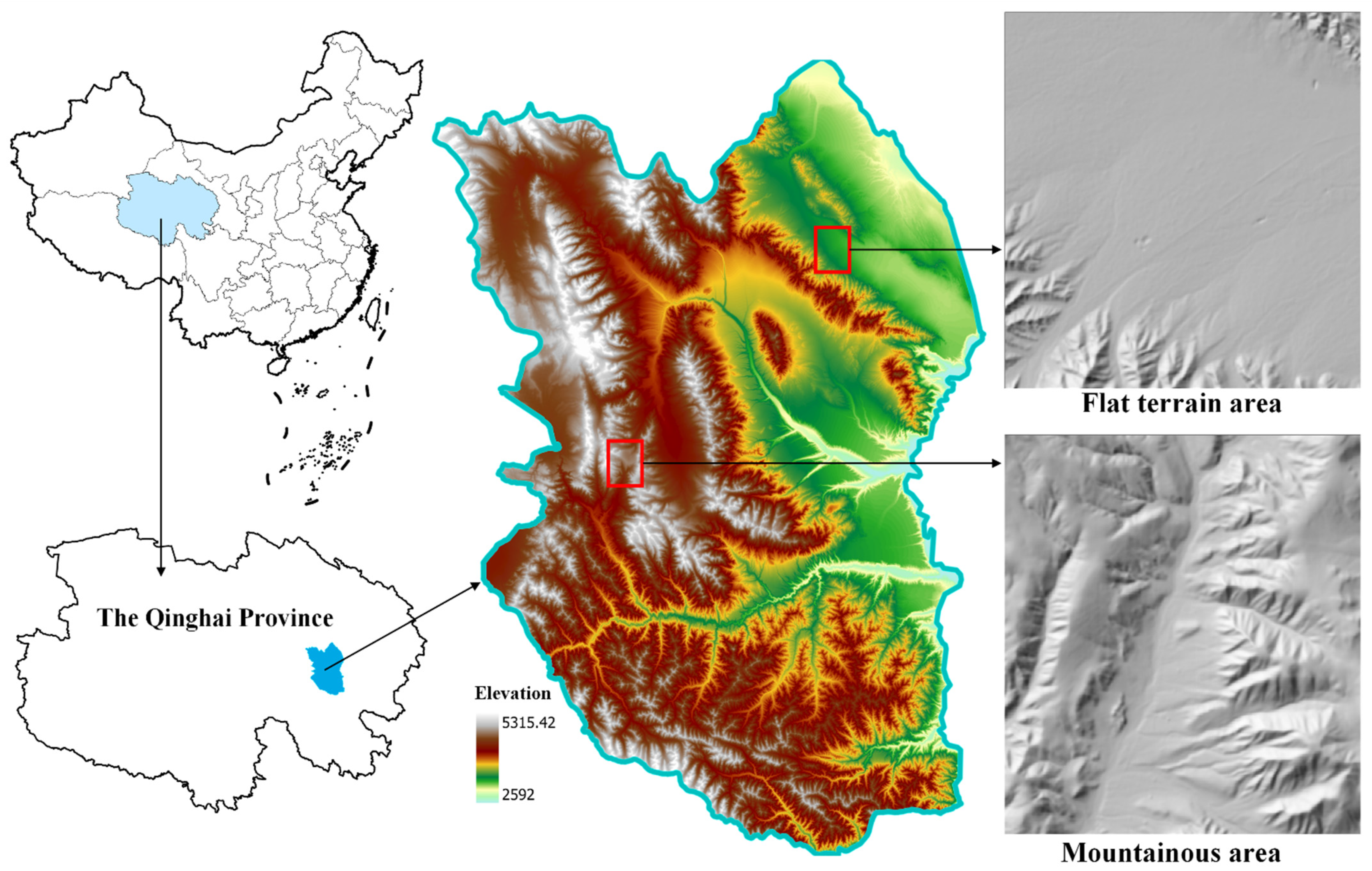
2.1. Study Area

Xinghai County is located in the eastern part of the Qinghai-Tibet Plateau, in the southwest of Qinghai Province, and is in the core area of the Sanjiangyuan National Nature Reserve. It is situated between 34°48′ N and 36°14′ N latitude and between 99°01′ E and 100°59′ E longitude. The region’s terrain is generally higher in the west and lower in the east, encompassing flat river valleys as well as mountainous areas exceeding 5000 m in elevation. Overall, the area experiences abundant sunlight and strong radiation throughout the year, with daily average temperatures ranging from −10.9 °C in January to 13 °C in July, indicating a significant annual temperature variation. Precipitation varies across the year, with higher rainfall typically occurring in June and July, while other months experience less precipitation. This area includes flat river valley landforms as well as steep mountainous regions, encompassing the land parcels and micro-slope units for research and analysis.

2.2. Elevation Data

The Copernicus program, provided by the European Space Agency (ESA), offers a Digital Surface Model (DSM) representing the Earth’s surface, including buildings, infrastructure, and vegetation [25]. Within Copernicus, three different types of DEM (Digital Elevation Model) data are available: EEA-10 data mainly cover 39 European countries with a resolution of 10 m, while GLO-30 and GLO-90 data offer global coverage with resolutions of 30 m and 90 m, respectively. This study utilizes the GLO-30 data, which have a resolution of 30 m. These data boast an absolute vertical accuracy of less than 4 m (90% linear error), a relative vertical accuracy of less than 2 m in slopes of less than or equal to 20%, and less than 4 m in slopes greater than 20% (90% linear point-to-point error within a 1° × 1° area). The absolute horizontal accuracy is less than 6 m (90% circular error) [26]. This level of uncertainty is very low as compared with the 30 m resolution of the raster dataset and the local elevation difference of terrain undulation, which is mostly above 500 m, thereby not impacting the conclusions of the research.

2.3. Principles and Software Introduction of Multi-Scale Segmentation

Multi-scale segmentation is based on the principle of minimizing regional heterogeneity. It is a bottom-up unit merging technique that minimizes internal heterogeneity within analysis units and maximizes heterogeneity between different units. The segmentation process starts by merging adjacent grid pixels with similar regional features into smaller areas. Then, these small areas are merged into larger regions based on the homogeneity principle. During the merging process, it is necessary to continually calculate whether the heterogeneity of the merged area exceeds a threshold value. If the heterogeneity is greater than the scale threshold, the two areas are not merged; if it is less than the threshold, they are combined to form a larger area. This continues until all merged areas meet the heterogeneity criteria or all areas have been iteratively processed [27]. In other words, the process of multi-scale segmentation can be understood as maximizing the non-uniformity between adjacent image units in one or multiple images under a specific segmentation scale threshold [28,29]. Furthermore, the determination of thresholds is based on the research objectives. When there are more land parcel classifications, the threshold is smaller, leading to reduced internal heterogeneity and smaller parcel areas. Conversely, when there are fewer land parcel classifications, the threshold is larger, resulting in relatively greater internal heterogeneity, larger parcel areas, and more continuity.

In this study, unsupervised clustering using k-means clustering in Rstoolbox was employed. This method divides n observations into k clusters, where each observation belongs to the cluster with the closest mean [30]. Initially, k-values are initialized by selecting initial centroids from the data points, which can be randomly selected or chosen through heuristic methods. Then, each data point is assigned to the nearest centroid based on the Euclidean distance. For each data point x_i, the nearest centroid is found, and x_i is assigned to cluster j. The process is described as follows:

$${\mathrm{S}}_{\mathrm{i}} =\{{\mathrm{x}}_{\mathrm{p}} :\left|{\mathrm{x}}_{\mathrm{p}}\right. - \left.{\mathrm{\mu }}_{\mathrm{i}}\right|\le \left|{\mathrm{x}}_{\mathrm{p}}\right. - {\left.{\mathrm{\mu }}_{\mathrm{j}}\right|}_2,{\forall }_{\mathrm{j}},1\le \mathrm{j}\le \mathrm{k}\}$$

(1)

where S_i represents the set of points allocated to the i cluster and u_i is the average value of the points in S_i. |·|₂ denotes the Euclidean norm. Next, the centroid of each cluster is updated to the average value of all points in the cluster, as expressed below:

$${\mathrm{\mu }}_{\mathrm{i} }=\frac{1}{\mid {\mathrm{S}}_{\mathrm{i}}\mid }{\displaystyle \sum _{\mathrm{x}\in {\mathrm{S}}_{\mathrm{i}}}\mathrm{x}}$$

(2)

where S_i represents the points in cluster i.

Finally, these steps are repeated until the centroids no longer change significantly or the maximum number of iterations is reached. This process aims to minimize the within-cluster sum of squares, meaning that the sum of squared distances between each data point and its centroid is minimized. However, due to varying data volumes, and based on the research objectives and computer hardware capabilities, an attempt was made to select reasonable numbers of random starts and iterations.

$$\mathrm{J}={\displaystyle \sum _{\mathrm{i}=1}^{\mathrm{k}}}{\displaystyle \sum _{\mathrm{x}\in {\mathrm{S}}_{\mathrm{i}}}(\mathrm{x}-{\mathrm{\mu }}_{\mathrm{i} }{)}^2}$$

(3)

2.4. Impact Factor

2.4.1. Basic Indicators

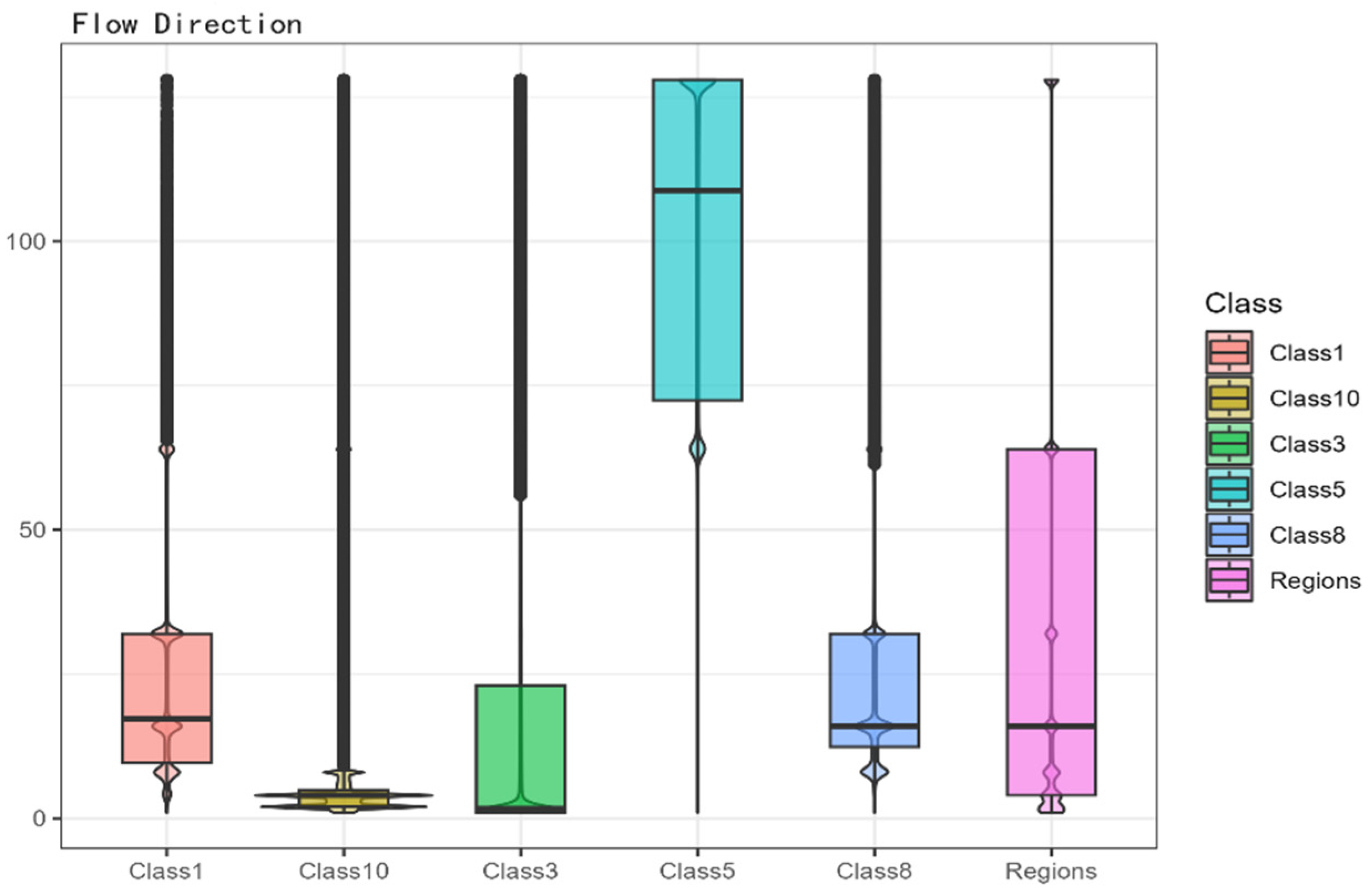
The three indicators—slope, aspect, and surface roughness—were calculated in R using the terra package. Surface curvature, flow direction, and flow accumulation were calculated in ArcGIS Pro 3.0.2.

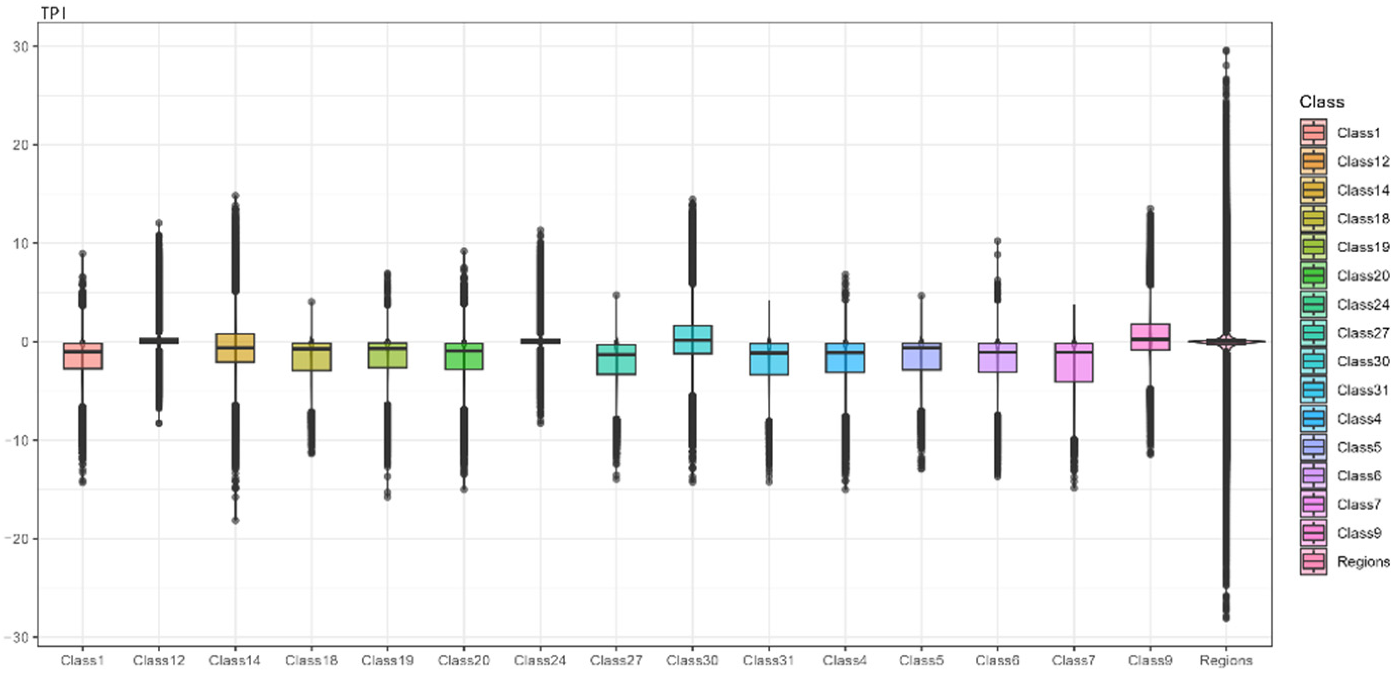
2.4.2. Topographic Position Index (TPI)

TPI, or the Topographic Position Index, compares the elevation of each grid point with the average elevation of the surrounding area. A positive TPI value indicates that the feature is higher than the average of its surrounding environment, such as a hill or ridge. A negative TPI value indicates that the feature is lower than its surroundings, like a valley or depression. A TPI value close to zero suggests that the terrain is flat or has a gentle slope.

TPI = C − M

(4)

where C denotes a particular raster image element and M denotes the average of 3 × 3 peripheral image elements around C.

2.4.3. LS

The LS factor represents the combined impact of slope length (L) and slope steepness (S) on soil erosion. Slope length is typically measured from the top of the slope to the point of deposition or to where the slope gradient decreases sufficiently for sediment to be deposited. Slope steepness refers to the angle of the slope. These factors were calculated using the following equations [31].

L = (F × c(E) + 1)^0.5

(5)

S = exp(10.6 × sin(slope) − 8.15)

(6)

LS = L × S

(7)

where L is the slope length factor, F represents flow accumulation, E is the elevation, and C refers to the pixel. S is the slope steepness coefficient, where ‘slope’ indicates the angle of the cell. The slope is typically measured in radians, and ‘exp’ refers to the exponential function.

2.4.4. Slope Aspect Variation Coefficient

In the geographical environment, ‘slope aspect variation’ typically refers to the variability or diversity of slope directions within a given area. First, we calculated the cosine and sine values of x and y coordinates.

x = cos(aspect)
y = sin(aspect)

(8)

Second, we calculated the mean values of x and y within a 3 × 3 grid surrounding each cell to determine local change patterns.

$$\begin{array}{l}\mathrm{m}\mathrm{e}\mathrm{a}\mathrm{n}\_\mathrm{x}=\frac{1}{9} {\sum }_{\mathrm{i}=1}^{3 }{\sum }_{\mathrm{j}=1}^3 {\mathrm{x}}_{\mathrm{i}\mathrm{j}} \\ \mathrm{m}\mathrm{e}\mathrm{a}\mathrm{n}\_\mathrm{y}=\frac{1}{9} {\sum }_{\mathrm{i}=1}^3 {\sum }_{\mathrm{j}=1}^3 {\mathrm{y}}_{\mathrm{i}\mathrm{j}} \end{array}$$

(9)

Third, we calculated the variance of these local changes to more accurately highlight topographical variation characteristics.

$$\mathrm{c}\mathrm{i}\mathrm{r}\mathrm{c}\mathrm{u}\mathrm{l}\mathrm{a}\mathrm{r}\_\mathrm{v}\mathrm{a}\mathrm{r}\mathrm{i}\mathrm{a}\mathrm{n}\mathrm{c}\mathrm{e}=1-\sqrt{\mathrm{m}\mathrm{e}\mathrm{a}\mathrm{n}\_{\mathrm{x}}^2+\mathrm{m}\mathrm{e}\mathrm{a}\mathrm{n}\_{\mathrm{y}}^2}$$

(10)

Fourth, we calculated the coefficient of variation for the slope aspect.

circular_sd = −2log(1 − circular_variance)

(11)

2.4.5. Surface Area Ratio (SAR)

The surface area ratio is a measure used to compare the actual surface area of the terrain with its projected area on a plane. The SAR quantifies the size of the landscape’s true surface area in comparison to the area seen on a map or a planar projection. This difference arises due to the undulations, slope, and irregularities of the terrain.

First, we calculated the gradient in the x and y directions.

$$\begin{array}{l}{\nabla }_{\mathrm{x} }=\mathrm{f}\mathrm{o}\mathrm{c}\mathrm{a}\mathrm{l}(\mathrm{e}\mathrm{l}\mathrm{e}\mathrm{v}\mathrm{a}\mathrm{t}\mathrm{i}\mathrm{o}\mathrm{n},\mathrm{w}=\frac{1}{8} \left[\begin{array}{ccc}-1& 0& 1\\ -2& 0& 2\\ -1& 0& 1\end{array}\right]\\ {\nabla }_{\mathrm{y}}=\mathrm{f}\mathrm{o}\mathrm{c}\mathrm{a}\mathrm{l}(\mathrm{e}\mathrm{l}\mathrm{e}\mathrm{v}\mathrm{a}\mathrm{t}\mathrm{i}\mathrm{o}\mathrm{n},\mathrm{w}=\frac{1}{8} \left[\begin{array}{ccc}-1& -2& -1\\ 0& 0& 0\\ 1& 2& 1\end{array}\right]\end{array}$$

(12)

Focal calculation was performed using the elevation data matrix.

$$\mathrm{S}\mathrm{A}\mathrm{R}=\sqrt{1+{\nabla }_{\mathrm{x}}^{2 }+{\nabla }_{\mathrm{y}}^2}$$

(13)

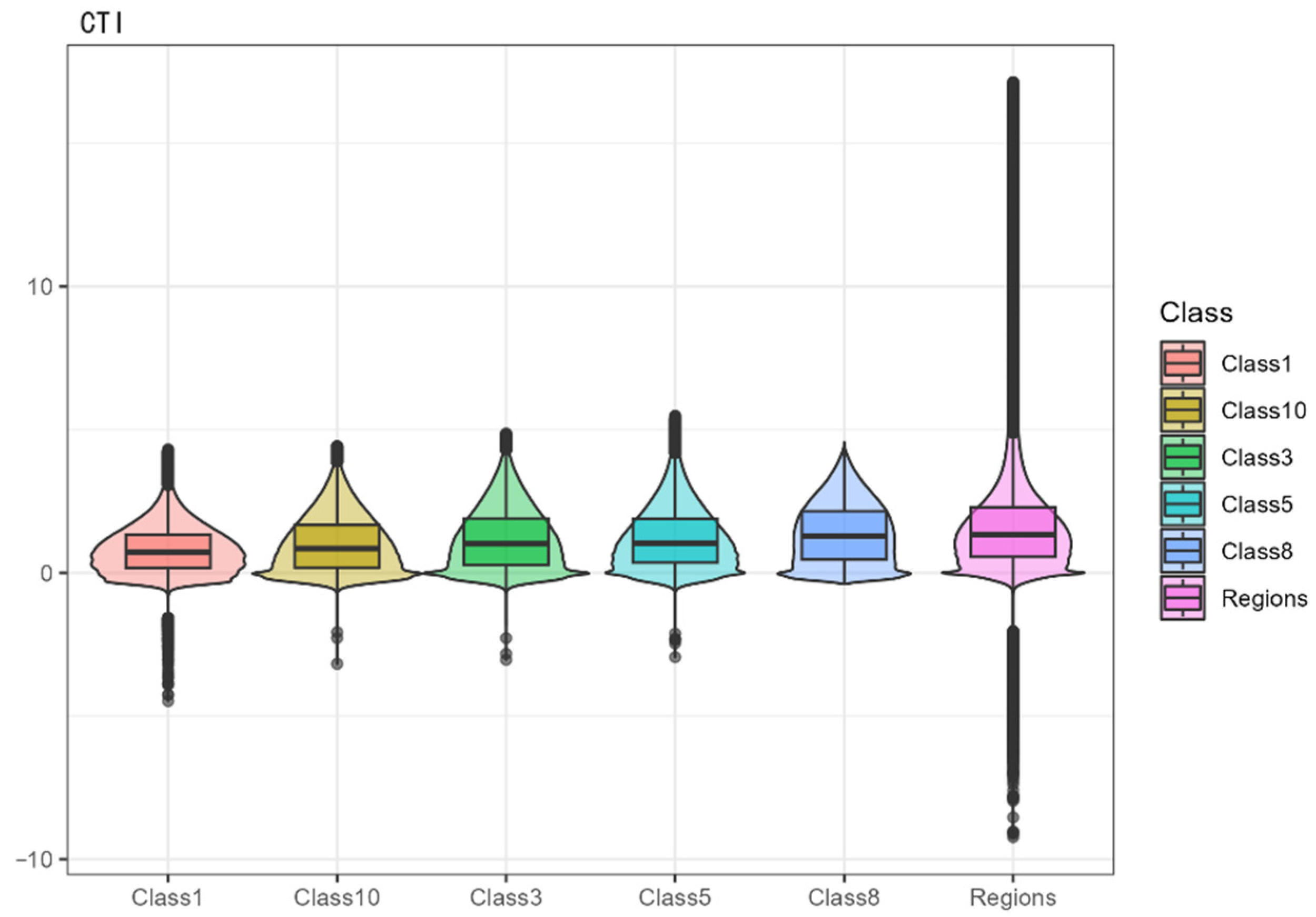
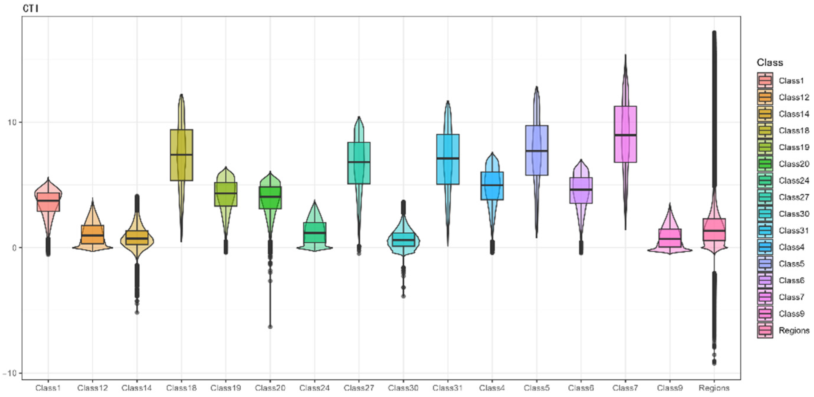
2.4.6. Compound Topographic Index (CTI)

The Compound Topographic Index (CTI), also known as the Topographic Wetness Index, is a metric used in geography and environmental science to assess the potential for water accumulation in a given landscape. The principle behind CTI is that water accumulation in the terrain is influenced by the slope and the upstream area flowing into that point. Essentially, it predicts the likelihood of water accumulation and soil moisture in different parts of the landscape.

CTI = ln(1 + F) − ln(1 + tan(S))

(14)

where F represents flow accumulation, and S represents slope.

2.5. PCA

The goal of PCA (principal component analysis) is to replace a large set of correlated variables with a smaller set of uncorrelated variables, while retaining as much information from the initial variables as possible.

For example, the first principal component is calculated as follows:

PC₁ = A₁X₁ + A₂X₂ + … + A_KX_K

(15)

This represents a weighted combination of K observed variables, offering the maximum variance explanation for the initial set of variables. The second principal component, also a linear combination of the initial variables, ranks second in terms of variance explanation and is uncorrelated with the first principal component.

Common methods for extracting the number of principal components include prior empirical and theoretical knowledge, threshold values of cumulative variance explained by the variables, and the correlation coefficient matrix among variables. In general, each principal component is associated with the eigenvalues of the correlation coefficient matrix. The first principal component is associated with the largest eigenvalue, the second principal component with the second largest eigenvalue, and so on. The Kaiser criterion suggests retaining principal components with eigenvalues greater than 1, as components with eigenvalues less than 1 explain less variance than is contained within a single variable [32].

2.6. Slope Unit Evaluation and Validation

2.6.1. Manual Extraction of Land Parcels

Based on field observations and manual drawing, we used land parcels that correspond to the meso-scale and micro-scale in Google Earth as a baseline to validate the automatic extraction results.

2.6.2. Overlap Analysis

The baseline land parcels were then intersected with multi-scale segmentation units to extract overlapping areas. However, since the units extracted through multi-scale segmentation represent continuous terrain slopes, and the manually drawn baseline units are just a single slope, the evaluation involved dividing the area of the intersected land parcel by the area of the baseline land parcel to assess the extent of overlap.

2.6.3. Statistical Indicators

Root mean square error (RMSE) is commonly used to assess the accuracy of predictive models. It measures the differences between predicted values and actual observed values. A lower RMSE value indicates a better fit of the model.

$$\mathrm{R}\mathrm{M}\mathrm{S}\mathrm{E}=\sqrt{\frac{1}{\mathrm{N}}{{\displaystyle {\sum }_{\mathrm{i}=1}^{\mathrm{N}}({\mathrm{y}}_{\mathrm{i}}-{\widehat{\mathrm{y}}}_{\mathrm{i}})}}^2}$$

(16)

where y_i represents the actual observed values, $\widehat{\mathrm{y}}$_i represents the predicted values from the model, and N is the number of observations.

Mean absolute error (MAE) serves as a performance metric for predictive models, primarily explaining and quantifying the errors in predicted values. A lower MAE value indicates higher accuracy of the model. However, compared to RMSE, MAE is less sensitive to outliers.

$$\mathrm{M}\mathrm{A}\mathrm{E}=\frac{1}{\mathrm{N}}{\displaystyle {\sum }_{\mathrm{i}=1}^{\mathrm{N}}\left|{\mathrm{y}}_{\mathrm{i}}-{\widehat{\mathrm{y}}}_{\mathrm{i}}\right|}$$

(17)

where y_i represents the actual observed values, $\widehat{\mathrm{y}}$_i represents the predicted values, and N is the total number of observations.

3. Research Design and Procedure

3.1. Research Design

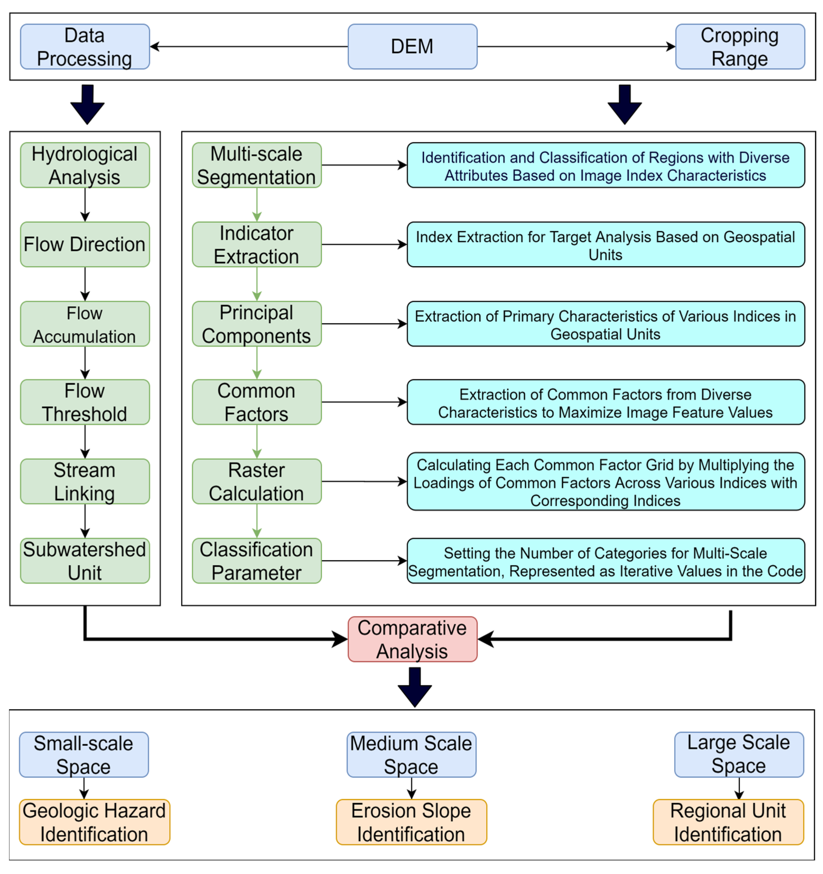
This study is divided into three parts (Figure 1). The first part employs hydrological analysis. In ArcGIS, using DEM data, watershed polygons are identified. Elevation data are processed for depression filling, calculating flow direction, and flow accumulation. Reasonable thresholds are set based on flow accumulation grids to extract rivers, followed by river linking. Watershed division is conducted based on river linking and flow direction [33], and then the necessary hydrological units are extracted.

The second part utilizes the multi-scale segmentation method. Firstly, utilizing the acquired elevation data, the necessary index factors are calculated. Secondly, principal component extraction is applied to each indicator’s loadings. Thirdly, by employing factor loadings, different principal component grids are calculated. This involves multiplying the factor loadings of various indices in the first principal component by the index factors, then summing the resultant grids to form the first principal component grid. The second principal component grid is derived in a similar manner. Fourth, land parcels are extracted using the multi-scale segmentation method. Finally, the extracted land parcels are classified, the original indicators are cropped, and mathematical statistics are performed. It is important to note that when the resolution and range of the calculated index factors differ, it is necessary to use DEM (Digital Elevation Model) elevation data as the reference dataset and resample the other index factors accordingly.

The third part compares the characteristics of slope units between the hydrological analysis method and the multi-scale segmentation method. It analyzes whether the multi-scale segmentation method can support the needs of different research objectives in terms of land parcel extraction. Initially, in large-scale spatial exploration, the identification of regional units through multiple indices is examined for its ability to meet macroscopic research needs, such as analyzing the boundaries of biological communities and climate change. However, this analysis requires additional indices and more macro-regional data. Subsequently, at a medium scale, land parcels are extracted based on multiple indices, selecting and merging terrains with the least internal heterogeneity to provide a geographical basis for hydrological process studies in land parcel units. Finally, in small-scale spaces, slope units are extracted to explore categories of slope units in areas prone to geological disasters, thereby providing a basis for the prediction and monitoring of geological hazards.

3.2. Hydrological Analysis for Extracting Land Parcels

In ArcGIS Pro, using 30 m resolution elevation data, the catchment areas were calculated with threshold values of 50, 500, 1000, and 5000 through hydrological analysis methods. Firstly, depression filling was conducted to extract flow directions, calculating the flow direction in each pixel. Secondly, flow accumulation was computed to determine the quantity of water passing through each pixel. Thirdly, various thresholds were attempted to extract river networks, calculating thresholds of 50, 500, 1000, and 5000 in relation to the study area to delineate river networks. Fourthly, the river network structure was extracted using river linking functions, forming a hierarchical structure of the river system. Finally, the catchment area function was used to extract catchment areas for different thresholds.

3.3. Extraction of Influencing Factors of Land Parcels

Land parcels exhibit different characteristics across various spatial scales and geomorphological types [25]. Based on DEM data and the requirements of the multi-scale segmentation model, relevant indicators were identified in this study, combining references [34,35]. The selected indicators included the slope, aspect, surface curvature [36], Topographic Position Index (TPI) [37,38], roughness [15,25], flow direction, flow accumulation [39], slope length ratio [36], slope aspect variability [36], surface area ratio (SAR) [40], and Compound Topographic Index (CTI) [41].

3.4. Principal Component Analysis

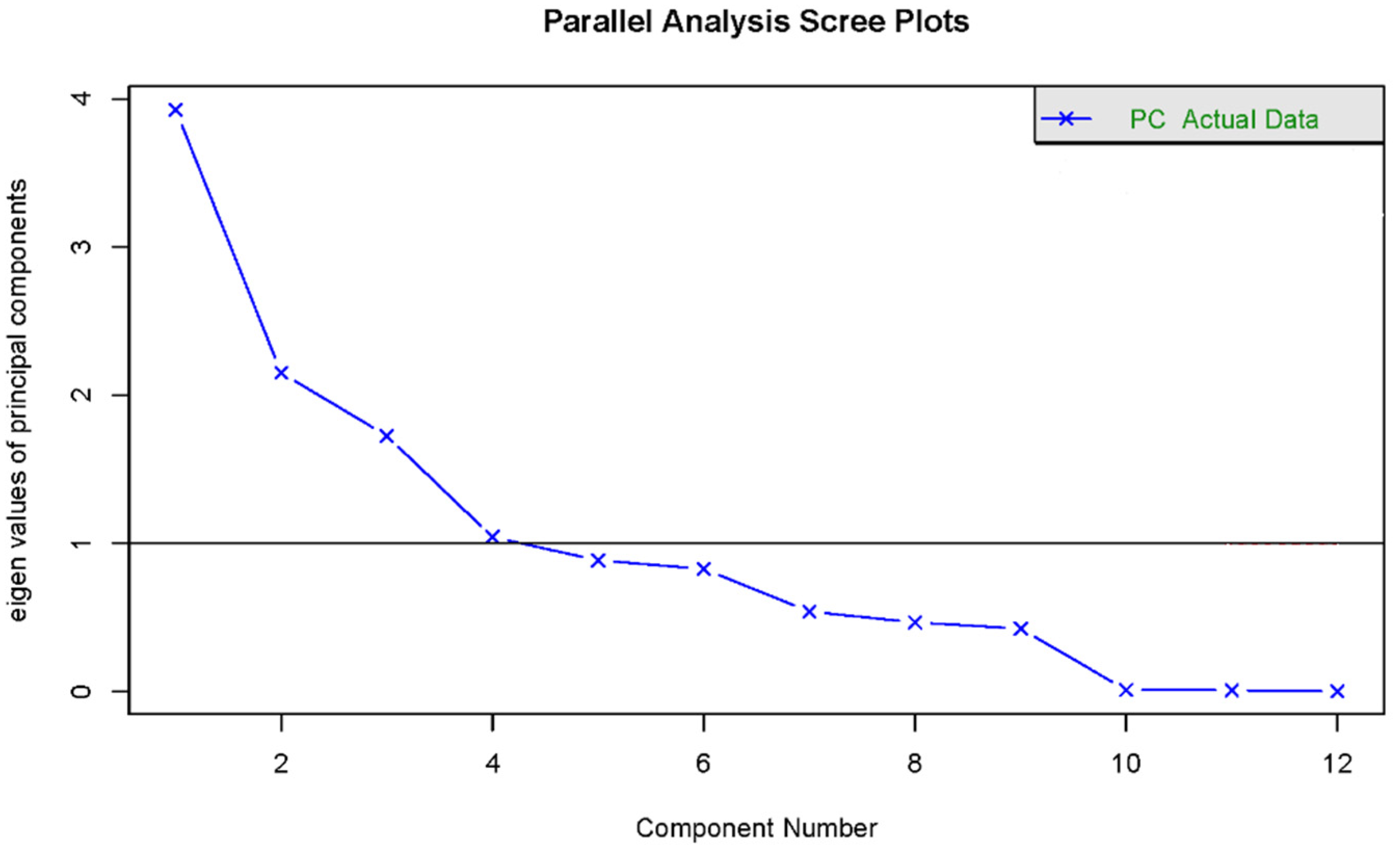
3.4.1. Determination of the Number of Principal Components

In this study, the mean eigenvalues were calculated based on 100 random data matrices. Principal components were extracted based on eigenvalues greater than 1. Scree plots of eigenvalues and principal component charts were drawn to clearly define the range of principal component variations. To facilitate the easier interpretation of the component loading matrix and to denoise the components as much as possible, varimax rotation was applied to the loading matrix, allowing each principal component to be explained by a limited set of variables. The findings indicate that four common factors can be extracted for all indicators [32] (Figure 2).

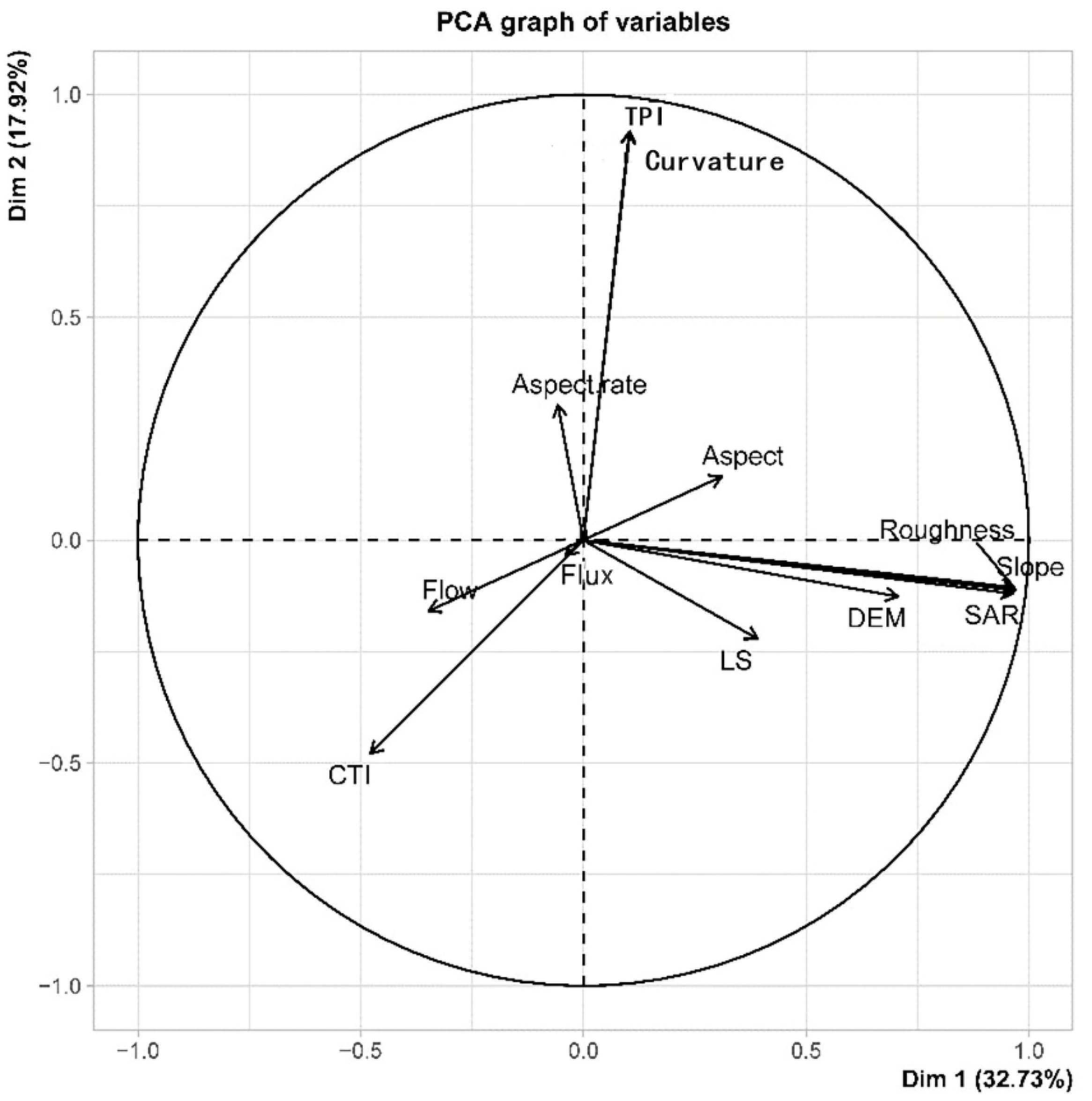
3.4.2. Identification of Principal Components

Based on the classification of principal components (Figure 3), the first principal component is primarily contributed by indicators such as elevation, roughness, surface area ratio, and slope. These four indicators mainly relate to the smoothness of the land parcels. The second principal component is mainly contributed by surface curvature and the Topographic Position Index (TPI), which primarily measure the overall undulation of the terrain. The third principal component’s main contributors are aspect, slope aspect variability, and flow direction, which are more related to the continuity of the land parcels. The fourth principal component’s main contributors are flow accumulation and the Compound Topographic Index (CTI), mainly illustrating the cumulative flow conditions of the land parcels.

3.4.3. Extraction of Common Factor Grids Based on Loadings

The loadings obtained from the principal component calculations were used as weights for the weighted operation of all indicator grids. The final grids obtained were summed up to calculate four grid images.

3.5. Construction of a Multi-Scale Segmentation Model Based on Different Scale Land Parcel Division

The multi-scale segmentation algorithm based on K-means clustering mainly extracts areas with similar land parcel properties, ensuring the minimum internal heterogeneity and maximum inter-parcel heterogeneity. Key parameters of this method include the number of random samples selected for fitting the clusters (nsamples), the number of object-oriented classification categories (nclasses), the number of random starts for the algorithm (nstarts), the maximum allowed number of iterations (niter), the standardization of image data (norm), the application of the algorithm to the corresponding number of random samples (clustermap), and the three algorithms of k-means (algorithm). The number of object-oriented classifications determines how many categories the entire area is divided into; fewer categories identify more sensitive areas within the land parcels, while more categories identify more continuous structural changes within the land parcels.

After the trials, considering the size of the study area and the representation of segmentation, we set the random sample size for multi-scale segmentation to 1000, meaning that 1000 points are randomly selected from the imagery to initiate the segmentation process. The classification threshold was set as a looping value ranging from 3 to 100 to explore the accuracy of different category classifications. The K-means algorithm’s random startup count was set to 500, implying 500 runs with different initial centroid positions. Finally, the iteration count was set to 500, based on considerations of both computational resources and optimal clustering. The parameter settings mentioned above aimed to balance the accuracy of computational results and the computational capabilities of the computer. In terms of model selection, we considered the rationality of the optimization structure based on the objective function. We compared the sum of squares for each point assigned to different clusters, examining all three algorithms, ‘Lloyd [42]’, ‘MacQueen [43]’, and ‘Hartigan-Wong [44]’, available in the Rstoolbox package. We found that the ‘Hartigan-Wong’ algorithm provided a more reasonable combination of results with land parcels in the imagery. Finally, based on the research objectives, a comparative analysis was conducted between flat and mountainous terrains (Figure 4 and

Table 1. Statistics of typical regional indicators.

	Mountainous Area				Flat Terrain Area
	Average	SD	Max	Min	Average	SD	Max	Min
Aspect	196.83	84.34	359.23	0.69	85.89	72.95	359.58	0.82
CTI	1.539	1.396	11.291	−0.580	1.865	1.593	12.307	−0.479
Curvature	0.003	0.460	2.839	−2.467	−0.002	0.277	3.358	−2.806
DEM	4367.2	213.4	4805.8	3953.8	3354.8	91.9	3779.2	3232.3
Flow	20.20	28.97	128.00	1.00	67.20	48.91	128.00	1.00
Flux	268.3	2593.5	90,670.4	0.0	750.3	7466.5	240,201.0	0.0
LS	1.063	2.103	44.788	0.000	0.170	0.577	37.899	0.000
Roughness	20.29	11.62	58.94	0.99	5.90	7.79	63.60	0.20
SAR	7.924	4.445	21.736	1.055	2.602	2.850	25.579	1.002
SAV	0.232	0.197	2.047	0.008	0.230	0.167	1.973	0.021
Slope	0.275	0.158	0.763	0.009	0.078	0.105	0.899	0.001
TPI	0.009	1.334	7.977	−6.678	−0.007	0.786	9.021	−7.815

), assessing the rationality of land parcels at the micro, meso, and macro scales.

3.6. Assessment of Land Parcels at Different Scales

The assessment and validation of land parcels were conducted from the perspectives of internal heterogeneity and the accuracy of multi-scale segmented land parcels. Due to the involvement of extensive scale information at the macroscopic level, the selected study area in this research is challenging to further analyze. Therefore, the assessment and validation were focused on land parcels at the medium and micro scales.

The assessment of land parcels at the meso and micro scales should consider three aspects—internal directional consistency, smoothness, and consistency of runoff generation. Directional consistency ensures similarity in influences like temperature and precipitation across land parcels. Smoothness determines the minimal undulation changes within slope units. Runoff consistency governs the water-collecting capacity of slope units.

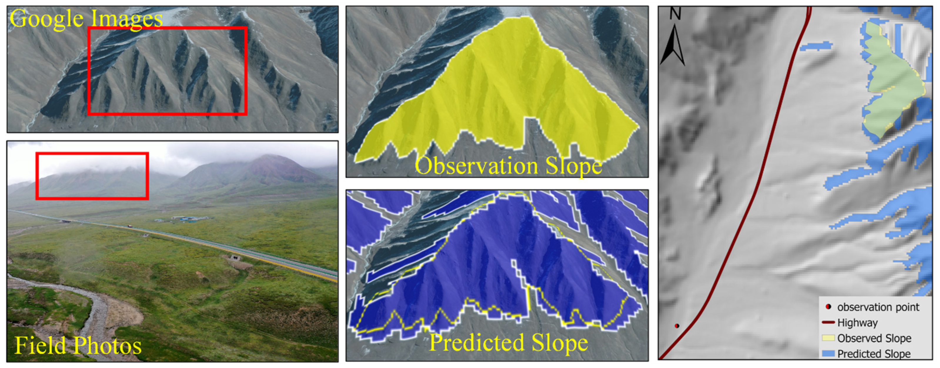
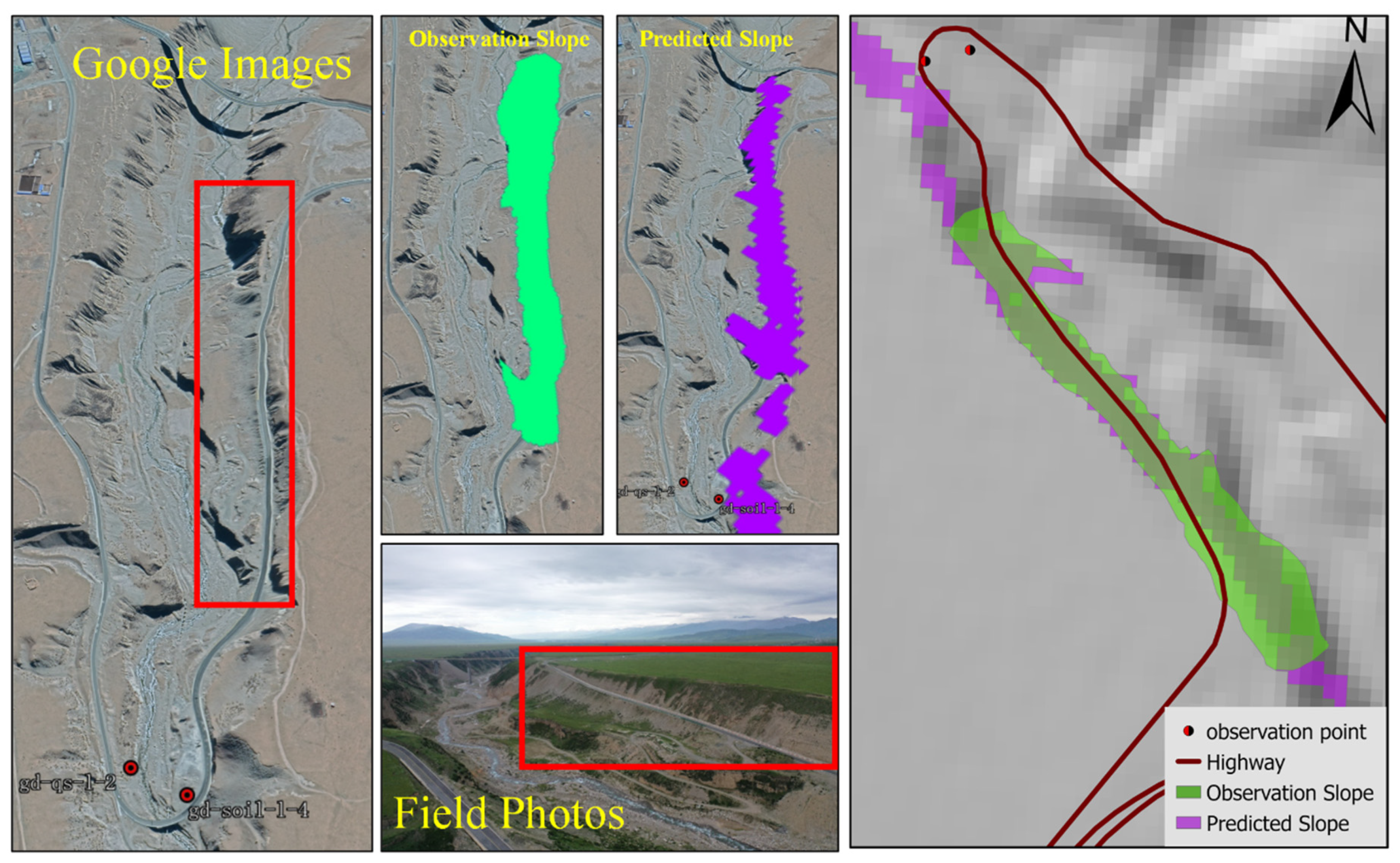
The accuracy validation of multi-scale segmented land parcels was conducted using field surveys, unmanned aerial vehicle (UAV) imagery, and high-resolution Google Earth imagery. Observation land parcels were manually delineated, with five parcels drawn for each land parcel category, resulting in a total of 100 observed land parcels. Validation methods included overlap analysis, RMSE (root mean square error), and AME (average mean error). Overlap analysis involved the intersection of observed land parcels with predicted land parcels from multi-scale segmentation. The ratio of the intersection area to the observed area was calculated to assess the effectiveness of multi-scale segmentation in representing observed land parcels. RMSE and AME were employed to evaluate the fitting performance between observed and predicted land parcels. Lower values for both metrics indicated a good fit, although RMSE is more sensitive to outliers.

4. Results

4.1. Hydrological Analysis Extracted Land Parcels

Different geomorphological units are analyzed at the micro and meso scales. Analyzing the catchment units under different thresholds reveals the following patterns (Figure 5 and Figure 6). First, the variation in catchment area extent is associated with changes in threshold values. As the threshold increases, the catchment area will encompass those of smaller thresholds, increasingly ignoring micro-geomorphological structures during the merging process. Second, rivers are the concave parts of the catchment units, with the entire catchment unit being a concave trough-like structure centered around the river. Third, river structures become sparser with increasing thresholds. Fourth, since hydrological extraction is based on elevation data, conclusions drawn from hydrological analysis in plain areas have limited practical significance for actual research. Fifth, each catchment area is an independent unit, and there is no attribute field that can categorize catchment areas with similar attributes into the same class.

4.2. Multi-Scale Segmentation Extraction of Land Parcels

Classification thresholds of 5, 19, and 31 were selected for macro, meso, and micro-scale extraction conclusions as the study subjects of land parcels. The following patterns were observed. First, regardless of mountainous or flat areas, the smaller the classification threshold, the easier it is to identify river network structures. Second, the larger the classification threshold, the more sensitive it becomes to changes in terrain slope, easily identifying land parcels at smaller spatial scales and leading to more chaotic identification results in plain areas (Figure 7). Third, at the macro scale, land parcel division focuses on river network identification, dividing the entire area into three categories. At the macroscopic scale, land parcels were grouped to achieve an average area of 3959.7 square kilometers per category. At the medium scale, land parcels were segmented to minimize heterogeneity, forming continuous slope units, with an average area of 1936.7 square kilometers per category. The largest category covered an area of 2404 square kilometers, while the smallest had an area of 1407.7 square kilometers. At the micro scale, slope units with the least heterogeneity were extracted, and slope units of similar nature were classified into one category (Figure 8), resulting in an average area of 578 square kilometers per category. The largest category covered an area of 1175.9 square kilometers, while the smallest was 71 square kilometers.

4.3. Statistical Analysis of Indicator Data for Mountainous Areas Based on Multi-Scale Segmentation

4.3.1. Meso-Scale Land Parcel Assessment

An assessment was conducted on land parcels with a classification threshold of 19, requiring the exclusion of grid cells containing river networks. The results show that five categories of land parcels were extracted. Combining the statistical conclusions of the study area, the assessment results are as follows.

Firstly, comparing the flow direction data of the entire study area (Figure 9), it was found that there is a high degree of internal consistency in the flow directions of the five types of land parcels, exhibiting good internal consistency within the land parcels. Next, the Topographic Position Index (TPI) calculated the smooth undulations of slope units (Figure 10), with convexities as positive values, concavities as negative values, and values close to zero indicating flat terrain or gentle slopes. The TPI and quartiles of the land parcels show that the extreme value ranges of the five land parcels are smaller than the entire study area, indicating internal consistency in terrain undulation within these parcels. Lastly, the Compound Topographic Index (CTI) was used to assess the consistency of runoff generation. The extreme value ranges of the five land parcels are also smaller than the entire study area, indicating that although there are differences in upstream and downstream runoff generation, there is internal consistency (Figure 11).

In summary, the five types of land parcels exhibit excellent internal consistency in flow directions. However, each type of land parcel covers a large area, leading to weaker statistical conclusions in the Topographic Position Index and Compound Topographic Index. Nevertheless, this approach provides a very good methodological system for extracting meso-scale land parcels.

4.3.2. Micro-Scale Land Parcel Assessment

An analysis was conducted on land parcels with a classification threshold of 31, similarly excluding river network structures. This resulted in the extraction of 15 types of land parcels. Combining the statistical conclusions of the entire study area, the assessment results are as follows.

Firstly, a comparison within the study area revealed that the flow direction of the 15 types of land parcels did not show significant differences (Figure 12), except for four types where the flow direction was more concentrated. Secondly, the Topographic Position Index (TPI) indicated that the extreme values of all 15 types of land parcels were smaller than the entire study area (Figure 13). For instance, in Classification 9, the mean value is 0.55 with a standard deviation of 2.28. Classification 12 exhibits a mean value of 0.23 with a standard deviation of 1.18, suggesting internal consistency in terrain undulation. Lastly, the Compound Topographic Index (CTI) revealed significant differences in upstream and downstream runoff relationships among the 15 types of land parcels. In the case of Classification 9, the mean value is 0.83 with a standard deviation of 0.89. Conversely, Classification 30 exhibits a mean value of 0.69 with a standard deviation of 0.76. These statistics indicate good internal consistency within Classification 30, which is crucial for analyzing local geological disasters such as landslides, collapses, and mudflows (Figure 14).

In summary, as the threshold value increases, the area of the extracted land parcels becomes smaller. Although internal consistency in flow direction is not evident, significant differences in terrain undulation and upstream–downstream runoff are observed, which are of great importance for the analysis of geological disasters and local areas.

4.3.3. Evaluation of Different Land Parcels at the Mesoscale

Overlap analysis indicates that the degree of overlap between land parcels observed at the mesoscale and the predicted land parcels exceeds 58%, with the lowest category at 58.66%. The reduced overlap in category 10 is due to its predicted land parcels being primarily located on large, gentle slopes with relatively flat terrain, influenced by the internal river network structure. For category 8, the lower overlap is because its predicted land parcels are situated on slopes beside river valleys, also affected by the river network structure. In summary, the algorithm’s effective recognition of river network structures leads to greater error margins between predicted and observed parcels in flatter areas. The larger mean absolute error (MAE) and root mean square error (RMSE) values for categories 10 and 8 further substantiate the significant overlap errors between the observed and predicted land parcels (Figure 15 and

Table 2. Evaluation results of mesoscale land parcels.

Name	Mean	Sd	Mae	Rmse
class 1	0.894	0.174	0.233	0.561
class 3	0.653	0.358	0.252	0.551
class 5	0.697	0.337	0.273	0.686
class 8	0.609	0.353	0.553	1.129
class 10	0.587	0.407	1.424	4.034

).

4.3.4. Evaluation of Different Land Parcels at the Microscale

The overlap analysis at the microscale showed that, apart from categories 18 and 24, where the overlap degree of observed and predicted land parcels was below 50%, and category 12, where it was 57.9%, the overlap in other categories exceeded 60%. Category 24 is located in large, gentle slopes with relatively flat terrain, while category 18 is situated on mountain slopes. Both are influenced by the river network structure, resulting in lower overlap rates between observed and predicted land parcels. The predicted land parcel of category 12 is on the opposite slope of the river valley from category 18, also affected by the extraction of the river network structure. RMSE and MAE analyses also confirm that categories 24 and 12 are more error-prone due to the influence of outliers, while the prediction errors in other models remain within the acceptable limits (Figure 16 and

Table 3. Evaluation results of microscale land parcels.

Name	Mean	Sd	Mae	Rmse
Class 1	0.769	0.271	0.074	0.132
Class 4	0.781	0.307	0.025	0.043
Class 5	0.694	0.333	0.068	0.150
Class 6	0.624	0.375	0.243	0.536
Class 7	0.797	0.155	0.020	0.055
Class 9	0.723	0.332	0.052	0.238
Class 12	0.579	0.391	0.406	0.860
Class 14	0.896	0.172	0.016	0.031
Class 18	0.495	0.369	0.323	0.581
Class 19	0.668	0.349	0.056	0.107
Class 20	0.700	0.330	0.073	0.129
Class 24	0.431	0.430	1.033	1.869
Class 27	0.715	0.325	0.218	0.489
Class 30	0.804	0.268	0.022	0.044
Class 31	0.754	0.292	0.019	0.029

).

5. Discussion

5.1. Internal Heterogeneity of Land Parcels Extracted by Hydrological Method

The goal of this study is to extract land parcels with minimal internal heterogeneity and maximal external heterogeneity. Hydrological extraction targets small watersheds, characterized by concave slope units running from the highest local points to the lowest, centered around rivers. 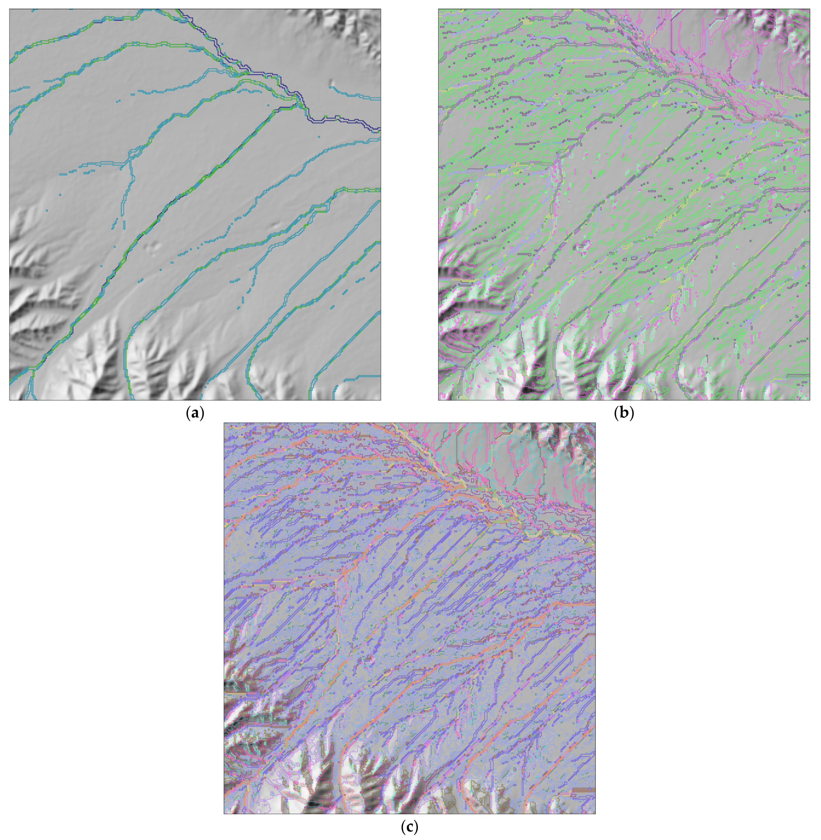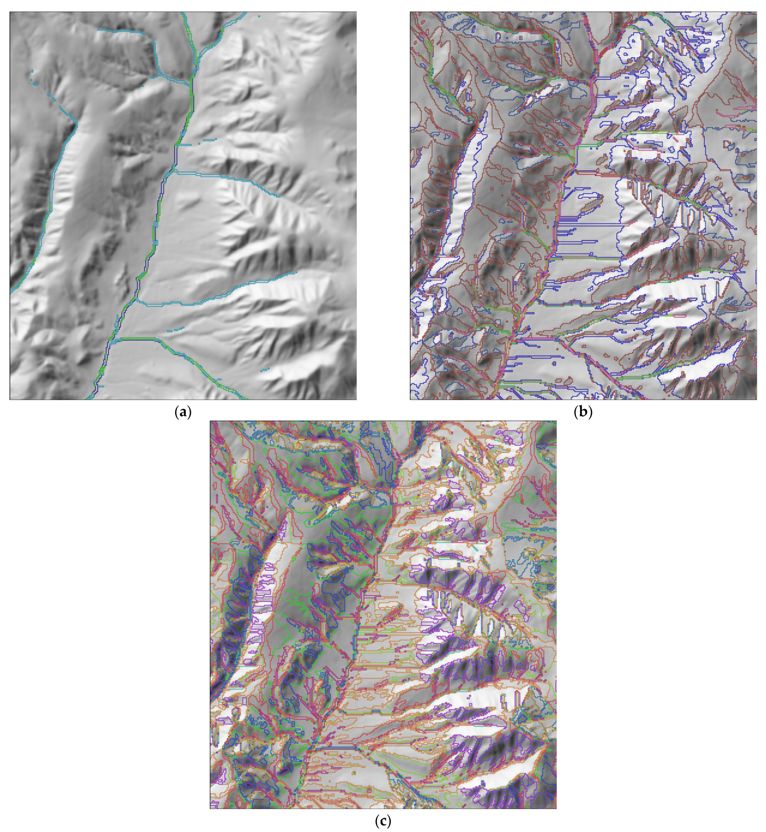However, the classification of these extracted small watersheds is weak, making it difficult to establish correlations between different watersheds, especially in large-scale areas, leading to analytical challenges [45]. Thirdly, due to differences in threshold selection, the extraction range of small watersheds changes significantly, resulting in excessive classification in flat areas without forming integral slope units. This method is relatively effective in mountainous regions, but differentiation between tributary and main river slope units is weak, and they are often classified together due to threshold influences, forming concave terrain division units.

5.2. Extraction of Land Parcels by Multi-Scale Segmentation

From a geomorphological perspective, land parcels are combinations of individual slopes, adjacent slopes, or small catchment areas [46]. In this study, micro-terrain feature differences vary at different scales, with greater internal heterogeneity at the macro scale and lesser at the micro scale. We believe that the threshold range of internal heterogeneity of land parcels is determined by different spatial research orientations. Thus, land parcels extracted at different scale thresholds can be considered continuous, uniform, and closed spatial units [24].

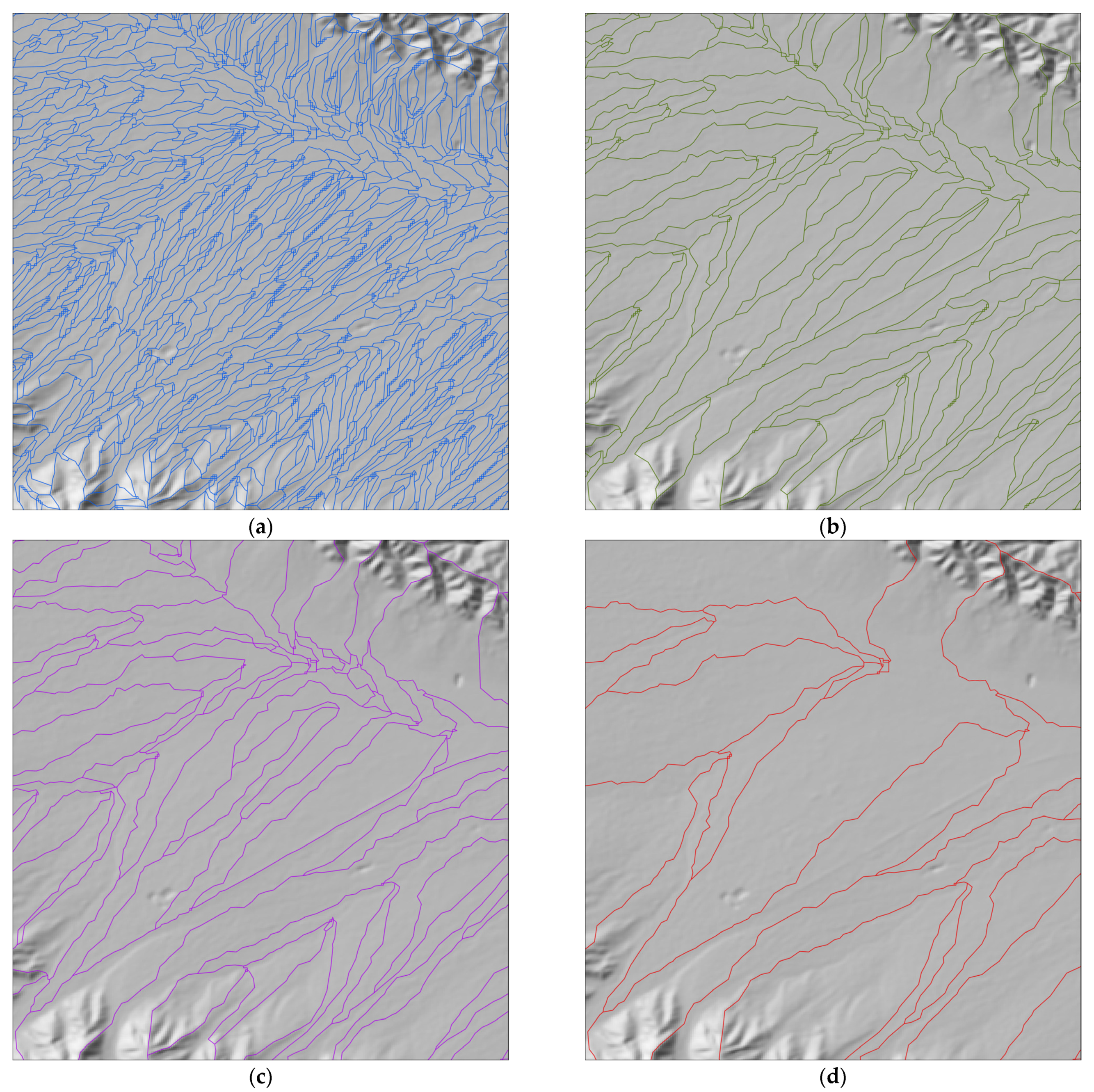
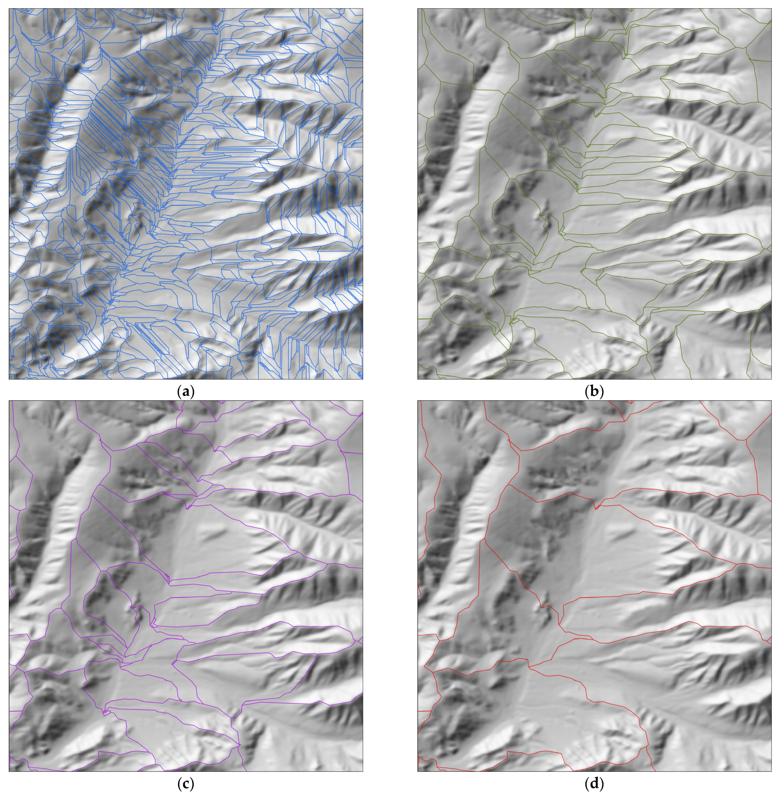
It is evident from small to large classification parameters that multi-scale segmentation is sensitive to micro-topographic undulations within the study area. With smaller classification thresholds, river networks are identified first due to significant terrain changes on both sides of the river. As parameters increase, classification spills over the riverbanks, dividing surrounding land parcels into certain categories. At a classification parameter of 5, it will identify land parcel units such as river network structures, mountainous areas, flat regions, and river valley areas; at a classification parameter of 19, large continuous slope units are recognized; and at a classification parameter of 31, finer slope units are identified, dividing the study area into irregularly shaped small patches, suitable for landslide and geological disaster zoning.

5.3. Multi-Scale Segmentation and Selection of Land Parcel Indicators

The purpose of land parcel extraction in this study is to extract slope units for analyzing soil erosion and to identify areas prone to geological disasters. Therefore, the selected indicators are all derived from calculations based on DEM (Digital Elevation Model) data. If the research objective changes, the selection of indicators can be altered accordingly. For example, some studies have used elevation, aspect, and slope data for landslide disaster identification [47,48]. Based on different research objectives, these studies have chosen various resolutions of imagery and indicators to carry out multi-scale segmentation and extract categories relevant to their research targets. In summary, multi-scale segmentation is a versatile image segmentation method. Depending on the research objective, it involves analysis combining principal component analysis or the standardization of indicator data, thus extracting the categories of objects required for the study.

5.4. Comparison of Extraction Results from Hydrological Method and Multi-Scale Segmentation

Accuracy and efficiency in land parcel extraction are important benchmarks for comparing multi-scale segmentation and hydrological analysis. The hydrological extraction method delineates concave areas centered on river channels, based on the comprehensive body of the catchment area as defined by threshold changes. However, for soil erosion and geological disaster analysis, slope units bounded by rivers are required, necessitating adjustments and corrections to the hydrological analysis, which also introduces errors. The slope units extracted by the multi-scale segmentation method merge areas with minimal internal heterogeneity and do not cross rivers, presenting complete slopes. In addition, multi-scale segmentation efficiently and accurately extracts large-scale slope units when continuous parameters are set in the code for comparative analysis.

6. Conclusions

Based on the object-oriented multi-scale segmentation method in Rstoolbox, the results demonstrate its capability in identifying land parcels based on micro-topographical variations on the surface, thus providing a complete methodological process for river network structure analysis, slope unit system classification, and micro-topographical analysis such as landslides.

(1) The land parcels extracted by the hydrological analysis method are concave structures centered around rivers, including slopes on both sides of the river. Multi-scale segmentation, centered on river valley morphological changes, can accurately identify different types of slope units on both sides of the river.

(2) This method performs well in identifying land parcels in mountainous areas. With a classification threshold of 19, the entire study area is divided into five types of land parcels, each with minimal internal heterogeneity. At a threshold of 31, the area is divided into 15 types of land parcels, with minimal internal heterogeneity in upstream and downstream runoff.

(3) The method is significantly influenced by variations in indicator datasets. It effectively identifies micro terrain variations when combined with principal component analysis. The validation results confirm that the average overlap area at the mesoscale is 69%, with the mean values of the root mean square error (RMSE) and mean absolute error (MAE) being 1.39 and 0.55, respectively. At the microscale, the average overlap area is 70%, with mean RMSE and MAE values of 0.35 and 0.18, respectively. However, after changing indicators, it was found that using only elevation, slope, and aspect data effectively identifies areas with flatter terrain. Therefore, the application of this method first depends on different research objectives, and hence different indicator structures; secondly, it depends on whether the indicator data are standardized.

Regarding considerations in future research involving object-oriented multi-scale segmentation, firstly, the accuracy of the boundary is influenced by the principal component analysis and the method of weight assignment. Secondly, when the algorithm is run in R, it consumes a substantial amount of memory resources, necessitating further enhancements in the scalability for processing large datasets. Thirdly, the capability to handle multi-modal data should be strengthened to ensure the stability and versatility of the segmentation algorithm. Finally, the application of multi-scale segmented land parcels in cold regions requires focusing on aspects such as the hydrological processes of different land parcels, changes in land use, land evaluation and management, and identification of geological disasters. Through scale variation, the universal laws governing these geographic units should be explored.