Abstract
Groundwater-dependent vegetation (GDV) is threatened globally by groundwater abstraction. Water resource managers require maps showing its distribution and habitat preferences to make informed decisions on its protection. This study, conducted in the southeast Pilbara region of Western Australia, presents a novel approach based on metrics summarising seasonal phenology (phenometrics) derived from Sentinel-2 imagery. We also determined the preferential habitat using ecological niche modelling based on land systems and topographic derivatives. The phenometrics and preferential habitat models were combined using a framework that allows for the expression of different levels of uncertainty. The large integral (LI) phenometric was capable of discriminating GDV and reduced the search space to 111 ha (<1%), requiring follow-up monitoring. Suitable habitat could be explained by a combination of land systems and negative topographic positions (e.g., valleys). This designated 13% of the study area as requiring protection against the threat of intense bushfires, invasive species, land clearing and other disturbances. High uncertainty represents locations where GDV appears to be absent but the habitat is suitable and requires further field assessment. Uncertainty was lowest at locations where the habitat is highly unsuitable (87%) and requires infrequent revisitation. Our results provide timely geospatial intelligence illustrating what needs to be monitored, protected and revisited by water resource managers.
1. Introduction
Groundwater-dependent ecosystems (GDEs) rely on groundwater to sustain their ecological function [1]. These ecosystems host a rich diversity of flora and fauna and support a range of ecosystem services such as water storage and purification [2,3]. According to Doody et al. [4], there are three main types: subterranean (aquifers and caves), aquatic (ecosystems dependent on surface expression of groundwater, such as springs) and terrestrial (ecosystems dependent on the subsurface presence of groundwater). Groundwater-dependent vegetation (GDV) can occur in both terrestrial and aquatic GDEs and comprises vegetation complexes and communities that have some level of reliance on groundwater to maintain their ability to grow and function [5,6].
Approximately one-third of the world’s vegetation is dependent on groundwater for at least some of its water requirements [7]. However, as around 40% of all global groundwater abstraction occurs in the arid regions of the world, most of the research on GDV is focused there [8]. With high daily transpiration requirements in these regions, the inability to source water from a declining water table makes them highly vulnerable to arid conditions, potentially resulting in widespread mortality [9,10,11]. Hence, GDV protection is an important consideration in water resource management [11,12], but this requires knowing its distribution and extent throughout the broader landscape [2,13].
Aerial observations have described GDV as “green islands” in contrast to the surrounding landscape [14]. This characteristic has been the basis for mapping GDV using earth observation data; GDV will possess green, moist foliage year-round if it is able to access the water table, whereas non-GDV will not [15] Barron et al. [16] exploited this characteristic in their Groundwater-dependent Ecosystem Mapping (GEM) method. The GEM method looks for minimal differences in leaf greenness and leaf moisture between wet and dry acquisitions of bi-annual Landsat imagery. They accomplish this using a combination of the normalised difference vegetation index (NDVI; Ref. [17]) and the normalised difference wetness index (NDWI; Ref. [18]), respectively.
A variation of the GEM method has been the greater use of the available temporal resolution (e.g., monthly or bi-monthly acquisitions rather than bi-annual) to explore yearly variability more finely. Several studies have summarised these acquisitions into per-pixel mean and standard deviation metrics to identify pixels with low variance, above-average greenness and, hence, typical healthy GDV characteristics (e.g., Refs. [19,20]). This advancement beyond bi-annual observations more fully utilises the seasonal phenological response of GDV and thus should smooth out any seasonal anomalies like unseasonal precipitation that may cause flushing of the understorey.
Phenometrics extend this principle further and have the potential to extract substantially more of the information available from the time series than just the mean and variance [21]. Phenometrics aim to quantify key phenological stages of plants over multiple seasons. These include statistics that relate to peak greenness, rate of greening, rate of senescence, overall productivity and the start and end of growth periods. They also have proven application in the discrimination of vegetation communities. For example, van Leeuwen et al. [22] showed that vegetation communities in wetter locations in their study area have higher productivity as well as an earlier start to the growing season than coexisting communities along a drying altitudinal gradient.
Other methods augmenting spectral data have utilised auxiliary variables at different scales. Over large areas, the Gravity Recovery and Climate Experiment (GRACE) satellite, which maps Earth’s gravity field using a K-band microwave ranging system [23], has improved our understanding of groundwater storage, although it is limited by its spatial resolution of c. 300 km [13]. At regional scales, analysis-ready layers of evapotranspiration [24], fractional cover mapping [11] and land surface temperature [25] at a coarse resolution (e.g., 500 m) have been applied. At sub-regional scales, terrain derivatives based on digital elevation models (DEMs) have been used as surrogates of landscape wetness and groundwater potential (e.g., Refs. [3,26]) and to identify suitable (and unsuitable) species habitat (e.g., Refs. [27,28,29,30]).
Contemporary models often combine spectral data with auxiliary variables to express the likelihood of a pixel being GDV [30]. This combination has been demonstrated to improve upon spectral data alone [31]. There has been a dichotomy of approaches for producing these models: (1) spatial multicriteria evaluation (SMCE) and (2) machine-learning [30]. The major differences between them are that SMCE is based on human judgement [32] whereas machine learning (e.g., random forests, neural networks) is not, and, therefore, it is less prone to procedural mistakes and perceptual bias. However, neither approach can be expected to outperform the other [30] as demonstrated by Abrams et al. [33] for groundwater mapping. Recent examples of SMCE have used the weighted linear combination method (e.g., Refs. [11,34]). A wider range of machine learning approaches have been used and include maximum likelihood classification (e.g., Ref. [3]), probabilistic frequency ratio (PFR; e.g., Ref. [33]), weights of evidence (e.g., Ref. [35]) and, in some cases, an ensemble of several (e.g., Ref. [36]).
The Dempster–Shafer theory of evidence is another branch of modelling that recognises that incomplete (fuzzy) knowledge exists in the lines of evidence (variables) being used. It has been used for groundwater potential modelling (e.g., Refs. [37,38]) but appears to be underutilised for GDV modelling per se. Like SMCE and machine learning, it can combine multiple pieces of evidence to arrive at a model representing the likelihood (belief) of GDV for each pixel. However, what distinguishes it from other techniques is its ability to also produce other useful outputs, such as the plausibility model, which represents locations where GDV could reside, even if it does not currently. These models make up the lower (belief) and upper (plausibility) bounds that a hypothesis is true and the difference between them is the degree of uncertainty, which triggers resurvey events.
The Pilbara region of Western Australia is a center of arid zone biodiversity and is globally recognised as a major producer of high-quality iron ore [39]. As iron ore mines in the area continue to mature, redirecting pit water (dewatering) to provide access to the ore beneath is becoming more common [40]. This can result in a localised lowering of the water table. If the water table is reduced beyond root limits, mortality of GDV can occur. Knowing the location of GDV will greatly assist its protection via repeat monitoring and intervention. However, none of the methods mentioned above, which are all based on the “green islands” theory, are designed to map GDV if it is already unhealthy, dead or previously existing. Therefore, we argue that GDV that can currently be detected from satellite requires consistent monitoring, particularly of its response to drawdown, and that all habitats that can plausibly host GDV, and thus can be used to infer a GDE, require protection, particularly against the threat of diminished groundwater, intense bushfires, invasive species, land clearing and other disturbances.
Our aim is to utilise a time series of remotely sensed imagery and digital elevation model derivatives to create a suite of outputs that can inform land managers where GDV currently exists and requires monitoring for change, where it could exist and requires protection, where it is unlikely to exist and can be revisited less regularly and where we need more information to improve our level of uncertainty. To achieve our aim, we seek to (a) produce a range of phenometrics and determine those suitable for GDV discrimination; (b) develop an ecological niche model showing suitable GDV habitat; (c) combine variables using Dempster–Shafer theory of evidence modelling to produce the suite of model outputs to define locations that require repeat monitoring, protection against disturbance and follow-up surveys. We expect that healthy GDV will stay greener for longer than non-GDV and thus phenometrics related to year-round greenness (e.g., productivity metrics) can be utilised to differentiate GDV. We also expect that the areas close to waterbodies and other depressions will provide the most suitable habitat. We apply our approach to a practical case study in the southeast of the arid Pilbara region of Western Australia, where damming has reduced the flow of water north of the dam wall, affecting vegetation communities, including GDV, since the early 1980s.
2. Materials and Methods
2.1. Study Area
The Pilbara bioregion [41] is approximately 180,000 km2 and is entirely contained within the arid zone [42] of Western Australia (Figure 1). It is one of only 15 national biodiversity hotspots [39]. Mean annual precipitation varies spatially from around 300–350 mm in the northeast to 250 mm in the south and west and is temporally unreliable with extended droughts not uncommon [43]. Mean annual potential evapotranspiration exceeds 3100 mm [42]. Most precipitation occurs in summer and early autumn (January to March). The convective nature of summer rain means that large amounts can be received in a single fall and is often highly localised. Winter rainfall (June–August) is usually much lower than summer and autumn and only occurs, primarily, because of elongated southern latitude fronts. Spring rain throughout the Pilbara is extremely low and usually restricted to rain in November preceding the summer wet season [44].
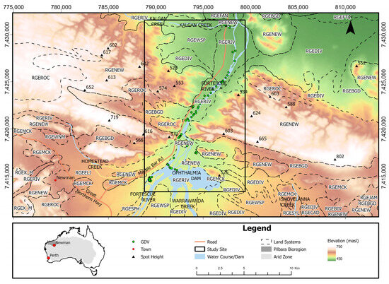
Figure 1.
Study area located on the southeastern boundary of the Pilbara bioregion in the arid zone of Australia. Elevation was sourced from the SRTM mission. Arid zone is based on Zomer et al. [42]. The Pilbara bioregion is based on the IBRA (2012) version 7 dataset [41]. Land system abbreviations are defined in Table A2.
2.2. GDV Species
The flora in the Pilbara bioregion is diverse, with 1137 vascular species (1094 were native) recorded during surveys undertaken in the late 1990s [44]. Phreatophytes are used to infer the presence of a groundwater-dependent ecosystem [1]. These species draw water from the phreatic zone and can usually be found along streams where there is a steady flow of surface or groundwater or consistent pooling where the water table is near the surface. They contrast in appearance from coexisting vadophytes (Figure 2A), which have no dependence on groundwater. Eucalyptus victrix L.A.S. Johnson and K.D. Hill (Coolibah; Figure 2B), E. camaldulensis subsp. refulgens Brooker and M.W. McDonald (River Red Gum; Figure 2C) and Melaleuca argentea W. Fitzg (Silver Cadjeput; Figure 2D) are the three most common “GDV species” in the Pilbara bioregion.
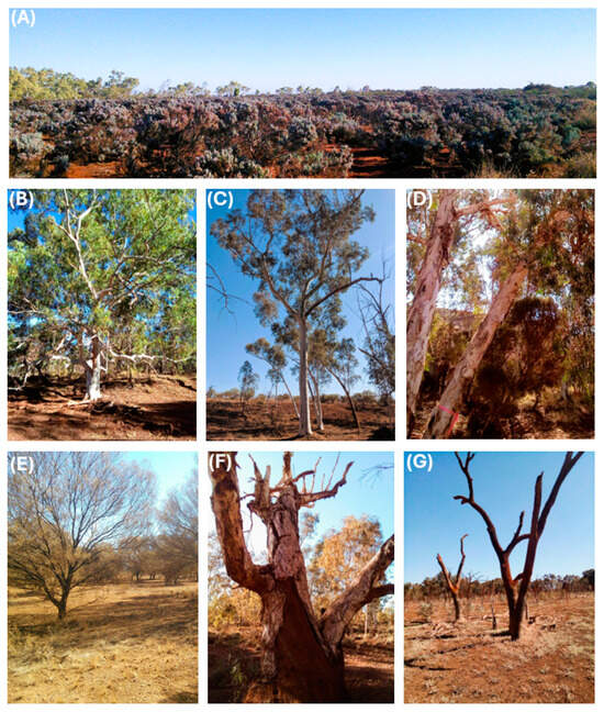
Figure 2.
(A) Groundwater-dependent vegetation species appear as “green islands” in the background in contrast to the saltbush (Atriplex sp.) in the foreground, which has no groundwater dependence. (B) Example of a healthy Eucalyptus victrix with a health rating of 5 (see text). (C) Example of a E. calmuldulensis with a health rating of 4 due to some leaf loss on lower limbs. (D) Example of a healthy Melaleuca argentea. (E) Acacia species, which are common vadophytes in the uplands. (F) Dead mature M. argentea tree. (G) Dead E. calmuldulensis.
2.3. Study Site and Field Data
The study site, located in the southeast corner of the Pilbara bioregion, covers an area of c. 20,000 ha in the vicinity of Ophthalmia Dam (Figure 1). The dam was constructed in 1981 by Mt. Newman Mining Company Pty Ltd. approximately 19 km east of the town of Newman (Figure 1) for town and mining water supply. Post-construction, there has been negligible downstream contribution and a restriction of flood events that is partially responsible for vegetation condition decline north of the dam wall [45,46].
Field observations focused on GDV species around the dam and up to 16 km north of it. These samples were acquired opportunistically using GPS-enabled tablets running ArcGIS Collector [47] in late August 2019. GDV species were recorded along with a health score from 1–5, where 1 signified a dead plant, 3 signified branches without leaves and 5 was a perfectly healthy specimen. For the purposes of this study, we grouped GDV species together and removed any with health ratings less than 4, leaving a sample size of 119 observations (Figure 1). This was randomly split into two 50% partitions used for training (N = 60) and model validation (N = 59). We did not record non-GDV plant species.
M. argentea is considered an obligate phreatophyte, requiring permanent surface and near-surface water for survival and has the most dependence on groundwater of the three observed [48]. Mortality is rapid if groundwater becomes unavailable (Figure 2F). While it is common near creeks throughout the Pilbara, it was not observed in our survey in the vicinity of the dam. E. camuldulensis and E. victrix were observed. Both are facultative phreatophytes because they can grow in areas where groundwater is not available and satisfy water requirements from unsaturated zones but will use groundwater if it is available [49,50]. If established over shallow groundwater, they are likely to develop groundwater dependence and have higher vigour and better stand development due to increased water uptake [51]. However, such dependence makes them vulnerable if groundwater becomes unavailable, depending on the rate of groundwater drawdown. There appears to be a correlation between size and groundwater dependence, with the health of large E. camuldulensis trees (>10 m tall) found to decline in response to groundwater levels lowering, while smaller examples are less impacted [52].
2.4. Datasets
We acquired one cloud-free Sentinel 2A/B image from approximately the first week of each month of 2019 from the Sentinel Australasia Regional Access (SARA) catalogue. This was achievable for all months except April, which was interpolated by averaging the March and May acquisitions (Table A1). We used the hydrologically enforced 30 m resolution digital elevation model (DEM) acquired by the Shuttle Radar Topography Mission (SRTM—https://pid.geoscience.gov.au/dataset/ga/72759 (accessed on 22 November 2024)) for all terrain derivatives. Land systems, which tie together geographical, geological and ecological data, were sourced from van Vreeswyk et al. [44]. The land systems displayed in Figure 1 are defined in Table A2.
2.5. Phenometric Modelling
2.5.1. Moisture-Adjusted Vegetation Index
All Sentinel images were transformed into a time series of moisture-adjusted vegetation index (MAVI) layers as described by Zhu et al. [53]:
where NIR is near-infrared reflectance (c. midpoint = 0.865 µm), RED is reflectance in the red wavelengths (c. midpoint = 0.665 µm) and SWIR is reflectance in the shortwave infrared (c. midpoint = 1.61 µm). These bands correspond to bands 8, 4 and 11 of Sentinel-2, respectively.
2.5.2. Description of Phenometrics
The MAVI time series was smoothed by fitting a Savitzky–Golay function using TIMESAT version 3.3 [54]. Ten phenometrics were extracted based on the smoothed function as defined in Table 1. Figure 3 provides an illustration to accompany the definitions.

Table 1.
Summary of phenometrics derived from the time series of Sentinel-2.
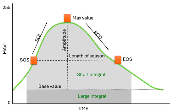
Figure 3.
Illustration of the phenometrics extracted from the Sentinel time series. See Table 1 for definitions.
2.5.3. Choosing Between Phenometrics
A correlation coefficient was calculated between all pairs of phenometrics to identify variable redundancy. All phenometrics with a correlation ≥ 0.90 were removed. The remaining phenometrics were then run through MaxENT software v. 3.3.3 [55] singularly using the training dataset (N = 60), and an area under the curve (AUC) was computed from the corresponding receiver-operating characteristic (ROC) curve [56] based on the testing dataset. A ROC curve is a graph of the false-positive rate (x-axis) against the true-positive rate (y-axis). ROC curves that are close to the top left-hand corner illustrate a good-fitting model and will have a high corresponding AUC [57]. The AUC is a summary performance measurement that is calculated using the trapezoidal rule of the area under the ROC [58]. In our implementation, the AUC measures how much separability there is between GDV and background samples (other land covers). An AUC of 1 indicates perfect separation, whereas 0.5 denotes an unusable model because true positives and false positives are not distinguishable [59]. We calculated the AUC for all variables together and proceeded to reduce the full model by removing the poorest single model (lowest AUC) at each iteration. This allowed for the most parsimonious set of phenometrics to be retained. We plot the response curves of retained variables to describe the relationship between each phenometric and GDV.
2.6. Ecological Niche Modelling
The SRTM DEM was resampled to 10 m resolution to match the Sentinel imagery using cubic convolution in ArcGIS PRO v. 3.1 [60]. As topography is a first-order control on the spatial variation of hydrological conditions, and groundwater flow often follows surface topography [61], we derived three raster surfaces from the DEM, which have been shown to be related to water runoff and pooling [27]: convexity, topographic position index (TPI) and the saga wetness index (SWI). All metrics were computed in SAGA software v. 7.8.2 [62]. Convexity (CON) controls the direction of flow and transport of materials and deposition of soil. Hills have high convexity and thus high runoff, whereas incised streams are concave in shape and thus receive and move water [63]. The TPI compares the elevation of each cell in a DEM to the mean elevation of a specified neighbourhood around that cell and was calculated using a 100 × 100 m neighbourhood window. Positive TPI values represent locations that are higher than the average of their neighbourhood window (e.g., ridges) and whose negative values are lower (e.g., valleys), with flat areas close to 0 [64]. The SWI was used to quantify the topographic control of hydrological processes [65]. Higher values receive more water. Finally, we also included the layer of land systems in our model.
Variables were assessed for multicollinearity, where any with a correlation ≥ 0.90 were removed and the remaining set was run through MaxENT. Backward selection based on the AUC was performed to retain the most parsimonious set of variables representing suitable GDV habitats.
2.7. Uncertainty Modelling
Uncertainty modelling identifies that there may be incomplete knowledge in the body of evidence (e.g., it may be anecdotal, indirect or come from different sources at different scales and with some inherent inaccuracy). Uncertainty modelling frequently uses the evidential belief function theory developed by Dempster [66,67] and added to by Shafer [68], coined the Dempster–Shafer theory by Barnett [69]. This theory allows for the mapping of the spatial distribution of uncertainty, where a pixel might contain GDV but the combination of evidence is insufficient to be certain [70].
Unlike traditional Bayesian probability theory, under the Dempster–Shafer belief theory, there is no requirement for probability not committed to a particular hypothesis to be committed to its negation [70,71]. This is arranged via a frame of discernment (aka as a universe of discourse) where all possible hypotheses and combinations of hypotheses are disclosed. In our approach, we have two singleton hypotheses; a pixel is either GDV or it is not GDV. Hence, our frame of discernment, Θ = {GDV, NOT GDV}, will accept evidence for all possible combinations, {GDV}, {NOT GDV} and {GDV, NOT GDV}. The latter, the non-singleton set, represents our ignorance or an inability to commit to either singleton hypothesis.
Layers are assigned to the hypotheses, and each pixel is given a basic probability assignment (BPA). A BPA represents the mass of support (m) of one of the hypotheses, and not its proper subsets. For example, if the BPA representing the support that a piece of evidence provides of an individual pixel supporting the hypothesis {GDV} is 0.6, then m({GDV}) = 0.6 and the remainder is committed to the non-singleton hypothesis representing ignorance, m({GDV, NOT GDV}) = 0.4. It could be GDV but we do not know, and more evidence is required. In our implementation, the phenometrics model was used to support the hypothesis of {GDV} and the ENM was inverted and used to support the hypothesis {NOT GDV}. We reasoned that suitable habitat does not ensure the presence of GDV species, but unsuitable habitat is good evidence in support of a location not hosting GDV. As the two models were scaled from 0 to 1, each pixel already had an appropriate BPA assigned.
The mathematics of Dempster–Shafer Belief Modelling (DSBM) allows for four mappable degrees of belief: belief, plausibility, disbelief, and belief interval [72]. Belief is the total support for a hypothesis drawn from the BPAs for all subsets of that hypothesis [73]:
where BEL(X) is the total support for a hypothesis, drawn from the BPAs for all subsets of that hypothesis. Thus, BEL({GDV}) is the sum of the BPAs, m(Y), for the hypothesis {GDV} and represents the probability that a pixel is GDV.
BEL(X) = ∑ m(Y) when Y⊆X
Plausibility is the degree to which a hypothesis cannot be disbelieved; conditions (e.g., habitat) appear to be right but hard evidence is lacking. It is calculated thusly [73]:
where = not X. Hence, PL({GDV}) is equal to 1 − BEL{NOT GDV} or 1 − DIS(X).
Disbelief is the degree of support for all hypotheses that do not intersect with that hypothesis and is, therefore, clearly associated with plausibility [73]:
where = not X. Hence, DIS({GDV}) is equal to BEL{NOT GDV}.
The range between plausibility (the upper bound of belief) and belief (the lower bound of belief) is the belief interval and represents the doubt or uncertainty in the hypothesis [73]:
BELINT(X) = PL(X) − BEL(X)
Image Thresholding
ROC analysis can also be used for determining the threshold values for dichotomising continuous layers into binary layers. Several threshold determination methods exist, and the choice between them is based on map use (e.g., Ref. [74]). We chose to balance the importance of the false positive and true-positive rates, which corresponds to the value closest to the top northwest corner of the ROC plot [75,76]. This was performed using Youden’s J Statistic and identifying the corresponding cutoff [77]:
J = MAX(True-Positive Rate + False-Positive Rate − 1)
We used this approach to threshold the belief map to delineate likely GDV populations that require follow-up monitoring of anomalous spectral responses that may indicate stress from groundwater drawdown. We also used this technique to delineate a plausible habitat that requires protection.
3. Results
3.1. Phenometric Modelling
Correlation analysis revealed considerable multicollinearity between the ten phenometrics. Hence, only four were retained for further analysis as they had pairwise correlations below 0.9 (Figure 4A). These were length of season (LOS), rate of increase (ROI), rate of decrease (ROD) and the large integral (LI). The AUC statistics for each phenometric are also presented in Figure 4A and illustrate the discrimination potential of several. The full model combining all four uncorrelated phenometrics produced an AUC of 0.99, which did not decline during backwards stepwise elimination. The only variable retained was the LI. The response curve for the LI shows that the probability of GDV increases sigmoidally up to a value of 600 (MAVI is stored as an 8-byte integer), with all higher values very likely GDV (Figure 5).
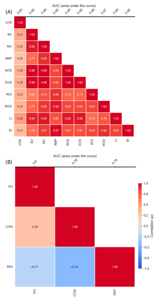
Figure 4.
Correlation matrix with individual area under the curve (AUC) statistics for (A) phenometric variables defined in Table 1 and (B) DEM derivatives (CON = convexity, TPI = topographic position index, SWI = SAGA wetness index) used in ecological niche modelling.
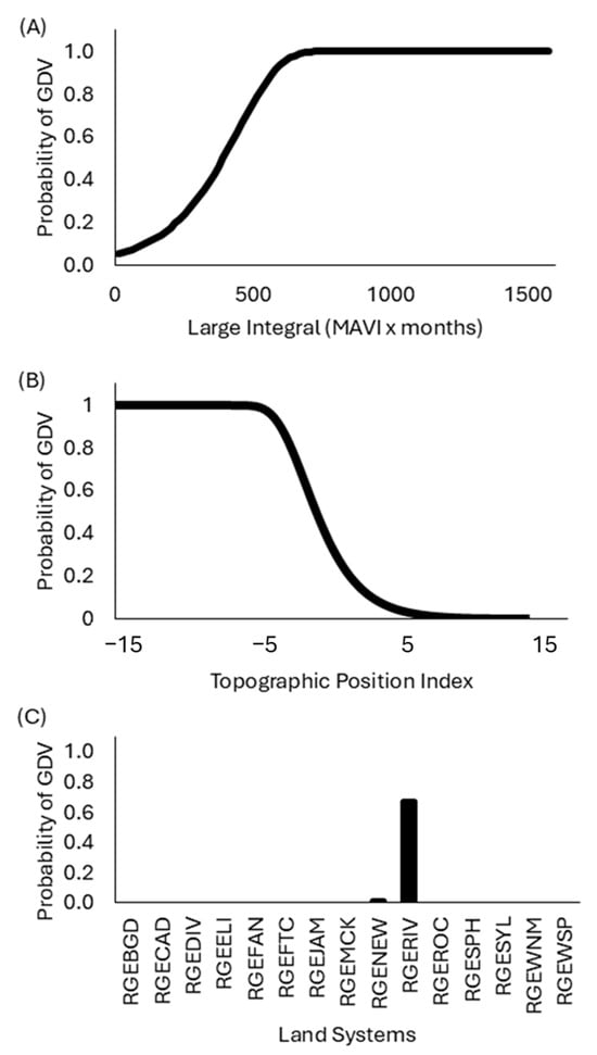
Figure 5.
Response curves for each of the retained variables of (A) the large integral, where MAVI is expressed as an 8-byte integer. The probability of GDV increases with higher values of the large integral. (B) The topographic position index showing the probability of GDV increases when it is negative. (C) Land systems showing the majority of GDV samples are found within the “River” land system (RGERIV) with a minor association with the “Newman” land system (RGENEW). See Table A2 for other definitions.
3.2. Ecological Niche Modelling
None of the potential variables for ecological niche modelling (ENM) were found to be highly correlated (r > 0.9), and so all were initially retained (Figure 4B). As the land systems were categorical, they were not tested against the other variables. AUC statistics computed for each variable on their own revealed that the land systems were the most accurate layer (AUC = 0.85). The full model produced an AUC = 0.91. Stepwise removal showed no reduction in AUC when CON and the SWI were removed but did show a slight reduction (AUC = 0.89) when the TPI was, and so it was retained. The final ENM had an AUC = 0.92 (an improvement on the full model) and identified the key determinant of GDV habitat to be the river land system, which delineates seasonally active flood plains and major river channels (Figure 5B) and where the TPI is negative (Figure 5C).
3.3. Uncertainty Modelling
The model based on the phenometrics was used in support of the hypothesis {GDV} and is shown in Figure 6A. The high-likelihood areas are those that are greener for longer periods of the year than other vegetation and, therefore, have the characteristics expected to be GDV (Figure 6A). The inverted ecological niche model is used in support of the hypothesis of {NOT GDV} and shows the upland areas as habitats that are highly likely to be suitable for non-GDV (Figure 6B).
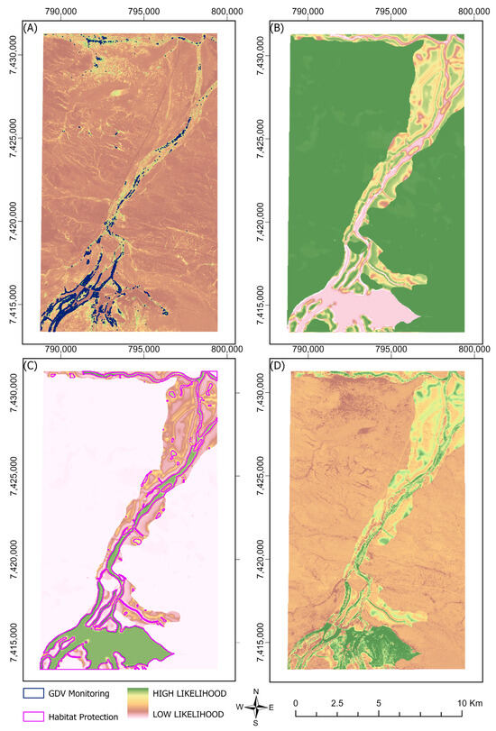
Figure 6.
Groundwater-dependent vegetation model results. (A) The BELIEF map, which represents locations in support of GDV presence. Thresholding GDV is delineated in blue. (B) The DISBELIEF map, which represents locations in support of GDV absence. (C) The PLAUSIBILITY map, which illustrates potential GDV habitat that needs protection. Suggested habitat for protection is delineated in purple. (D) The BELIEF INTERVAL map, where high belief intervals present an opportunity for further sampling to reduce uncertainty.
The plausibility map is a complement of the map of disbelief and shows locations where the habitat is suitable for GDV (Figure 6C) but does not infer GDV to be present (unlike the belief map). It shows the upper boundary of our commitment to the hypothesis {GDV} and hence has a wider range of suitable locations relative to the map of belief. Highly plausible areas closely follow the stream network. The belief interval represents the degree of uncertainty in a pixel, satisfying either the belief or the disbelief hypotheses (Figure 6D). The areas with the highest belief interval have habitats that appear to be suitable for GDV, but there is currently no concrete evidence of it being there. These areas are predominantly on the banks of watercourses in proximity to existing and predicted GDV and represent locations where follow-up field visits would have the most value in reducing uncertainty. Areas shaded in white to light brown satisfy either the belief or disbelief hypotheses and no further information is required.
Image Thresholding
ROC curves corresponding to the belief and plausibility models are shown in Figure 7. The optimal threshold for the belief model was found to be a model value > 0.75. This threshold allows for a 2% false-positive rate and a 98% true-positive rate (see blue lines, Figure 7A). This means that any thresholded pixel chosen at random will be GDV 98% of the time. Rarely (2% of the time), it will be a different vegetation type with a similar spectral response to GDV. The patches of GDV are shown in blue in Figure 6A and indicate plants that need to be monitored for changes in vigour. The optimal threshold for the plausibility model was 0.58 and returned a false-positive rate of 19% and a true-positive rate of 96% (see purple lines, Figure 7B). The preferred GDV habitat is shown delineated in purple in Figure 6C and indicates habitats that need to be protected from disturbances.
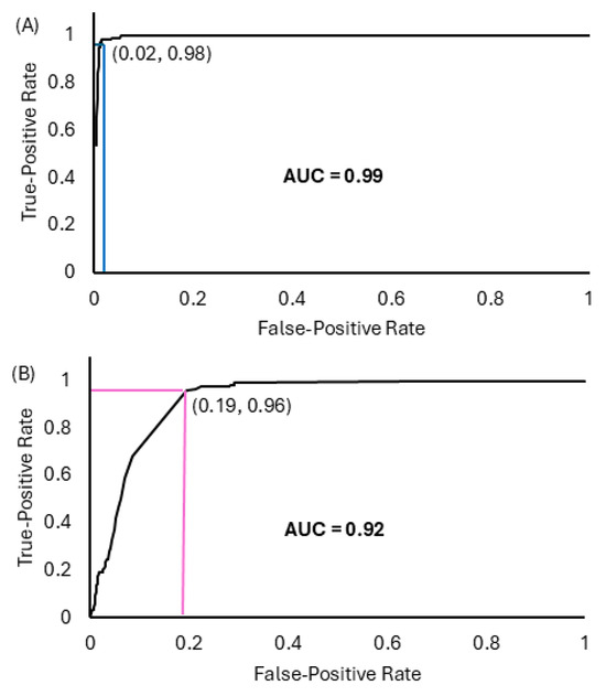
Figure 7.
Receiver operating characteristic (ROC) curves illustrating the true and false-positive rates overall threshold values. Chosen thresholds are shown in blue and purple and correspond to the models of (A) belief and (B) plausibility, respectively, and relate to the delineations in the same colour in Figure 6.
4. Discussion
The importance of groundwater for maintaining the health of GDV and associated ecosystems has become more widely recognised in recent years. Nonetheless, GDV remains under threat globally due to unsustainable levels of abstraction, causing groundwater depletion [78]. The ongoing monitoring of existing GDV communities and the protection of highly suitable habitats is needed urgently but this will be underpinned by accurately knowing their current locations and spatially defining their environmental niche, respectively. Our uncertainty modelling framework demonstrates that this can be achieved by leveraging a combination of phenometic and ecological niche modelling.
4.1. Phenometric Modelling
The use of a time series of remotely sensed imagery, rather than annual or biannual acquisitions (e.g., Ref. [15]), has previously been recommended for mapping GDV [79] and has led to an uptake of various time series-based approaches (e.g., Refs. [3,25,80]). Nonetheless, phenometric modelling for GDV mapping remains rare, although research is emerging on its use for monitoring the impact of different mining-induced disturbances on the surrounding vegetation [81,82]. In our implementation, we identified the large integral to be the most useful phenometric for characterising GDV, and it was able to differentiate GDV from non-GDV almost perfectly (AUC = 0.99). This was achieved as it relates to the evergreen appearance of GDV that contrasts with seasonally green vegetation, like grasses, or less vigorous vadophytes, which are not dependent on groundwater. It also demonstrates that the 10 m resolution of Sentinel is a suitable resolution to minimise spectral mixing and thus confusion of these land covers, which was not achieved using the 30 × 30 m resolution Landsat imagery in the study by Barron et al. [16]. As this evergreen characteristic is generally ubiquitous amongst all GDV, we expect that the large integral will be portable to most systems. One notable exception is blue oak trees (Quercus douglasii) in California [83], which are GDV but also deciduous. Even so, other phenometrics are likely to provide discrimination and the procedure for choosing between them will not change.
In addition to the large integral, we identified other candidate phenometrics with discrimination potential based on individual AUC values (Figure 4A), including the start of season (SOS) and end of season (EOS). Conceptually, SOS and EOS are akin to selecting imagery at the start of the dry season and at the end of the wet season. This is the theory underpinning the GEM model [16] and may partially explain why they were able to obtain high accuracy (e.g., 91%) in some areas with only two images. However, this needs further testing and expansion.
4.2. Ecological Niche Modelling
The TPI, CON and SWI were all found to be strong variables with AUC values between 0.78 and 0.80, which is consistent with the findings of recent similar studies (e.g., Refs. [3,34]). However, we were able to omit CON and SWI without loss of model accuracy. We also found that most GDV was confined to one land system (“River”), which delineates major river channels and serves as a surrogate for proximity to water as used by Duran-Llacer et al. [34]. Our response curves identified that GDV preferred negative TPI values, which indicates suitable habitats where the elevation is lower than its immediate surrounds (e.g., incised streams).
4.3. Uncertainty Modelling and Image Thresholding
ROC thresholding delineated 111 ha as GDV requiring repeat monitoring (Figure 6A). This equates to narrowing the search space for existing GDV to less than 1% of the study area and to be suitable for drone missions for more detailed exploration. However, unlike Bayesian modelling, this does not allow one to assume the other 99% is unsuitable. For example, plausibility modelling identified 2653 ha, or around 13%, of suitable habitat for GDV, even if it is not currently growing there. The complement of this is the disbelief model, which suggests that 87% of the study area is not suitable for GDV and can be monitored infrequently.
The plausible areas were identified throughout the riparian zone and require protection to deliver ecosystem resilience against the threat of intense bushfires, invasive species, land clearing and other disturbances to counterbalance anthropogenic impacts, including mining and pastoralism. Due to their rich biodiversity, riparian zones are also known to be effective corridors for a variety of fauna, including feral cats, which threaten important native bird species that utilise the existing GDV as safe havens for nesting and migration, in addition to ground-dwelling mammals (e.g., quolls and bilbies) and reptiles [39,84].
Weeds are another major threat to riparian zones, as they compete with native vegetation [39,85], including GDV, and modify habitat for native fauna, often amplifying the issue of feral fauna (cats and pigs). The most significant weeds are ecosystem-transforming [39] and include woody perennials such as highly invasive mesquite (Prosopis spp.) populations, parkinsonia (Parkinsonia aculeata), calotropis (Caloptropis procera) and date palms (Phoenix dactylifera). Protection must include the immediate removal of these species from GDV habitat.
The belief interval (Figure 6D) highlights locations where GDV has not been detected spectrally but that are highly plausible habitats. This layer is key to reducing uncertainty in future iterations. This can be achieved through additional surveys or new layers of spatial information. For example, Brim Box et al. [80] used a depth of groundwater layer to rule out the potential for GDV. In their study, if the groundwater was beyond 10 m, then it was deemed unsuitable habitat for Melaleuca species. Similarly, E. victrix stands where the depth of groundwater exceeded 10 m were unlikely to be utilising the groundwater and so were ruled out. This would require a high-resolution layer of groundwater interpolated from a network of piezometers. While bore fields do exist throughout the Pilbara region, they are too scattered to be relied on as a persistent data source for modelling. Generally, for much of the Pilbara region, the presence of GDV species has been used to infer groundwater depth, rather than the other way around.
4.4. Recommendations
For simplicity, we have grouped GDV species together. One source of heterogeneity is thus the proportion of each individual species at different locations. Hence, the next level of mapping should consider species discrimination or at least obligate versus facultative phreatophytes. Obligate species have no drought resistance and die rapidly without access to groundwater [86]. This is important because obligate species (e.g., M. Argentea) require different groundwater resource management and likely even stricter monitoring than the facultative species. In addition, we recommend the mapping of non-GDV species to rule them out as false positives.
There is a paucity of freely available digital elevation models for the study area. This required resampling 30 m resolution SRTM data to 10 m. We suspect some smoothing may have occurred in the resampling because there are very fine detailed locations in the belief map, based on 10 m Sentinel imagery, where GDV is likely to occur, which escapes the plausibility map, which was based on resampled SRTM (c.f. Figure 6A,C). Lidar and multispectral sensors attached to a drone would make for an impressive dataset for this purpose, as adopted by Tweed et al. [19] and Perez Hoyos et al. [13]. We recommend that it be captured monthly to enable the creation of a similar set of phenometrics.
5. Conclusions
Modelling under uncertainty provides useful geospatial intelligence in the pursuit of sustainable groundwater management. GDV, at our study site, can be modelled and mapped based on the characteristic that it will, when healthy, remain greener for longer than non-GDV. The large integral of a time series of moisture-adjusted vegetation indices captures this characteristic well and can considerably reduce the search space for monitoring (e.g., <1% of the study area).
Suitable habitat could be explained by a combination of land systems and topographic position, where negative topographic positions (e.g., valleys) were favoured. These areas could plausibly host GDV and require protection against the threat of groundwater abstraction, intense bushfires, invasive species, land clearing and other disturbances.
The greatest uncertainty was found in locations where GDV appears to be absent but the habitat is suitable. These are the locations requiring more investigation to refine the model. This may include follow-up surveys or the introduction of new information (e.g., depth of groundwater).
Author Contributions
Conceptualisation, T.P.R., L.T. and G.W.W.-J.; methodology, T.P.R., L.T. and G.W.W.-J.; validation, T.P.R. and L.T.; formal analysis, T.P.R. and L.T.; investigation, T.P.R. and L.T.; data curation, T.P.R. and L.T.; writing—original draft preparation, T.P.R.; writing—review and editing, T.P.R., L.T. and G.W.W.-J.; visualisation, T.P.R. and L.T.; project administration, T.P.R.; funding acquisition, T.P.R. All authors have read and agreed to the published version of the manuscript.
Funding
This research was funded by Spatial Information Systems Research Ltd., Project No 5E01—Measuring and Monitoring Vegetation Health Impact through Earth Observation.
Data Availability Statement
The original contributions presented in this study are included in the article; further inquiries can be directed to the corresponding author.
Acknowledgments
The authors would like to thank Bart Huntley and Jennifer Carter for their feedback on earlier versions of this manuscript and all members of the ENVestigator team for helpful discussion throughout the project. Thank you to Mandy Robinson for assistance with proofreading.
Conflicts of Interest
The authors declare no conflicts of interest. The funders had no role in the design of the study; in the collection, analyses, or interpretation of data; in the writing of the manuscript; or in the decision to publish the results.
Appendix A
Table A1.
Sentinel imagery acquired for this study.
Table A1.
Sentinel imagery acquired for this study.
| Collection | Acquisition Date | Platform | Instrument | Product | Orbit Number | Processing Level |
|---|---|---|---|---|---|---|
| S2 | 9 January 2019 | S2B | MSI | S2MSIL2A | 17 | L2A |
| S2 | 3 February 2019 | S2A | MSI | S2MSIL2A | 17 | L2A |
| S2 | 5 March 2019 | S2A | MSI | S2MSIL2A | 17 | L2A |
| - | Interpolated | - | - | - | - | - |
| S2 | 4 May 2019 | S2A | MSI | S2MSIL2A | 17 | L2A |
| S2 | 3 June 2019 | S2A | MSI | S2MSIL2A | 17 | L2A |
| S2 | 3 July 2019 | S2A | MSI | S2MSIL2A | 17 | L2A |
| S2 | 7 August 2019 | S2B | MSI | S2MSIL2A | 17 | L2A |
| S2 | 5 September 2019 | S2B | MSI | S2MSIL2A | 17 | L2A |
| S2 | 5 October 2019 | S2B | MSI | S2MSIL2A | 17 | L2A |
| S2 | 5 November2019 | S2B | MSI | S2MSIL2A | 17 | L2A |
| S2 | 5 December 2019 | S2B | MSI | S2MSIL2A | 17 | L2A |
Table A2.
Land systems found within the study area.
Table A2.
Land systems found within the study area.
| Code | Name | Description |
|---|---|---|
| RGEBGD | Boolgeeda | Stony lower slopes and plains below hill systems supporting hard and soft spinifex grasslands or mulga shrublands. |
| RGECAD | Cadgie | Hardpan plains with thin sand cover and sandy banks supporting mulga shrublands with soft and hard spinifex. |
| RGEDIV | Divide | Gently undulating sandplains with minor dunes, supporting hard spinifex hummock grasslands with numerous shrubs. |
| RGEELI | Elimunna | Stony plains on basalt supporting sparse acacia and cassia shrublands and patchy tussock grasslands. |
| RGEFAN | Fan | Washplains and Gilgai plains supporting groved mulga tall shrublands and minor tussock grasslands. |
| RGEFTC | Fortescue | Alluvial plains and flood plains supporting patchy grassy eucalypt and acacia woodlands and shrublands and tussock grasslands. |
| RGEJAM | Jamindie | Stony hardpan plains and rises supporting groved mulga shrublands, occasionally with spinifex understorey. |
| RGEMCK | McKay | Hills, ridges, plateaux remnants and breakaways of meta sedimentary and sedimentary rocks supporting hard spinifex grasslands with acacias and occasional eucalypts. |
| RGENEW | Newman | Rugged jaspilite plateaux, ridges and mountains supporting hard spinifex grasslands. |
| RGERIV | River | Narrow, seasonally active flood plains and major river channels supporting moderately close, tall shrublands or woodlands of acacias and fringing communities of eucalypts, sometimes with tussock grasses or spinifex. |
| RGEROC | Rocklea | Basalt hills, plateaux, lower slopes and minor stony plains supporting hard spinifex and occasionally soft spinifex grasslands with scattered shrubs. |
| RGESPH | Spearhole | Gently undulating gravelly hardpan plains and dissected slopes supporting groved mulga shrublands and hard spinifex. |
| RGESYL | Sylvania | Gritty surfaced plains and low rises on granite supporting acacia–eremophila–cassia shrublands. |
| RGEWNM | Wannamunna | Hardpan plains and internal drainage tracts supporting mulga shrublands and woodlands and occasionally eucalypt woodlands. |
| RGEWSP | Washplain | Hardpan plains supporting groved mulga shrublands. |
References
- Eamus, D.; Froend, R. Groundwater-dependent ecosystems: The where, what and why of GDEs. Aust. J. Bot. 2006, 54, 91–96. [Google Scholar] [CrossRef]
- Brown, J.; Bach, L.; Aldous, A.; Wyers, A.; DeGagné, J. Groundwater-dependent ecosystems in Oregon: An assessment of their distribution and associated threats. Front. Ecol. Environ. 2010, 9, 97–102. [Google Scholar] [CrossRef]
- El-Hokayem, L.; De Vita, P.; Conrad, C. Local identification of groundwater dependent vegetation using high-resolution sentinel-2 data—A Mediterranean case study. Ecol. Indic. 2023, 146, 109784. [Google Scholar] [CrossRef]
- Doody, T.; Hancock, P.; Pritchard, J. Assessing groundwater-dependent ecosystems: IESC information guidelines explanatory note. In Report Prepared for the Independent Expert Scientific Committee on Coal Seam Gas and Large Coal Mining Development Through the Department of the Environment and Energy, Commonwealth of Australia; IESC: Canberra, Australia, 2019. [Google Scholar]
- Eamus, D.; Froend, R.H.; Loomes, R.C.; Hose, G.; Murray, B. A functional methodology for determining the groundwater regime needed to maintain the health of groundwater-dependent vegetation. Aust. J. Bot. 2006, 54, 97–114. [Google Scholar] [CrossRef]
- Zhu, J.; Yu, J.; Wang, P.; Zhang, Y.; Yu, Q. Interpreting the groundwater attributes influencing the distribution patterns of groundwater-dependent vegetation in northwestern China. Ecohydrology 2011, 5, 628–636. [Google Scholar] [CrossRef]
- Barbeta, A.; Peñuelas, J. Relative contribution of groundwater to plant transpiration estimated with stable isotopes. Sci. Rep. 2017, 7, 10580. [Google Scholar] [CrossRef]
- Wada, Y.; van Beek, L.P.; van Kempen, C.M.; Reckman, J.W.; Vasak, S.; Bierkens, M.F. Global depletion of groundwater resources. Geophys. Res. Lett. 2010, 37, L20402. [Google Scholar] [CrossRef]
- Antunes, C.; Díaz Barradas, M.C.; Zunzunegui, M.; Vieira, S.; Pereira, Â.; Anjos, A.; Correia, O.; Pereira, M.; Máguas, C. Contrasting plant water-use responses to groundwater depth in coastal dune ecosystems. Funct. Ecol. 2018, 32, 1931–1943. [Google Scholar] [CrossRef]
- Jin, X.; Liu, J.; Wang, S.; Xia, W. Vegetation Dynamics and their response to groundwater and climate variables in Qaidam Basin, China. Int. J. Remote Sens. 2016, 37, 710–728. [Google Scholar] [CrossRef]
- Fildes, S.G.; Doody, T.M.; Bruce, D.; Clark, I.F.; Batelaan, O. Mapping groundwater dependent ecosystem potential in a semi-arid environment using a remote sensing-based multiple-lines-of-evidence approach. Int. J. Digit. Earth 2023, 16, 375–406. [Google Scholar] [CrossRef]
- Rohde, M.M.; Froend, R.; Howard, J. A global synthesis of managing groundwater dependent ecosystems under sustainable groundwater policy. Groundwater 2017, 55, 293–301. [Google Scholar] [CrossRef] [PubMed]
- Pérez Hoyos, I.; Krakauer, N.; Khanbilvardi, R.; Armstrong, R. A review of advances in the identification and characterization of groundwater dependent ecosystems using geospatial technologies. Geosciences 2016, 6, 17. [Google Scholar] [CrossRef]
- Everitt, J.H.; Deloach, C.J. Remote Sensing of Chinese Tamarisk (Tamarix chinensis) and associated vegetation. Weed Sci. 1990, 38, 273–278. [Google Scholar] [CrossRef]
- Liu, C.; Liu, H.; Yu, Y.; Zhao, W.; Zhang, Z.; Guo, L.; Yetemen, O. Mapping groundwater-dependent ecosystems in arid Central Asia: Implications for controlling regional land degradation. Sci. Total Environ. 2021, 797, 149027. [Google Scholar] [CrossRef] [PubMed]
- Barron, O.V.; Emelyanova, I.; Van Niel, T.G.; Pollock, D.; Hodgson, G. Mapping groundwater-dependent ecosystems using remote sensing measures of vegetation and moisture dynamics. Hydrol. Process. 2012, 28, 372–385. [Google Scholar] [CrossRef]
- Kriegler, F.J.; Malila, W.A.; Nalepka, R.F.; Richardson, W. Preprocessing transformations and their effect on multispectral recognition. Remote Sens. Environ. 1969, VI, 97–132. [Google Scholar]
- Gao, B. NDWI—A normalized difference water index for remote sensing of vegetation liquid water from space. Remote Sens. Environ. 1996, 58, 257–266. [Google Scholar] [CrossRef]
- Tweed, S.O.; Leblanc, M.; Webb, J.A.; Lubczynski, M.W. Remote Sensing and GIS for mapping groundwater recharge and discharge areas in salinity prone catchments, southeastern Australia. Hydrogeol. J. 2006, 15, 75–96. [Google Scholar] [CrossRef]
- Mackey, B.; Berry, S.; Hugh, S.; Ferrier, S.; Harwood, T.D.; Williams, K.J. Ecosystem greenspots: Identifying potential drought, fire, and climate-change micro-refuges. Ecol. Appl. 2012, 22, 1852–1864. [Google Scholar] [CrossRef]
- Jönsson, P.; Eklundh, L. Seasonality extraction by function fitting to time-series of satellite sensor data. IEEE Trans. Geosci. Remote Sens. 2002, 40, 1824–1832. [Google Scholar] [CrossRef]
- Van Leeuwen, W.J.D.; Davison, J.E.; Casady, G.M.; Marsh, S.E. Phenological characterization of Desert Sky Island vegetation communities with remotely sensed and climate time series data. Remote Sens. 2010, 2, 388–415. [Google Scholar] [CrossRef]
- Luthcke, S.B.; Rowlands, D.D.; Sabaka, T.J.; Loomis, B.D.; Horwath, M.; Arendt, A.A. Chapter 10: Gravimetry measurements from space. In Remote Sensing of the Cryosphere; Tedesco, M., Ed.; Wiley Blackwell: Oxford, UK, 2015; pp. 231–247. ISBN 9781118368855. [Google Scholar]
- Qiu, Y.; Wang, D.; Yu, X.; Jia, G.; Li, H. Effects of groundwater table decline on vegetation in groundwater-dependent ecosystems. Forests 2023, 14, 2326. [Google Scholar] [CrossRef]
- Gow, L.J.; Barrett, D.J.; Renzullo, L.J.; Phinn, S.R.; O’Grady, A.P. Characterising groundwater use by vegetation using a surface energy balance model and satellite observations of land surface temperature. Environ. Model. Softw. 2016, 80, 66–82. [Google Scholar] [CrossRef]
- Sarkar, S.K.; Rudra, R.R.; Talukdar, S.; Das, P.C.; Nur, S.; Alam, E.; Islam, K.; Islam, A.R. Future groundwater potential mapping using machine learning algorithms and climate change scenarios in Bangladesh. Sci. Rep. 2024, 14, 10328. [Google Scholar] [CrossRef] [PubMed]
- Robinson, T.; Di Virgilio, G.; Temple-Smith, D.; Hesford, J.; Wardell-Johnson, G. Characterisation of range restriction amongst the rare flora of Banded Ironstone Formation ranges in semiarid south-western Australia. Aust. J. Bot. 2019, 67, 234–247. [Google Scholar] [CrossRef]
- Keppel, G.; Robinson, T.P.; Wardell-Johnson, G.W.; Yates, C.J.; Van Niel, K.P.; Byrne, M.; Schut, A.G.T. A low-altitude mountain range as an important refugium for two narrow endemics in the southwest Australian Floristic Region Biodiversity Hotspot. Ann. Bot. 2016, 119, 289–300. [Google Scholar] [CrossRef] [PubMed][Green Version]
- Yates, C.J.; Robinson, T.P.; Wardell-Johnson, G.W.; Keppel, G.; Hopper, S.D.; Schut, A.G.T.; Byrne, M. High species diversity and turnover in granite inselberg floras highlight the need for a conservation strategy protecting many outcrops. Ecol. Evol. 2019, 9, 7660–7675. [Google Scholar] [CrossRef] [PubMed]
- Díaz-Alcaide, S.; Martínez-Santos, P. Review: Advances in groundwater potential mapping. Hydrogeol. J. 2019, 27, 2307–2324. [Google Scholar] [CrossRef]
- Al Saud, M. Mapping potential areas for groundwater storage in Wadi Aurnah Basin, western Arabian Peninsula, using remote sensing and geographic information system techniques. Hydrogeol. J. 2010, 18, 1481–1495. [Google Scholar] [CrossRef]
- Agarwal, E.; Agarwal, R.; Garg, R.D.; Garg, P.K. Delineation of Groundwater Potential Zone: An AHP/ANP approach. J. Earth Syst. Sci. 2013, 122, 887–898. [Google Scholar] [CrossRef]
- Abrams, W.; Ghoneim, E.; Shew, R.; LaMaskin, T.; Al-Bloushi, K.; Hussein, S.; AbuBakr, M.; Al-Mulla, E.; Al-Awar, M.; El-Baz, F. Delineation of groundwater potential (GWP) in the Northern United Arab Emirates and Oman using geospatial technologies in conjunction with simple additive weight (SAW), Analytical Hierarchy Process (AHP), and probabilistic frequency ratio (PFR) techniques. J. Arid. Environ. 2018, 157, 77–96. [Google Scholar] [CrossRef]
- Duran-Llacer, I.; Arumí, J.L.; Arriagada, L.; Aguayo, M.; Rojas, O.; González-Rodríguez, L.; Martínez-Retureta, R.; Oyarzún, R.; Singh, S.K. A new method to map groundwater-dependent ecosystem zones in semi-arid environments: A case study in Chile. Sci. Total Environ. 2022, 816, 151528. [Google Scholar] [CrossRef] [PubMed]
- Ahmed, M.; Niyazi, B. Groundwater Potential Mapping Using Remote Sensing Techniques and Weights of Evidence GIS Model: A Case Study from Wadi Yalamlam Basin, Makkah Province, Western Saudi Arabia. Environ. Earth Sci. 2015, 74, 5129–5142. [Google Scholar] [CrossRef]
- Jari, A.; Bachaoui, E.M.; Hajaj, S.; Khaddari, A.; Khandouch, Y.; El Harti, A.; Jellouli, A.; Namous, M. Investigating machine learning and ensemble learning models in groundwater potential mapping in arid region: Case study from Tan-tan water-scarce region, Morocco. Front. Water 2023, 5, 1305998. [Google Scholar] [CrossRef]
- Nampak, H.; Pradhan, B.; Manap, M.A. Application of GIS based data driven evidential belief function model to predict groundwater potential zonation. J. Hydrol. 2014, 513, 283–300. [Google Scholar] [CrossRef]
- Ghorbani Nejad, S.; Falah, F.; Daneshfar, M.; Haghizadeh, A.; Rahmati, O. Delineation of groundwater potential zones using remote sensing and GIS-based data-driven models. Geocarto Int. 2016, 32, 167–187. [Google Scholar] [CrossRef]
- Booth, C.; Adams, V.; Kruse, B.; Douglass, L. The Enduring Pilbara: A conservation vision for a land rich in nature, culture and resources. In The Enduring Pilbara; Centre for Conservation Geography and University of Tasmania: Hobart, Australia, 2021. [Google Scholar]
- Evans, L.R.; Youngs, J. Conservation of trial dewatering discharge through re-injection in the Pilbara region, Western Australia. In Groundwater and Ecosystems; CRC Press: Boca Raton, FL, USA, 2013; pp. 131–142. [Google Scholar]
- IBRA. Interim Biogeographic Regionalisation for Australia (IBRA), Version 7 (Regions). 2012. Available online: https://fed.dcceew.gov.au/ (accessed on 22 November 2024).
- Zomer, R.J.; Xu, J.; Trabuco, A. Version 3 of the Global Aridity Index and Potential Evapotranspiration Database. Sci. Data 2022, 9, 409. [Google Scholar] [CrossRef]
- Sudmeyer, R. Climate in the Pilbara; Bulletin 4873; Department of Agriculture and Food: Perth, Australia, 2016. [Google Scholar]
- Van Vreeswyk, A.M.E.; Payne, A.L.; Leighton, K.A.; Hennig, P. Technical Bulletin No. 92: An Inventory and Condition Survey of the Pilbara Region, Western Australia; Department of Agriculture: Perth, Australia, 2004; p. 424. [Google Scholar]
- Payne, A.L.; Mitchell, A.A. An Assessment of the Impact of Ophthalmia Dam on the Floodplains of the Fortescue River on Ethel Creek and Roy Hill Stations; Department of Primary Industries and Regional Development: Perth, Australia, 1999. [Google Scholar]
- Fox, J.E.D.; Burrows, C.L.; Hopkins, M.K. Monitoring revegetation of a severely degraded rangeland, Western Australia. In Proceedings of the 3rd Queensland Environmental Conference, Brisbane, Australia, 15–16 May 2000. [Google Scholar]
- ESRI. ArcGIS Collector Software, Version 10.4.0.0; Environmental Systems Research Institute: Redlands, CA, USA, 2019. [Google Scholar]
- McLean, E.H. Patterns of Water Use by the Riparian Tree Melaleuca argentea in Semi-Arid Northwest Australia. Ph.D. Thesis, The University of Western Australia, Crawley, Australia, 2014. [Google Scholar]
- O’Grady, A.P.; Carter, J.L.; Bruce, J. Can we predict groundwater discharge from terrestrial ecosystems using existing eco-hydrological concepts? Hydrol. Earth Syst. Sci. 2011, 15, 3731–3739. [Google Scholar] [CrossRef]
- Pfautsch, S.; Dodson, W.; Madden, S.; Adams, M.A. Assessing the impact of large-scale water table modifications on riparian trees: A case study from Australia. Ecohydrology 2014, 8, 642–651. [Google Scholar] [CrossRef]
- Eamus, D.; Zolfaghar, S.; Villalobos-Vega, R.; Cleverly, J.; Huete, A. Groundwater-dependent ecosystems: Recent insights from satellite and field-based studies. Hydrol. Earth Syst. Sci. 2015, 19, 4229–4256. [Google Scholar] [CrossRef]
- Onshore Environmental Consultants. Orebody (OB) 29, 30, 35—Groundwater Dependent Vegetation Impact Assessment; Onshore Environmental Consultants: Yallingup, Australia, 2013; p. 17. [Google Scholar]
- Zhu, G.; Ju, W.; Chen, J.M.; Liu, Y. A Novel Moisture Adjusted Vegetation Index (MAVI) to Reduce Background Reflectance and Topographical Effects on LAI Retrieval. PLoS ONE 2014, 9, e102560. [Google Scholar] [CrossRef]
- Eklundh, L.; Jönsson, P. TIMESAT 3.3 with Seasonal Trend Decomposition and Parallel Processing—Software Manual; Lund University: Lund, Sweden, 2017; p. 92. [Google Scholar]
- Phillips, S.J.; Anderson, R.P.; Schapire, R.E. Maximum entropy modeling of species geographic distributions. Ecol. Model. 2006, 190, 231–259. [Google Scholar] [CrossRef]
- Hosmer, D.W.; Lemeshow, S. Applied Logistic Regression, 2nd ed.; Wiley & Sons Inc.: New York, NY, USA, 2000. [Google Scholar]
- Vining, D.J.; Gladish, G.W. Receiver operating characteristic curves: A basic understanding. RadioGraphics 1992, 12, 1147–1154. [Google Scholar] [CrossRef] [PubMed]
- Pontius, R.G.; Schneider, L.C. Land-cover change model validation by an ROC method for the Ipswich Watershed, Massachusetts, USA. Agric. Ecosyst. Environ. 2001, 85, 239–248. [Google Scholar] [CrossRef]
- Fielding, A.H.; Bell, J.F. A Review of Methods for the Assessment of Prediction Errors in Conservation Presence/Absence Models. Environ. Conserv. 1997, 24, 38–49. [Google Scholar] [CrossRef]
- ESRI. ArcGIS PRO, Version 3.1.0; Environmental Systems Research Institute: Redlands, CA, USA, 2023. [Google Scholar]
- Sørensen, R.; Zinko, U.; Seibert, J. On the calculation of the topographic wetness index: Evaluation of different methods based on field observations. Hydrol. Earth Syst. Sci. 2006, 10, 101–112. [Google Scholar] [CrossRef]
- Conrad, O.; Bechtel, B.; Bock, M.; Dietrich, H.; Fischer, E.; Gerlitz, L.; Wehberg, J.; Wichmann, V.; Boehner, J. System for Automated Geoscientific Analyses (SAGA), Version 7.8.2; Copernicus Publications: Göttingen, Germany, 2020. [Google Scholar]
- Iwahashi, J.; Pike, R.J. Automated classifications of topography from DEMs by an unsupervised nested-means algorithm and a three-part geometric signature. Geomorphology 2007, 86, 409–440. [Google Scholar] [CrossRef]
- Guisan, A.; Weiss, S.B.; Weiss, A.D. GLM versus CCA spatial modeling of plant species distribution. Plant Ecol. 1999, 143, 107–122. [Google Scholar] [CrossRef]
- Boehner, J.; Koethe, R.; Conrad, O.; Gross, J.; Ringeler, A.; Selige, T. Soil Regionalisation by Means of Terrain Analysis and Process Parameterisation. In Soil Classification 2001; Micheli, E., Nachtergaele, F., Montanarella, L., Eds.; European Soil Bureau: Ispra, Italy, 2002; pp. 213–222. Available online: https://edepot.wur.nl/486064 (accessed on 13 December 2024).
- Dempster, A.P. Upper and lower probabilities induced by a multivalued mapping. Ann. Math. Stat. 1967, 38, 325–339. [Google Scholar] [CrossRef]
- Dempster, A.P. A generalization of Bayesian inference. J. R. Stat. Soc. Ser. B Stat. Methodol. 1968, 30, 205–232. [Google Scholar] [CrossRef]
- Shafer, G. A Mathematical Theory of Evidence; Princeton University Press: Princeton, NJ, USA, 1976. [Google Scholar]
- Barnett, J.A. Computational methods for a mathematical theory of evidence. Classic Works of the Dempster-Shafer Theory of Belief Functions. In Proceedings of the 7th International Joint Conference on Artificial Intelligence (IJCAI), Vancouver, WA, Canada, 24–28 August 1981; Volume II, pp. 868–875. [Google Scholar]
- Beynon, M.; Curry, B.; Morgan, P. The Dempster–Shafer Theory of Evidence: An alternative approach to multicriteria decision modelling. Omega 2000, 28, 37–50. [Google Scholar] [CrossRef]
- Gordon, J.; Shortliffe, E.H. A method for managing evidential reasoning in a hierarchical hypothesis space. Artif. Intell. 1985, 26, 323–357. [Google Scholar] [CrossRef]
- Carranza, E.J.; Hale, M. Evidential belief functions for data-driven geologically constrained mapping of gold potential, Baguio District, Philippines. Ore Geol. Rev. 2003, 22, 117–132. [Google Scholar] [CrossRef]
- Eastman, R.J. Fuzzy Sets and Dempster Shaffer Theory of Evidence. In IDRISI Kilimanjaro Manual; Clark University: Worcester, MA, USA, 2003. [Google Scholar]
- Robinson, T.P.; van Klinken, R.D.; Metternicht, G. Comparison of alternative strategies for Invasive Species Distribution Modeling. Ecol. Model. 2010, 221, 2261–2269. [Google Scholar] [CrossRef]
- Jiménez-Valverde, A.; Lobo, L.M. Threshold criteria for conversion of probability of species presence to either–or presence–absence. Acta Oecol. 2007, 31, 361–369. [Google Scholar] [CrossRef]
- Lippitt, C.D.; Rogan, J.; Toledano, J.; Sangermano, F.; Eastman, R.J.; Mastro, V.; Sawyer, A. Incorporating anthropogenic variables into a species distribution model to map gypsy moth risk. Ecol. Model. 2008, 210, 339–350. [Google Scholar] [CrossRef]
- Powers, D.M.W. Evaluation: From Precision, Recall and F-Score to ROC, Informedness, Markedness & Correlation. J. Mach. Learn. Technol. 2011, 2, 37–63. [Google Scholar]
- Terrett, M.; Fryer, D.; Doody, T.; Nguyen, H.; Castellazzi, P. SARGDV: Efficient identification of groundwater-dependent vegetation using synthetic aperture radar. arXiv 2020, arXiv:2009.03129. [Google Scholar]
- Pasquarella, V.J.; Holden, C.E.; Kaufman, L.; Woodcock, C.E. From imagery to ecology: Leveraging time series of all available Landsat observations to map and monitor ecosystem state and dynamics. Remote Sens. Ecol. Conserv. 2016, 2, 152–170. [Google Scholar] [CrossRef]
- Brim Box, J.; Leiper, I.; Nano, C.; Stokeld, D.; Jobson, P.; Tomlinson, A.; Cobban, D.; Bond, T.; Randall, D.; Box, P. Mapping terrestrial groundwater-dependent ecosystems in arid Australia using Landsat-8 time-series data and singular value decomposition. Remote Sens. Ecol. Conserv. 2022, 8, 464–476. [Google Scholar] [CrossRef]
- Sun, X.; Yuan, L.; Liu, M.; Liang, S.; Li, D.; Liu, L. Quantitative Estimation for the Impact of Mining Activities on Vegetation Phenology and Identifying Its Controlling Factors from Sentinel-2 Time Series. Int. J. Appl. Earth Obs. Geoinf. 2022, 111, 102814. [Google Scholar] [CrossRef]
- Wang, B.; Li, P.; Zhu, X. Quantification of Vegetation Phenological Disturbance Characteristics in Open-Pit Coal Mines of Arid and Semi-Arid Regions Using Harmonized Landsat 8 and Sentinel-2. Remote Sens. 2023, 15, 5257. [Google Scholar] [CrossRef]
- Miller, G.R.; Chen, X.; Rubin, Y.; Ma, S.; Baldocchi, D.D. Groundwater uptake by woody vegetation in a semiarid oak savanna. Water Resour. Res. 2010, 46, W10503. [Google Scholar] [CrossRef]
- Williamson, S.D.; van Dongen, R.; Trotter, L.; Palmer, R.; Robinson, T.P. Fishing for Feral Cats in a Naturally Fragmented Rocky Landscape Using Movement Data. Remote Sens. 2021, 13, 4925. [Google Scholar] [CrossRef]
- Robinson, T.P.; van Klinken, R.D.; Metternicht, G. Spatial and temporal rates and patterns of mesquite (Prosopis species) invasion in Western Australia. J. Arid Environ. 2008, 72, 175–188. [Google Scholar] [CrossRef]
- Nano, C.; Jobson, P.; Randall, D.; Box, J.B. Ecological Characteristics of Potential Groundwater Dependent Vegetation in the Western Davenport Water Control District; Technical Report 19/2021; Department of Environment and Natural Resources, Northern Territory Government: Alice Springs, NT, Australia, 2021; ISBN 978-1-74350-310-2. [Google Scholar]


Disclaimer/Publisher’s Note: The statements, opinions and data contained in all publications are solely those of the individual author(s) and contributor(s) and not of MDPI and/or the editor(s). MDPI and/or the editor(s) disclaim responsibility for any injury to people or property resulting from any ideas, methods, instructions or products referred to in the content. |
© 2024 by the authors. Licensee MDPI, Basel, Switzerland. This article is an open access article distributed under the terms and conditions of the Creative Commons Attribution (CC BY) license (https://creativecommons.org/licenses/by/4.0/).