Abstract
The rapid increase in global agricultural trade has drawn increasing attention to greenhouse gas (GHG) emissions stemming from agricultural activities. Through the application of multi-regional input–output modeling and complex network analysis, this study links embodied GHG emissions with the agricultural trade network especially focusing on Asia and the Pacific countries. The results showed a consistent upward trend in the total amount of direct agricultural GHG emissions associated with both production and consumption activities. However, the embodied agricultural GHG emissions exhibited a larger scale and higher growth rate. Among them, the pathways from Brazil to China and the United States to China are the largest net emission flows within this area. Regional clusters were observed in North America, Western Europe, and Southeast Asia, and their agricultural GHG patterns showed evolutionary characteristics. By depicting embodied agricultural GHG emissions and identifying GHG emission transfer patterns, this study aimed to promote agricultural GHG emission reduction strategies, which attempt to promote sustainable development by encouraging the low-carbon agricultural industry.
1. Introduction
Amidst complex economic globalization, global agricultural trade activities and greenhouse gas (GHG) emissions have gradually drawn global attention. Global agricultural activities generated 5794.61 Mt CO2eq of GHG emissions, which accounted for 11.65% of the total worldwide emissions in 2019 [1]. To cope with global climate change, countries proposed emission reduction plans, with agriculture emerging as an essential aspect of achieving these targets [2]. Given the long-term impact of agricultural-related carbon emissions on trade networks [3], low-emission development and green growth in agriculture are playing an essential role in achieving Sustainable Development Goals [4,5].
The hallmarks of low-carbon agriculture encompass low energy, minimal release, reduced pollution, and heightened efficiency, which have attracted widespread attention [6,7,8]. Simultaneously, with the increase in research methods for assessing GHG footprints, an increasing number of studies have focused on agricultural trade and agricultural GHG emissions [9,10,11], aiming to understand the global rules governing GHG emissions. Moreover, the emphasis on embodied GHG emission networks can also help identify overlooked evolution characteristics, enhancing the understanding on the dynamic agricultural GHG emissions and even serving as a scientific reference for defining and committing to emission outsourcing and inequality [12]. Further, it also provides an empirical basis for the theoretical construction of emission reduction goals in view of global supply chain networks.
Considering the previous studies that have been conducted, it is necessary to map agricultural GHG emissions during trade activities, based on which a holistic set of policies that target the demand side can be formulated to oversee and mitigate global GHG emissions. The innovation and contribution of this study thus primarily lie in the following aspects. First, it provides an interweaving application of statistical techniques in the field of international trade and environmental economics to assess agricultural GHG emissions. Second, it constructs and identifies the characteristics of the agricultural GHG emission networks considering both spatial and temporal evolution from production and consumption sides. Third, it explores regional clusters of embodied agricultural GHG emission networks, emphasizing the need for multi-regional cooperation on improving GHG emissions inherent in the agricultural trade activities worldwide.
In this context, this study aims to fill these gaps by constructing embodied agricultural GHG emission networks, especially focusing on the Asia and the Pacific region using multi-regional input–output modeling and complex network analysis. Compared to traditional single technology, the combination of the multi-regional input–output (MRIO) approach with the complex network analysis framework can make the carbon leakage permeating agricultural trade more intuitive. By identifying the spatial structure of the GHG emission network more comprehensively and scientifically, this study aims to make an effort to promote the understanding of sustainable international cooperation via considering agricultural GHG emission flows within and outside of Asia and the Pacific region.
2. Literature Review
2.1. Multi-Regional Agricultural GHG Emissions Accounting
At the global scale, the aggregate production-based GHG emissions of 151 countries and regions were assigned to international agricultural trade flows with the same top four GHG emission exporters and importers [13]. Owing to its intensive cropping patterns, the Netherlands emerged as the top country for agricultural carbon footprints, which suggests that national attributes need to be considered when assessing and comparing GHG emissions [14]. In European Union (EU) countries from 2005 to 2013, while the total GHG emissions decreased, most EU member states demonstrated a rising trend in the concentration of GHG emissions associated with soil stewardship, enteric fermentation, and manure management [15]. In addition to the derived indicators, the production parameters also exhibited a notable influence on varying patterns of carbon emissions, suggesting that parameter selection can significantly shape the ultimate outcome of GHG emission analysis [16].
From a national perspective, the quantity and intensity of GHG emissions have been explored across varying countries and economies using various carbon sources [17,18,19]. Among them, Beauchemin et al. [20] estimate the GHG emissions across entire farms in beef production in western Canada. Meanwhile, da Silva et al. [21] assess the ecological consequences of two representative chains supplying soybeans from Center West and Southern Brazil to Europe. A field experiment was conducted by Farag and Abd-Elrahman [22] in El-Behira governorate, Egypt to analyze the GHG emissions from cauliflower grown with different nitrogen rates and mulch treatments. The agricultural carbon emissions are characterized by spatial agglomeration across China’s provinces and regions from different carbon sources, showing the evolutionary trend of differentiation between total volumes and their intensities [23,24,25]. In the United States, it is found that the institutional system and mitigation agreements showed significant impacts on carbon leakage, especially the transferred emissions from stricter to less regulated states [26].
2.2. Agricultural GHG Emission Accounting Methods
Generally, the emission-factor approach estimates carbon emissions via agricultural activity levels multiplied by various coefficients that are called emission factors, which quantify the gas amount released or sequestered per unit of activity [27,28]. On that basis, life cycle assessment (LCA) is a comprehensive approach that evaluates products’ environmental footprints throughout their existence [29,30]. Considering the entirety of carbon emissions—both those emitted directly and those indirectly caused—a bottom-up analysis of the carbon emissions embodied in agricultural activities has been performed [20,31,32]. Although LCA has been adopted as a valuable method for assessing the environmental footprints of numerous agricultural commodities since the 1990s [33], variations in hierarchies and boundaries can introduce uncertainty and subjectivity in calculating GHG emissions [34,35].
Input–output (IO) modeling provides a structure for assessing connections between regions or sectors at national and supranational levels, which can be combined with LCA to evaluate the carbon footprint in specialized industries [36,37,38,39]. The IO method, viewed from a sectorial perspective, minimizes duplication and omission caused by uncertain system boundaries by capturing both the direct and indirect GHG emissions from top to bottom [40,41,42], which allows the translation from economic relations among sectors or regions into physical relationships with GHG emissions [43,44,45]. Particularly appropriate for estimating the footprints related to production, consumption, and trade activities, the MRIO model considers the interconnectedness of industries, the layout of international supply chains, and the patterns of multinational trade flows [46,47].
Serving as a potent method for quantifying relationships among agents in complex networks, social network analysis (SNA) effectively gauges the environmental ramifications of international trade [48]. It can analyze the interactions, structural patterns, and resource flows among diverse actors within networks [49], in which countries are abstracted into nodes, and the emission relationships of agricultural GHG turn into graph edges. Meanwhile, agricultural products and services not only meet the local needs in the domestic market but are also transported to foreign markets, which creates GHG emissions associated with agricultural trade [50,51]. With the abstraction of flow space, the SNA method can also help analyze the mathematical logic of various relationships including GHG emissions [52,53,54].
3. Methods and Materials
3.1. Multi-Regional Input–Output Modeling
The physical balance of GHG emissions for the sector i within the region r is presented as follows:
where represents the direct environmental emissions of the economic sector within region . denotes the embodied emission intensity of sector in region . represents the intermediate input by sector of region to sector of region , and is the gross output of sector of region .
Considering the matrices of direct inputs Q, intermediate inputs matrix Z, and total outputs matrix , the matrix representing the embodied emission intensity can be derived as follows:
The direct emissions (DEs) can be characterized as those GHG emissions released within a region’s boundaries, while embodied emissions (EEs) refer to GHG emissions inherent in the region’s final demands as follows:
Based on embodied emission intensity, the GHG emissions that are embodied in imports (EEIs) and exports (EEXs) can be calculated as follows:
3.2. Complex Network Analysis
Based on complex network analysis, agricultural trade involving imports and exports is conceptualized as a complex network , among which represent the countries and and denote the direction and amount of embodied GHG emissions, respectively. According to previous studies [55,56,57], the indicator, definition, and equations of agricultural GHG emission network are presented in Table 1.

Table 1.
Indicator, definition, and equations of the agricultural GHG emission network.
In Table 1, presents the actual connections of GHG emission among countries, and denotes the total nodes symbolizing all countries and regions within the network. The in- and out-degree centrality of each node are represented by and , in which represent the scale of GHG emissions from country to while refers to the scale of GHG emissions from country to . denotes the maximum values of degree centrality, which is utilized to calculate the centralization of in- or out-degree within the equation. , the relative betweenness centrality, represents the relative measure of a node’s position in terms of the shortest paths between all pairs of nodes in the network. refers to the number of shortest paths between node and , while is the subset of those paths that pass through a specific node . refers to the largest absolute betweenness centrality in . is the eigenvalue of adjacency matrix corresponding to network , with being the intersection of the i-th row and j-th column in matrix , and is the j-th element in eigenvector of the adjacency matrix.
3.3. Data Sources
In this study, the embodied GHG emissions are calculated using the MRIO model based on the Food and Agriculture Organization (FAO) and the Asian Development Bank (ADB) databases. The agriculture-related GHG emissions are mainly sourced from databases provided by the Food and Agriculture Organization of the United Nations [58]. The MRIO tables focus specifically on the Asia and the Pacific countries with the data from the Asian Development Bank [59]. The population and GDP data sources are from the World Bank [60]. The research area in this study covers the Asia and the Pacific regions that had large-scale GHG emission performance. For the sake of data availability, this research also includes other regional countries with hotspot emissions to facilitate a more comprehensive analysis. Detailed data are listed in the Supplementary Materials for reference.
4. Results
4.1. Direct and Embodied Agricultural GHG Emissions
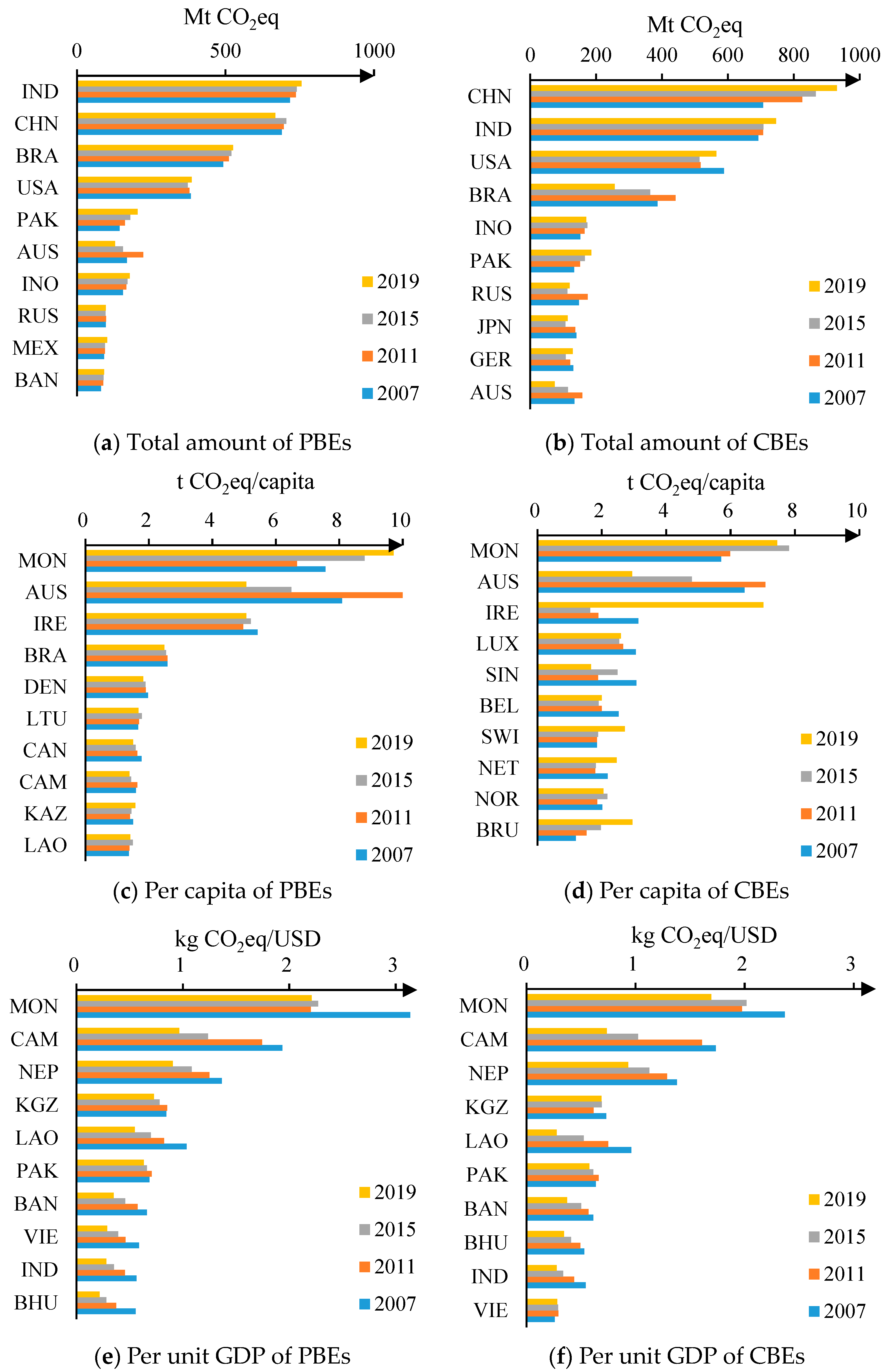
Figure 1 presents direct and embodied agricultural GHG emissions measured by the total amount, per capita, and per unit GDP. From 2007 to 2019, the direct emissions of agricultural GHG from the production perspective (PBEs) showed an upward trend, increasing from 3960.90 Mt CO2eq to 4091.15 Mt CO2eq at an average annual increase of 0.27%. In the same period, the consumption-based agricultural GHG emissions (CBEs) increased from 4555.48 Mt CO2eq to 4617.71 Mt CO2eq, averaging a 0.11% annual increase. Even though the PBEs’ growth rate surpassed the CBEs by 2.39 times, the overall volume of PBEs has always remained lower than that of CBEs in agriculture. When compared, the gap between consumption and production narrowed from 594.58 Mt CO2eq in 2007 to 526.56 Mt CO2eq in 2019.
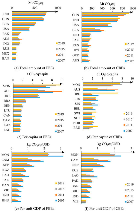
Figure 1.
The total amount (Mt CO2eq), per capita (t CO2eq/capita), and unit GDP (kg CO2eq/USD) of PBEs and CBEs in agricultural GHG emissions from 2007 to 2019 in order from bottom to top.
In PBEs, India, China, Brazil, and the United States rank among the highest. In 2007, as a large agricultural country, India’s agricultural GHG emissions reached 716.50 Mt CO2eq, representing 18.09% of the worldwide total. By 2019, the agricultural GHG emissions in India increased to 755.53 Mt CO2eq, comprising 18.47% of total agricultural emissions. China distinguished itself among the top five largest emitters in 2019 by experiencing a decrease in PBEs at a −0.28% average rate annually. In contrast, Brazil consistently held the third position of PBEs, accounting for 12.42% and 12.85% of global agricultural GHG emissions in 2007 and 2019, respectively. Despite the annual growth rate of the United States below that of the global average, it still remained the fourth largest producer of PBEs.
From a consumption-based perspective, China, India, the United States, and Brazil continued to dominate, accounting for 52.12% of global CBEs in 2007, further increasing to 54.13% in 2019. Among them, China was the largest emitter of CBEs, growing at an annual expansion of 2.32%. India was also a significant contributor to CBEs, increasing from 15.20% to 16.16% of the global total, averaging a 0.63% annual rate. Conversely, the CBEs of the United States and Brazil experienced a decrease but still ranked third and fourth in 2019, followed by Pakistan and Indonesia, whose CBEs rose by 52.54 and 18.23 Mt CO2eq, respectively, at annual rates of 2.81% and 0.95%.
Aligned with national attributes, India and China, with the highest total GHG emissions, had low per capita GHG emissions. With the expansion of the population base, India’s per capita PBEs and CBEs showed a downward trend. With the adjustment of economic structure, China’s PBEs per capita decreased by 0.05 tCO2eq per capita from 2007 to 2019, while the CBEs per capita showed a reverse evolution trend, increasing by 0.12 tCO2eq per capita. In contrast, Australia, Brazil, and the United States had both large per capita GHG emissions and large total emissions. Due to the shale gas revolution, the per capita PBEs and CBEs in the United States declined, but it still ranked 13th in 2019 with 1.18 tCO2eq per capita PBEs, while for CBEs, it ranked 11th with 1.72 tCO2eq per capita.
Considering GHG emissions per unit of GDP, agricultural production and consumption are relatively inefficient in less-developed countries. Among them, Mongolia had the largest PBEs per unit of GDP, followed by Cambodia and Nepal. However, from 2007 to 2019, their PBEs per unit GDP showed a downward trend. More specifically, Cambodia showed the most significant decline of 0.97 kg CO2eq/USD, followed by Mongolia, Laos, and Nepal, with declines of 0.93, 0.49, and 0.46 kg CO2eq/USD, respectively. Simultaneously, the CBEs per unit of GDP showed a similar pattern and evolution. The efficiency of agricultural consumption has also shown improvements in less developed regions, such as South Asia and Southeast Asia.
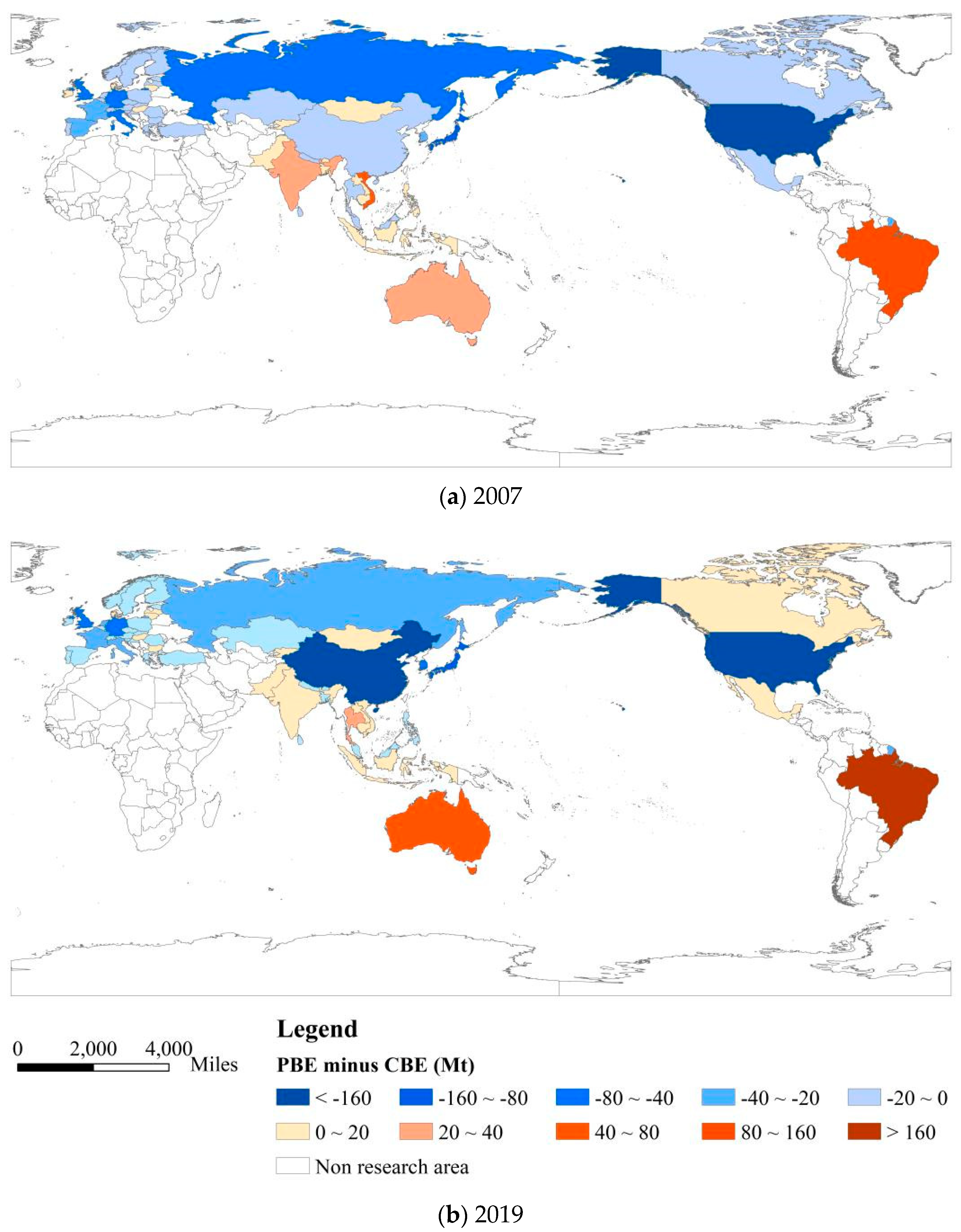
Figure 2 presents the differences between PBEs and CBEs by geographical distribution. Countries like the United States, Japan, China, the United Kingdom, and Germany, with considerable CBEs, address a larger loading portion for GHG emissions in agricultural consumption, while Brazil, Australia, Thailand, and India assume more loading for PBEs in agricultural GHG emissions. In 2007, the CBEs of the United States were 205.43 Mt CO2eq higher than the PBEs, with a gap that narrowed to 178.62 Mt CO2eq by 2019. Interestingly, China’s PBEs and CBEs in agricultural GHG were relatively balanced in 2007, while the difference, i.e., PBEs excess CBEs, rapidly climbed from −16.73 to −263.71 Mt CO2eq in 2019. The huge gap shows that China has increased its emphasis on the agricultural consumption side, achieved via international agricultural trade, as the growth rate of CBEs is much higher than that of PBEs by 2.60%.
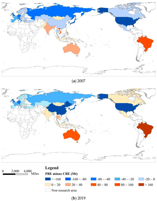
Figure 2.
Geographical distribution of differences between PBEs and CBEs in countries and regions from 2007 to 2019 (Mt CO2eq).
As a major agricultural producer in the world, Brazil’s agricultural PBEs were 105.45 and 268.63 Mt CO2eq larger than CBEs in 2007 and 2019, respectively. This indicates that Brazil bears a major global GHG emission loading of agricultural production, with an increasing trend. Although the surplus of PBEs to CBEs in Australia was less than that in Brazil, the difference still reached 34.43 Mt CO2eq in 2007 and 53.98 Mt CO2eq in 2019. In addition, with the increase in CBEs, the difference between Vietnam and India was significantly reduced, but they still contribute more to GHG emissions in production than consumption. On the contrary, Russia, Italy, and Spain showed deficits in carbon emission—i.e., higher CBEs than PBEs—rather than surpluses—i.e., more PBEs than CBEs—even though their gaps were significantly narrowed with the decline in CBEs. Further, the CBEs of Thailand, Mexico, and Canada also experienced significant decreases, while their main GHG emission loadings shifted from the consumption side to the production side, while Ireland, Bangladesh, and the Philippines showed the opposite status.
4.2. Agricultural GHG Emission Network Evolution
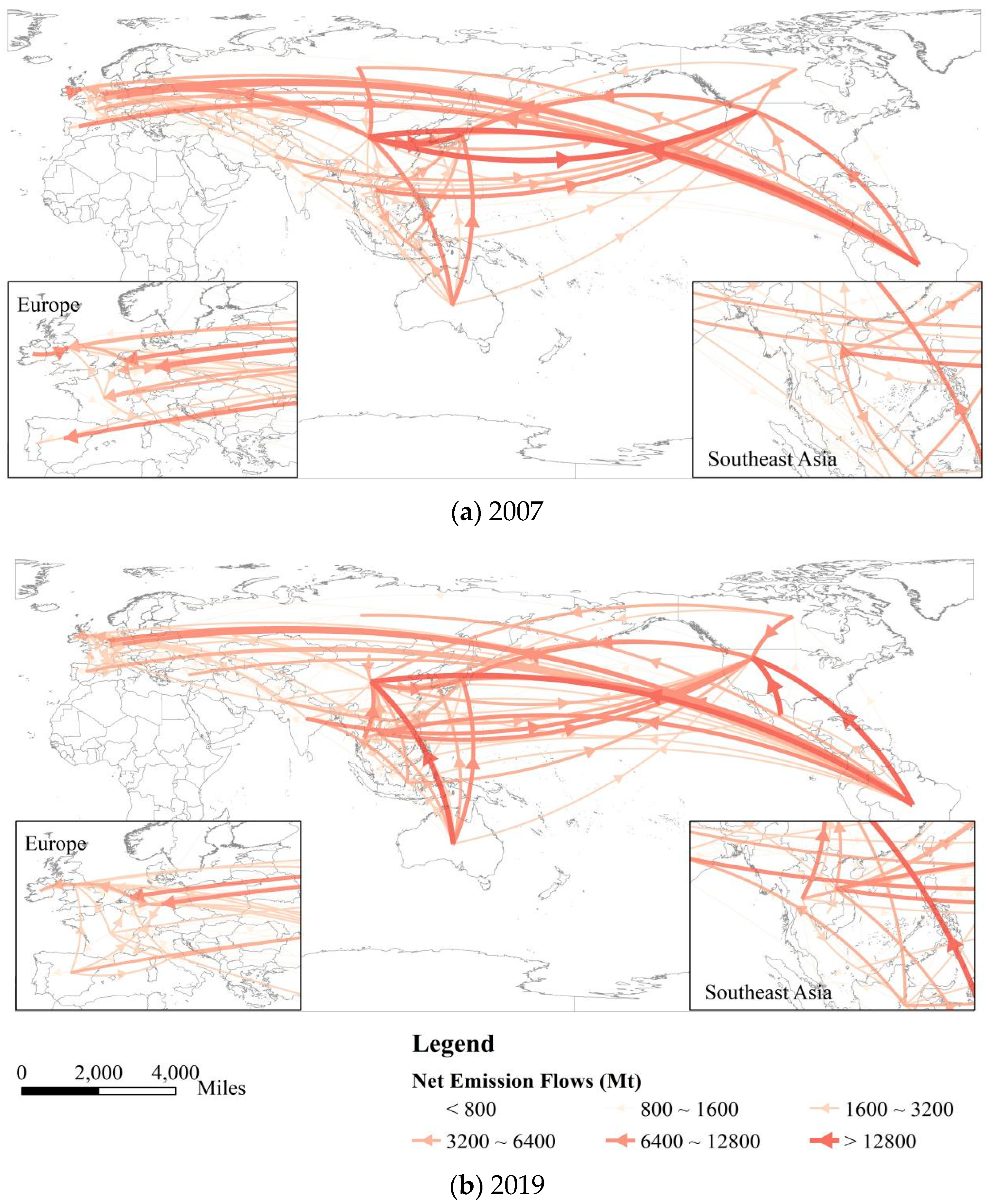
Figure 3 presents the global net flows of embodied agricultural GHG emissions worldwide. The total emissions experienced a rise, surging from 904,821.53 Mt CO2eq in 2007 to 1,367,875.01 Mt CO2eq in 2019, at an annual growth of 3.50%. This substantial increase in embodied GHG emissions surpassed the growth rates of both PBEs and CBEs, reflecting the significant impact of embodied emissions on global agricultural GHG patterns. Compared to the surface-level representations of PBEs and CBEs, these embodied emissions may encompass more extensive direct and indirect emissions that have frequently been overlooked.
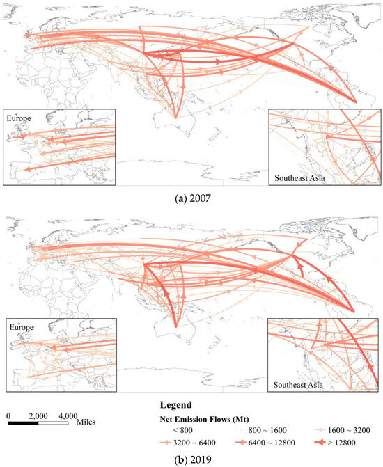
Figure 3.
Global net flows of embodied agricultural GHG emissions from 2007 to 2019 (Mt CO2eq). Note: the streamlines below 800 Mt CO2eq are not depicted in the figures.
As shown in Figure 3, Brazil emerged as the primary net outflow center, while the United States acted as the primary net inflow center for embodied agricultural GHG emissions. The global relationship between Brazil and China has been constantly developing for a long time. Simultaneously, the net flow patterns between Mexico and the United States, Australia and China, and Brazil and the United States became increasingly prominent, whereas China’s net emission exchanges with the United States and Japan showed a gradual reduction. As Brazil’s agricultural products trade, especially China’s dependence on Brazilian soybean imports, continued to expand, Brazil’s embodied agricultural GHG emissions to China significantly outweighed China’s emissions to Brazil. This considerable expansion of the net outflow scale from Brazil to China increased from 18,071.47 Mt CO2eq in 2007 to 141,945.27 Mt CO2eq in 2019, showing an annual growth rate of 18.74%.
Under the promotion of the North American Free Trade Agreement (NAFTA), agricultural commerce between the United States, Canada, and Mexico developed rapidly, leading to noticeable associated GHG emissions. The net outflow of embodied agricultural GHG from Mexico to the United States increased dramatically, from 4686.40 Mt CO2eq to 28,326.72 Mt CO2eq, becoming the second-largest net flow. As a consequence, Australia’s net flow of GHG emissions to China emerged as the third. The outflow scale of Brazil’s embodied agricultural GHG emissions to the United States ranked fourth in 2019 with a fluctuating overall trend. In the context of escalating trade friction, agricultural trade and the net flow scale between China and the United States have been negatively affected. Simultaneously, China’s net outflow to Japan dropped from second to seventh, with a reduction of 11,025.50 Mt CO2eq. However, the flows from Brazil to Vietnam and from Thailand to China saw a sharp rise in the emission scale in 2019, emerging as a significant global net flow.
4.3. Agricultural GHG Emission Network Characteristics
With the continuous strengthening of network correlations, the centrality of the embodied agricultural GHG emission network continues to decline, and the agglomeration characteristics decline in terms of the flow scale. The correlations among network nodes have been observed, signifying the growing participation of countries in global agricultural trade networks and agricultural GHG emissions. Meanwhile, network density increased, indicating closer linkages within the global emission network and increasing embodied emissions alongside the global flow of agricultural factors.
The changes in embodied emission networks are complex. On the one hand, the decreasing centralization suggests the ongoing weakening in high-value agglomeration characteristics among core nodes, contributing to a more balanced distribution of the network scale and a relaxation in the previously highly concentrated emission pattern. Among them, the embodied agricultural GHG emission network gradually shifted from being more affected on the export side than the import side, as the out-degree centralization of the network was smaller than the in-degree centralization since 2011. On the other hand, the ascendancy of core nodes in the embodied GHG emissions network increased, as evident in the increased network betweenness centralization. This enhancement indicated an increased ability to control essential nodes in the network. During the same period, network eigenvector centralization increased yearly, indicating increased interconnection between dominant nodes within the network structure.
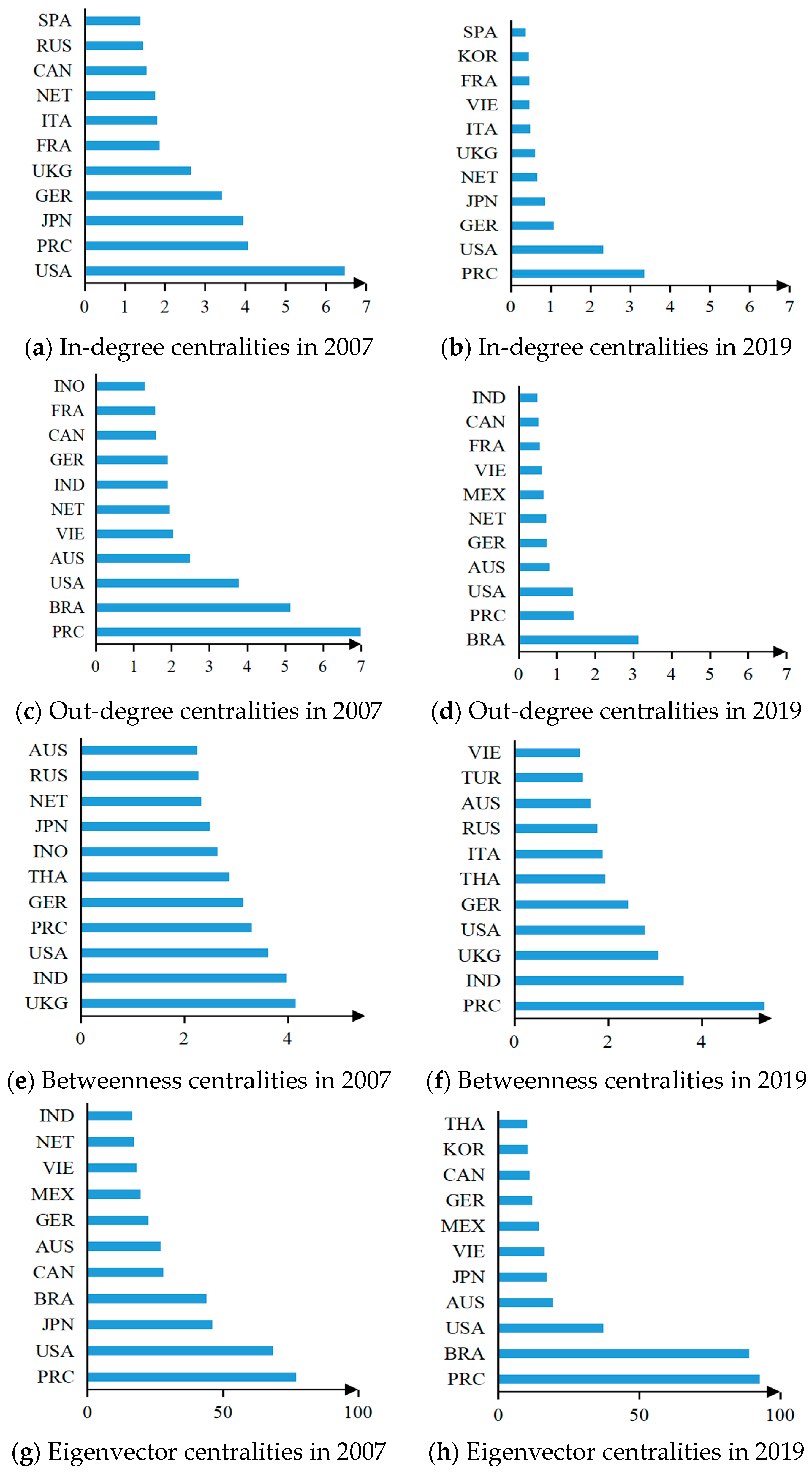
Figure 4 presents the embodied agricultural GHG emission network characteristics from 2007 to 2019. Regarding standardized weighted degree centralities, China, Brazil, the US, and Australia occupied dominant positions in out-degree centralities, whereas China, the United States, Germany, and Japan showed strong in-degree centralities. From the perspective of a decrease in out-degree, China’s local centrality declined to the most significant extent, succeeded by Australia, the United States, and Brazil, recording annual growth rates of −12.32%, −9.02%, −7.78%, and −4.08%, respectively. Meanwhile, China also experienced a marginal decrease in in-degree centrality, but it still overtook the United States as the primary hub for inflow convergence. Japan and Germany also showed scattered trends in the concentration of inflow, following the United States, with the most significant decline in centrality.
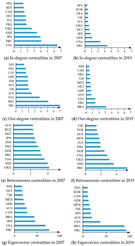
Figure 4.
Embodied agricultural GHG emission network characteristics from 2007 to 2019.
As shown by betweenness proportions, the United Kingdom, India, the United States, China, and Germany were more likely to act as intermediaries between other countries in streamlining agricultural emissions. In 2007, the United Kingdom’s potential to act as a vital node along the flow paths was 1.04, 1.15, 1.25, and 1.32 times that of India, the United States, China, and Germany. In 2019, China’s intermediary ability surpassed the United Kingdom’s in influencing the flow structure of pair paths. Moreover, Russia, Australia, Italy, and Turkey also showed relative improvements in their roles as emerging intermediate nodes, reflecting the enhancements in their bridging functions.
For the standardized symmetric eigenvector centralities, China, the United States, Japan, Brazil, and Australia held a prolonged dual advantage regarding the number and importance of adjacent nodes, consolidating their network influence through robust cooperation circles. Among them, China had the closest connectiveness with the most core countries, as its eigenvector centrality increased from 77.04% to 92.62%, maintaining the central position in the network. Simultaneously, Brazil notably increased its eigenvector centrality, growing from 44.04% in 2007 to 88.91% in 2019, while the United States, Japan, and Canada experienced substantial declines in their cooperation circle with other vital nodes.
4.4. Agricultural GHG Emission Network Clusters
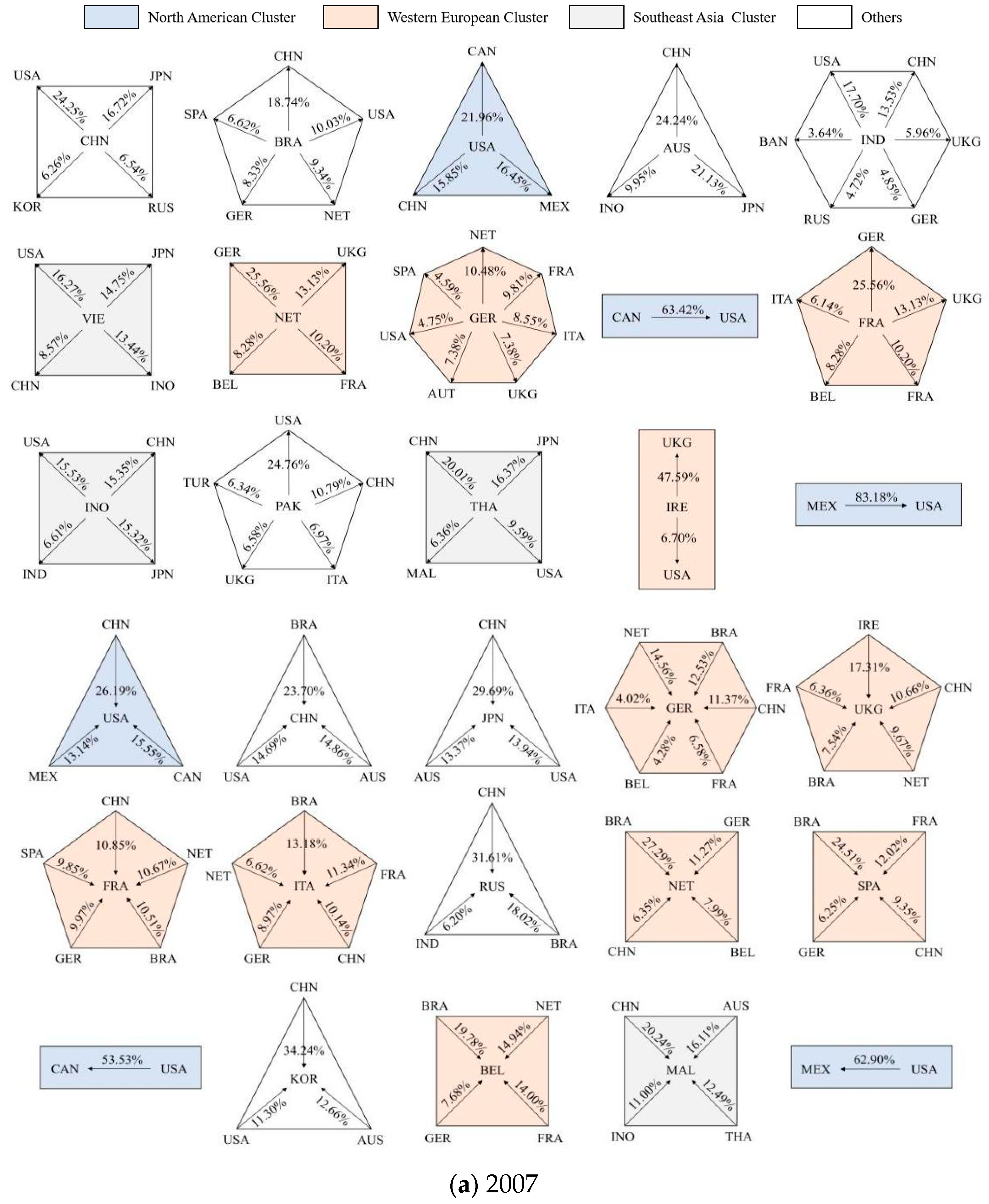
Figure 5 presents the embodied agricultural GHG clusters measured by outflows and inflows in 2007 and 2019. Regarding the agricultural GHG outflows, Canada, Mexico, and the United States formed an internal cluster in North America. Simultaneously, the Netherlands, Germany, and France remained core members of the Western European cluster, displaying a relatively balanced pattern for European countries but with reduced concentrations in 2019. In contrast, Ireland’s pattern was more concentrated, especially its outflows to the United Kingdom in 2007. With a decline in the scale of Irish outflows in 2019, Spain and the United Kingdom both increased their positions in the European cluster. In the Southeast Asia cluster, Vietnam, Indonesia, and Thailand exhibited close ties with other Asian countries, which have different evolutionary relationships with East Asia, Southeast Asia, and North America in 2019. In addition, the regional cluster characteristics in China, Brazil, Australia, India, and Pakistan were not evident in 2007, and their main outflows were not limited within their regions. However, Brazil and Australia’s balanced connection in agricultural GHG emissions was broken in 2019.
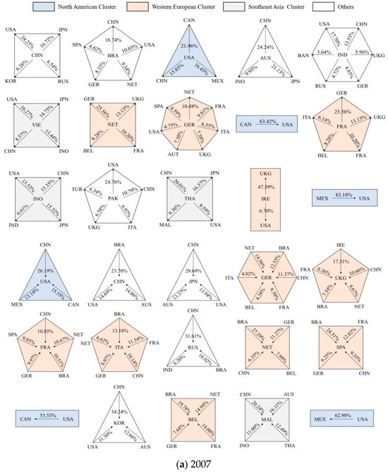
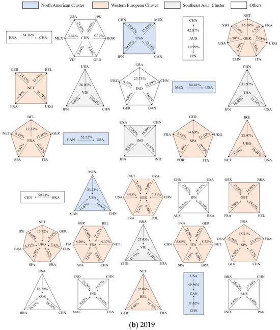
Figure 5.
Embodied agricultural GHG clusters by outflows and inflows in 2007 and 2019.
For the agricultural GHG inflows, the North American cluster remained significant. Yet the inflow dynamics within Canada and Mexico were dominated by the United States, which showed a relative weakening compared to the cluster pattern in 2007. Secondly, the inflow pattern formed a broader European cluster, including Germany, France, and the Netherlands as significant nodes. Further, countries like the United Kingdom, Italy, Spain, and Belgium were part of this cluster, strengthening internal relations within Europe to varying degrees in 2019. Traditional members of the Southeast Asian cluster, such as Indonesia, Malaysia, and Thailand, experienced declines in internal mobility within the group. In addition, Vietnam’s agricultural GHG inflow in the Southeast Asian cluster has gradually increased, with 40.30% of its emission inflow in 2019 originating from Asian countries, including China, Cambodia, Thailand, and India. Moreover, the diversity of China’s agricultural GHG inflows weakened, whereas Japan, South Korea, India, and Russia maintained relatively balanced global interconnection.
5. Discussion
To promote agricultural emission reduction and carbon neutrality achievement, several countries have implemented plans and measures [61,62,63]. The European Union, in 2020, introduced the European Green Deal and the European Climate Law, establishing a carbon neutrality goal for 2050 and outlining an overall framework and action steps for the European green development strategy. Similarly, New Zealand passed the Zero Carbon Bill in 2019, mandating a reduction in animal GHG emissions, except methane, to zero by 2050. The Climate Change Act of the United Kingdom has been in effect since 2008, further revised in June 2019, formally setting the nation’s aim for net-zero emissions by 2050. The United States reversed its downward trend in GHG emissions after withdrawing from the Paris Agreement in 2017. In contrast, since China’s National Programme for Climate Change was formulated in 2007, China’s embodied agricultural GHG emissions have generally shown negative growth, with an annual growth rate of −1.21% from 2007 to 2019. Table 2 demonstrates that different research scopes may yield different clustering outcomes. Related past research explored various methods, including community partitioning, k-means and hierarchical clustering, deep learning models, and spatial clustering analysis. Different cluster analysis methods, including community partitioning with the Girvan–Newman algorithm, block model, k-core, n-clan, k-plex, n-cliques, component analysis, lambda set method, and faction analysis were tested, contributing to descriptive statistics in assessing the composition of agricultural GHG emission flows in major countries and regions. Nonetheless, cluster analysis continues to be a valuable instrument for deepening the comprehension of correlations and positions among nations. Unlike descriptive statistical analysis, the block model method combines sub-regions such as Asia and North America into a single Asia-Pacific cluster, which is not conducive to subsequent analysis.
Table 2.
Comparisons between different clusters of agricultural GHG emissions.
The level of participation in international agricultural trade varies significantly. The diversity in strategies for achieving carbon peak and carbon neutrality is broad, stemming from the stark disparities of economic, social, political, cultural, and geographical aspects across countries and regions. Considering these differences, it is essential to tailor emission reduction goals, measures, paths, and policies to different clusters based on principles of equal rights and responsibilities, tolerance of differences, and win–win cooperation [68,69]. For internal clusters, the implementation of coordinated emission reduction strategies within the cluster could be strengthened. This approach will not only improve the inclusivity of emission reduction policies across different regions but also the applicability of relevant experiences, technology, and knowledge aspects.
Leveraging NAFTA and the United States–Mexico–Canada Agreement (USMCA), the North American cluster can improve the regional agricultural division of labor and capitalize on the technological advantages of the United States, thereby diminishing emissions associated with regional agricultural production. Further, the Western European cluster can take advantage of the integration organization of the EU, conducive to providing stringent rules, standards, and guarantees to effectively reduce regional GHG emissions. The Southeast Asian Cluster, under the framework of the Association of Southeast Asian Nations (ASEAN) and the Regional Comprehensive Economic Partnership (RCEP), can form a joint force to reduce agricultural emissions. According to the Law of Comparative Advantage, this strategy can facilitate countries with lower GHG emissions in agricultural production to export more low-carbon products, thereby alleviating local environmental pressure through agricultural trade by reducing the excessive production processes in inefficient countries.
However, measures to reduce agricultural GHG emissions through international trade may yield both potential synergies and tradeoffs [70]. For example, international trade based on comparative advantage may also affect the livelihoods of local actors engaged in agricultural production. Specialized production driven by international trade may result in a monolithic structure of local land use in the long term, affecting the richness of food structures. Simultaneously, addressing structural challenges such as power imbalances, vested interests, and fragmented policymaking requires effective communication platforms and consultation mechanisms for carbon emissions and transfer among multiple countries and regions.
The contribution of international trade to reducing agricultural emissions might be limited. The above analysis indicates that GHG emission flows are significantly affected by geopolitics, trade agreements, and international markets. While agricultural carbon emissions affect the global climate, global warming in turn will also affect its trade networks. The competitive nature and strategic trade-offs in the food trade market have led to large volatility in agricultural GHG emissions and could affect the orderly realization of emission reduction goals. Given the unique nature, periodicity, and strategy involved in agricultural activities, the practical environment often does not align with the optimal conditions for the division of labor and transactions as envisioned by comparative advantage theory. The combination may also require a diverse perspective, such as renewable energy and electrification, technological innovation, and the rationalization of the governance system. Among them, electrification can serve as an industrial chain solution to reduce carbon emissions. On the one hand, it helps to reduce the consumption of traditional fossil fuels and improve the utilization of the production efficiency of clean energy during agricultural production activities. On the other hand, it lays a low-carbon foundation for agricultural systems, including processing, packaging, transportation, and storage, through intelligent and automated technological updates.
In future studies, it is necessary to focus on the influencing factors and their mechanisms for agricultural GHG emissions in order to break through the limitations of existing research that focus on the patterns and drivers of GHG emissions. Secondly, it would be practical to explore how carbon emission reduction agreements (CERA) promote international agricultural cooperation to reduce overall GHG emissions, whether such agreements will lead to potential GHG emission deflection and crowding, and whether joint improvement in carbon emission efficiency can be achieved through technology transfer and diffusion. Additionally, it is essential to explore how different entities such as international organizations, countries, enterprises, and society react and weigh these influencing factors and whether there are interactions between these factors that generate new effects. Finally, reasonable emission reduction targets, strategies, and pathways could be compared and determined based on the strength, direction, and interaction from a multi-perspective viewpoint.
6. Conclusions
Employing multi-regional input–output modeling and complex network analysis, this study explores how embodied agricultural GHG emissions can be reflected and how they can tele-connect with the global agricultural trade network, especially focusing on Asia and the Pacific countries. Both PBEs and CBEs are on an upward trend, with the former increasing from 3960.90 to 4091.15 Mt CO2eq and the latter increasing from 4555.48 to 4617.71 Mt CO2eq. Notably, the most significant net emissions are recorded in trade routes from Brazil to China, the United States to China, and from Mexico to the United States, which reflects that agricultural trade can indeed have a temporal and spatial impact on GHG emission patterns via tele-connections. Despite an increase in connections and network density, the emission networks exhibited reduced agglomeration characteristics regarding both degree centralizations. Nevertheless, the core nodes continued to strengthen their leading roles, as evidenced by the betweenness and eigenvector centralization. The United Kingdom, India, the United States, China, and Germany functioned as network intermediaries, and China, the United States, Japan, Brazil, and Australia were also crucial for the number and significance of adjacent relations.
Certain economies show clear regional cluster characteristics in North America, Western Europe, and Southeast Asia. Compared to 2007, the North American cluster, made up of the United States, Canada, and Mexico, shows enhanced extraterritorial outflows and weakened extraterritorial inflows. The Western European cluster included the Netherlands, Germany, France, and Ireland, among others, demonstrating outflow diffusion and strengthened inflows within this region. The core members of the Southeast Asian cluster strengthened their connections with North American, East Asian, and South Asian countries in terms of agricultural GHG outflows, whereas the traditional core members strengthened their connections with extraterritorial countries in inflows. Some nodes previously had global linkages but gradually turned to a relationship with a small number of core countries. This shift has prompted the agricultural GHG emission network to remain influenced by the global core nodes. By linking embodied GHG emissions with the agricultural trade network, this study performs a practical framework in visualizing and quantifying environmental footprints by tele-connecting production and consumption sides and mapping GHG emissions permeating trade activities worldwide.
Supplementary Materials
The following supporting information can be downloaded at: https://www.mdpi.com/article/10.3390/land13122106/s1.
Author Contributions
Conceptualization, Z.S. and M.H.; methodology, J.G.; formal analysis, J.G.; writing—original draft preparation, Z.S. and J.G.; writing—review and editing, M.H. All authors have read and agreed to the published version of the manuscript.
Funding
This research was funded by the National Social Science Foundation of China (Grant no. 22CJY020), and the National Natural Science Foundation of China (Grant no. 72441005).
Data Availability Statement
The raw data supporting the conclusions of this article will be made available by the authors on request.
Conflicts of Interest
The authors declare no conflicts of interest.
References
- Climate Watch; World Resources Institute: Washington, DC, USA, 2022; Available online: https://www.climatewatchdata.org (accessed on 21 November 2023).
- Norse, D. Low carbon agriculture: Objectives and policy pathways. Environ. Dev. 2012, 1, 25–39. [Google Scholar] [CrossRef]
- Zang, D.G.; Hu, Z.J.; Yang, Y.Q.; He, S.Y. Research on the relationship between agricultural carbon emission intensity, agricultural economic development and agricultural trade in China. Sustainability 2022, 14, 11694. [Google Scholar] [CrossRef]
- De Pinto, A.; Li, M.; Haruna, A.; Hyman, G.G.; Martinez, M.A.L.; Creamer, B.; Kwon, H.-Y.; Garcia, J.B.V.; Tapasco, J.; Martinez, J.D. Low Emission Development Strategies in Agriculture. An Agriculture, Forestry, and Other Land Uses (AFOLU) Perspective. World Dev. 2016, 87, 180–203. [Google Scholar] [CrossRef]
- Lee, J.H.; Woo, J. Green New Deal Policy of South Korea: Policy Innovation for a Sustainability Transition. Sustainability 2020, 12, 10191. [Google Scholar] [CrossRef]
- Kim, C.G. The Impact of Climate Change on the Agricultural Sector: Implications of the Agro-Industry for Low Carbon, Green Growth Strategy and Roadmap for the East Asian Region. Low Carbon Green Growth Roadmap for Asia and the Pacific. 2012. Available online: https://hdl.handle.net/20.500.12870/4032 (accessed on 21 June 2024).
- Piwowar, A. Low-carbon agriculture in Poland: Theoretical and practical challenges. Pol. J. Environ. Stud. 2019, 28, 2785–2792. [Google Scholar] [CrossRef]
- Gołasa, P.; Wysokiński, M.; Bieńkowska-Gołasa, W.; Gradziuk, P.; Golonko, M.; Gradziuk, B.; Siedlecka, A.; Gromada, A. Sources of Greenhouse Gas Emissions in Agriculture, with Particular Emphasis on Emissions from Energy Used. Energies 2021, 14, 3784. [Google Scholar] [CrossRef]
- Rebolledo-Leiva, R.; Angulo-Meza, L.; Iriarte, A.; Gonzalez-Araya, M.C. Joint carbon footprint assessment and data envelopment analysis for the reduction of greenhouse gas emissions in agriculture production. Sci. Total Environ. 2017, 593, 36–46. [Google Scholar] [CrossRef]
- Drabo, A. Climate change mitigation and agricultural development models: Primary commodity exports or local consumption production? Ecol. Econ. 2017, 137, 110–125. [Google Scholar] [CrossRef]
- Yu, Y.; Jiang, T.Y.; Li, S.Q.; Li, X.L.; Gao, D.C. Energy-related CO2 emissions and structural emissions’ reduction in China’s agriculture: An input-output perspective. J. Clean. Prod. 2020, 276, 124169. [Google Scholar] [CrossRef]
- Han, M.Y.; Lao, J.M.; Yao, Q.H.; Zhang, B.; Meng, J. Carbon Inequality and Economic Development Across the Belt and Road Regions. J. Environ. Manag. 2020, 262, 110250. Available online: https://www.sciencedirect.com/science/article/pii/S0301479720301857 (accessed on 15 August 2024). [CrossRef]
- Niu, B.B.; Peng, S.; Li, C.; Liang, Q.; Li, X.J.; Wang, Z. Nexus of embodied land use and greenhouse gas emissions in global agricultural trade: A quasi-input-output analysis. J. Clean. Prod. 2020, 267, 122067. [Google Scholar] [CrossRef]
- Bajan, B.; Mrówczyńska-Kamińska, A. Carbon footprint and environmental performance of agribusiness production in selected countries around the world. J. Clean. Prod. 2020, 276, 123389. [Google Scholar] [CrossRef]
- Dace, E.; Blumberga, D. How do 28 European Union Member States perform in agricultural greenhouse gas emissions? It depends on what we look at: Application of the multi-criteria analysis. Ecol. Indic. 2016, 71, 352–358. [Google Scholar] [CrossRef]
- Flysjö, A.; Henriksson, M.; Cederberg, C.; Ledgard, S.; Englund, J.E. The impact of various parameters on the carbon footprint of milk production in New Zealand and Sweden. Agric. Syst. 2011, 104, 459–469. [Google Scholar] [CrossRef]
- Thoma, G.; Popp, J.; Nutter, D.; Shonnard, D.; Ulrich, R.; Matlock, M.; Kim, D.S.; Neiderman, Z.; Kemper, N.; East, C.; et al. Greenhouse gas emissions from milk production and consumption in the United States: A cradle-to-grave life cycle assessment circa 2008. Int. Dairy J. 2013, 31, S3–S14. [Google Scholar] [CrossRef]
- Wojcik-Gront, E.; Bloch-Michalik, M. Assessment of greenhouse gas emission from life cycle of basic cereals production in Poland. Zemdirb.-Agric. 2016, 103, 259–266. [Google Scholar] [CrossRef]
- Zhang, G.S.; Wang, S.S. China’s agricultural carbon emission: Structure, efficiency and its determinants. Issues Agric. Econ. 2014, 35, 18–26+110. (In Chinese) [Google Scholar] [CrossRef]
- Beauchemin, K.A.; Henry Janzen, H.; Little, S.M.; McAllister, T.A.; McGinn, S.M. Life cycle assessment of greenhouse gas emissions from beef production in western Canada: A case study. Agric. Syst. 2010, 103, 371–379. [Google Scholar] [CrossRef]
- da Silva, V.P.; van der Werf, H.M.G.; Spies, A.; Soares, S.R. Variability in environmental impacts of Brazilian soybean according to crop production and transport scenarios. J. Environ. Manag. 2010, 91, 1831–1839. [Google Scholar] [CrossRef]
- Farag, A.A.; Abd-Elrahman, S.H. Greenhouse gas emission from cauliflower grown under different nitrogen rates and mulches. Int. J. Soil Sci. 2016, 9, 1–10. [Google Scholar] [CrossRef]
- Huang, X.Q.; Xu, X.C.; Wang, Q.Q.; Zhang, L.; Gao, X.; Chen, L.H. Assessment of agricultural carbon emissions and their spatiotemporal changes in China, 1997-2016. Int. J. Environ. Res. Public Health 2019, 16, 3105. [Google Scholar] [CrossRef] [PubMed]
- Qiu, Z.J.; Jin, H.M.; Gao, N.; Xun, X.; Zhu, J.H.; Li, Q.; Wang, Z.Q.; Xun, Y.J.; Shen, W.S. Temporal characteristics and trend prediction of agricultural carbon emission in Jiangsu Province, China. J. Agro-Environ. Sci. 2022, 41, 658–669. (In Chinese) [Google Scholar] [CrossRef]
- Zhou, S.Y.; Xi, F.M.; Yin, Y.; Bing, L.F.; Wang, J.Y.; Ma, M.J.; Zhang, W.F. Accounting and drivers of carbon emission from cultivated land utilization in Northeast China. Chin. J. Appl. Ecol. 2021, 32, 3865–3871. (In Chinese) [Google Scholar] [CrossRef]
- Song, K.H.; Baiocchi, G.; Feng, K.S.; Hubacek, K.; Sun, L.X.; Wang, D.P.; Guan, D.B. Can U.S. multi-state climate mitigation agreements work? A perspective from embedded emission flows. Global Environ. Change 2022, 77, 102596. [Google Scholar] [CrossRef]
- Yun, T.; Zhang, J.B.; He, Y.Y. Research on Spatial-Temporal Characteristics and Driving Factor of Agricultural Carbon Emissions in China. J. Integr. Agric. 2014, 13, 1393–1403. [Google Scholar] [CrossRef]
- Garnier, J.; Le Noe, J.; Marescaux, A.; Sanz-Cobena, A.; Lassaletta, L.; Silvestre, M.; Thieu, V.; Billen, G. Long-term changes in greenhouse gas emissions from French agriculture and livestock (1852–2014): From traditional agriculture to conventional intensive systems. Sci. Total Environ. 2019, 660, 1486–1501. [Google Scholar] [CrossRef]
- Hellweg, S.; Milà i Canals, L. Emerging approaches, challenges and opportunities in life cycle assessment. Science 2014, 344, 1109–1113. [Google Scholar] [CrossRef]
- Rebitzer, G.; Ekvall, T.; Frischknecht, R.; Hunkeler, D.; Norris, G.; Rydberg, T.; Schmidt, W.-P.; Suh, S.; Weidema, B.P.; Pennington, D.W. Life cycle assessment part 1: Framework, goal and scope definition, inventory analysis, and applications. Environ. Int. 2004, 30, 701–720. [Google Scholar] [CrossRef]
- Du, J.; Luo, J.; Wang, R.; Wang, X.H. The estimation and analysis of spatio-temporal change patterns of carbon functions in major grain producing area. J. Ecol. Rural. Environ. 2019, 35, 1242–1251. (In Chinese) [Google Scholar] [CrossRef]
- Xia, L.L.; Ti, C.P.; Li, B.L.; Xia, Y.Q.; Yan, X.Y. Greenhouse gas emissions and reactive nitrogen releases during the life-cycles of staple food production in China and their mitigation potential. Sci. Total Environ. 2016, 556, 116–125. [Google Scholar] [CrossRef]
- Wang, X.Z.; Liu, B.; Wu, G.; Sun, Y.X.; Guo, X.S.; Jin, Z.H.; Xu, W.N.; Zhao, Y.Z.; Zhang, F.S.; Zou, C.Q.; et al. Environmental costs and mitigation potential in plastic-greenhouse pepper production system in China: A life cycle assessment. Agric. Syst. 2018, 167, 186–194. [Google Scholar] [CrossRef]
- Matthews, H.S.; Hendrickson, C.T.; Weber, C.L. The importance of carbon footprint estimation boundaries. Environ. Sci. Technol. 2008, 42, 5839–5842. [Google Scholar] [CrossRef] [PubMed]
- Pandey, D.; Agrawal, M. Carbon Footprint Estimation in the Agriculture Sector. In Assessment of Carbon Footprint in Different Industrial Sectors; Muthu, S.S., Ed.; Springer: Singapore, 2014; Volume 1, pp. 25–47. [Google Scholar]
- Sheng, X.R.; Chen, L.P.; Liu, M.Y.; Wang, Q.S.; Ma, Q.; Zuo, J.; Yuan, X.L. Input-output models for carbon accounting: A multi-perspective analysis. Renew. Sustain. Energy Rev. 2025, 207, 114950. [Google Scholar] [CrossRef]
- Cicas, G.; Hendrickson, C.T.; Horvath, A.; Matthews, H.S. A regional version of a US economic input-output life-cycle assessment model. Int. J. Life Cycle Assess. 2007, 12, 365–372. [Google Scholar] [CrossRef]
- Wiedmann, T. A review of recent multi-region input–output models used for consumption-based emission and resource accounting. Ecol. Econ. 2009, 69, 211–222. [Google Scholar] [CrossRef]
- Wiedmann, T.; Wilting, H.C.; Lenzen, M.; Lutter, S.; Palm, V. Quo Vadis MRIO? Methodological, data and institutional requirements for multi-region input–output analysis. Ecol. Econ. 2011, 70, 1937–1945. [Google Scholar] [CrossRef]
- Han, M.Y.; Zhang, B.; Zhang, Y.Q.; Guan, C.H. Agricultural CH4 and N2O Emissions of Major Economies: Consumption-vs. Production-Based Perspectives. J. Clean. Prod. 2019, 210, 276–286. Available online: https://www.sciencedirect.com/science/article/pii/S0959652618334188 (accessed on 21 May 2024). [CrossRef]
- Sun, X.D.; Li, Z.Y.; Cheng, X.L.; Guan, C.H.; Han, M.Y.; Zhang, B. Global Anthropogenic CH4 Emissions from 1970 to 2018: Gravity Movement and Decoupling Evolution. Resour. Conserv. Recycl. 2022, 182, 106335. Available online: https://www.sciencedirect.com/science/article/pii/S0921344922001811 (accessed on 18 May 2024). [CrossRef]
- Yan, C.H.; Han, M.Y.; Liu, Y.; Zhang, B. Household CH4 and N2O Footprints of Major Economies. Earth’s Future 2021, 9, e2021EF002143. Available online: https://agupubs.onlinelibrary.wiley.com/doi/10.1029/2021EF002143 (accessed on 1 June 2024). [CrossRef]
- Guo, J.; Zhang, Y.J.; Zhang, K.B. The key sectors for energy conservation and carbon emissions reduction in China: Evidence from the input-output method. J. Clean. Prod. 2018, 179, 180–190. [Google Scholar] [CrossRef]
- Su, B.; Ang, B.W.; Li, Y.Z. Input-output and structural decomposition analysis of Singapore’s carbon emissions. Energy Policy 2017, 105, 484–492. [Google Scholar] [CrossRef]
- Zhang, Q.F.; Fang, K.; Xu, M.; Liu, Q.Y. Review of carbon footprint research based on input-output analysis. J. Nat. Resour. 2018, 33, 696–708. (In Chinese) [Google Scholar] [CrossRef]
- Ji, X.; Han, M.Y.; Ulgiati, S. Optimal Allocation of Direct and Embodied Arable Land Associated to Urban Economy: Understanding the Options Deriving from Economic Globalization. Land Use Policy 2020, 91, 104392. Available online: https://www.sciencedirect.com/science/article/pii/S0264837719312463 (accessed on 21 June 2024). [CrossRef]
- Song, Z.Y.; Zhu, Q.L.; Han, M.Y. Tele-Connection of Global Crude Oil Network: Comparisons Between Direct Trade and Embodied Flows. Energy 2021, 217, 119359. Available online: https://www.sciencedirect.com/science/article/pii/S036054422032466X (accessed on 21 June 2024). [CrossRef]
- Zhang, X.L.; Tang, D.C.; Kong, S.Y.; Wang, X.L.; Xu, T.; Boamah, V. The carbon effects of the evolution of node status in the world trade network. Front. Environ. Sci. 2022, 10, 2027. [Google Scholar] [CrossRef]
- Tabassum, S.; Pereira, F.S.F.; Fernandes, S.; Gama, J. Social network analysis: An overview. WIREs Data Min. Knowl. Discov. 2018, 8, e1256. [Google Scholar] [CrossRef]
- Pace, M.L.; Gephart, J.A. Trade: A Driver of Present and Future Ecosystems. Ecosystems 2017, 20, 44–53. [Google Scholar] [CrossRef]
- Verburg, R.; Stehfest, E.; Woltjer, G.; Eickhout, B. The effect of agricultural trade liberalisation on land-use related greenhouse gas emissions. Glob. Environ. Chang. 2009, 19, 434–446. [Google Scholar] [CrossRef]
- He, Y.Q.; Lan, X.; Zhou, Z.A.; Wang, F. Analyzing the spatial network structure of agricultural greenhouse gases in China. Environ. Sci. Pollut. Res. 2021, 28, 7929–7944. [Google Scholar] [CrossRef]
- Qu, J.S.; Han, J.Y.; Liu, L.N.; Xu, L.; Li, H.J.; Fan, Y.J. Inter-provincial correlations of agricultural GHG emissions in China based on social network analysis methods. China Agric. Econ. Rev. 2020, 13, 229–246. [Google Scholar] [CrossRef]
- Yang, Z.F.; Mao, X.F.; Zhao, X.; Chen, B. Ecological network analysis on global virtual water trade. Environ. Sci. Technol. 2012, 46, 1796–1803. [Google Scholar] [CrossRef] [PubMed]
- Guan, J.; Song, Z.Y.; Liu, W.D. Change of the global grain trade network and its driving factors. Prog. Geogr. 2022, 41, 755–769. (In Chinese) [Google Scholar] [CrossRef]
- Li, Z.L.; Sun, L.; Geng, Y.; Dong, H.J.; Ren, J.Z.; Liu, Z.; Tian, X.; Yabar, H.; Higano, Y. Examining industrial structure changes and corresponding carbon emission reduction effect by combining input-output analysis and social network analysis: A comparison study of China and Japan. J. Clean. Prod. 2017, 162, 61–70. [Google Scholar] [CrossRef]
- He, Z.; Yang, Y.; Liu, Y.; Jin, F.J. Characteristics of evolution of global energy trading network and relationships between major countries. Prog. Geogr. 2019, 38, 1621–1632. (In Chinese) [Google Scholar] [CrossRef]
- FAO. FAOSTAT—Food and Agriculture Data. 2021. Available online: https://www.fao.org/faostat/en/#data/GT (accessed on 28 July 2023).
- Asian Development Bank. Input-Output Tables for Asia and the Pacific. Available online: https://www.adb.org/what-we-do/data/regional-input-output-tables (accessed on 12 November 2023).
- World Bank. World Bank Open Data 2022. Available online: https://data.worldbank.org.cn/indicator/SP.POP.TOTL (accessed on 12 November 2023).
- Huisingh, D.; Zhang, Z.H.; Moore, J.C.; Qiao, Q.; Li, Q. Recent advances in carbon emissions reduction: Policies, technologies, monitoring, assessment and modeling. J. Clean. Prod. 2015, 103, 1–12. [Google Scholar] [CrossRef]
- Fekete, H.; Kuramochi, T.; Roelfsema, M.; Den Elzen, M.; Forsell, N.; Höhne, N.; Luna, L.; Hans, F.; Sterl, S.; Olivier, J.; et al. A review of successful climate change mitigation policies in major emitting economies and the potential of global replication. Renew. Sustain. Energy Rev. 2021, 137, 110602. [Google Scholar] [CrossRef]
- Lamb, W.F.; Grubb, M.; Diluiso, F.; Minx, J.C. Countries with sustained greenhouse gas emissions reductions: An analysis of trends and progress by sector. Clim. Policy 2022, 22, 1–17. [Google Scholar] [CrossRef]
- Zhao, X.L.; Wu, X.F.; Guan, C.H.; Ma, R.; Nielsen, C.P.; Zhang, B. Linking Agricultural GHG Emissions to Global Trade Network. Earth’s Future 2020, 8, e2019EF001361. [Google Scholar] [CrossRef]
- Kolasa-Więcek, A. Neural Modeling of Greenhouse Gas Emission from Agricultural Sector in European Union Member Countries. Water Air Soil Pollut. 2018, 229, 1–12. [Google Scholar] [CrossRef]
- Pradhan, P.; Reusser, D.E.; Kropp, J.P. Embodied greenhouse gas emissions in diets. PLoS ONE 2013, 8, e62228. [Google Scholar] [CrossRef]
- Ghanbari, S.; Mansouri Daneshvar, M.R. Urban and rural contribution to the GHG emissions in the MECA countries. Environ. Dev. Sustain. 2021, 23, 6418–6452. [Google Scholar] [CrossRef]
- Osborn, D.; Cutter, A.; Ullah, F. Universal sustainable development goals: Understanding the transformational challenge for developed countries. Stakehold. Forum 2015, 2, 1–25. [Google Scholar]
- Vanderheiden, S. Common but differentiated responsibilities. In Essential Concepts of Global Environmental Governance; Routledge: London, UK, 2020; pp. 41–43. [Google Scholar]
- Zurek, M.; Hebinck, A.; Selomane, O. Climate Change and the Urgency to Transform Food Systems. Science 2022, 376, 1416–1421. Available online: https://www.science.org/doi/10.1126/science.abo2364 (accessed on 18 June 2024). [CrossRef] [PubMed]

Disclaimer/Publisher’s Note: The statements, opinions and data contained in all publications are solely those of the individual author(s) and contributor(s) and not of MDPI and/or the editor(s). MDPI and/or the editor(s) disclaim responsibility for any injury to people or property resulting from any ideas, methods, instructions or products referred to in the content. |
© 2024 by the authors. Licensee MDPI, Basel, Switzerland. This article is an open access article distributed under the terms and conditions of the Creative Commons Attribution (CC BY) license (https://creativecommons.org/licenses/by/4.0/).