Abstract
The complexity of urban street vitality is reflected in the interaction of multiple factors. A deep understanding of the multi-dimensional driving mechanisms behind it is crucial to enhancing urban street vitality. However, existing studies lack comprehensive interpretative analyses of urban multi-source data, making it difficult to uncover these drivers’ nonlinear relationships and interaction effects fully. This study introduces an interpretable machine learning framework, using Nanchang, China as a case study. It utilizes urban multi-source data to explore how these variables influence different dimensions of street vitality. This study’s innovation lies in employing an integrated measurement approach which reveals the complex nonlinearities and interaction effects between data, providing a more comprehensive explanation. The results not only demonstrate the strong explanatory power of the measurement approach but also reveal that (1) built environment indicators play a key role in influencing street vitality, showing significant spatial positive correlations; (2) different dimensions of street vitality exhibit nonlinear characteristics, with transit station density being the most influential one; and (3) cluster analysis revealed distinct built environment and socioeconomic characteristics across various street vitality types. This study provides urban planners with a data-driven quantitative tool to help formulate more effective strategies for enhancing street vitality.
1. Introduction
Urban streets are essential spaces for social, economic, and cultural activities, forming a vital component of urban public spaces [1]. Since the 1960s, urban planning has considered street vitality a key indicator of urban attractiveness and sustainable development potential [2,3]. Scholars from various disciplines have interpreted street vitality from different perspectives. Urban sociologists argue that economic, social, and cultural vitality intertwines with street vitality, representing these activities spatially [4]. Urban planners maintain that design and high-quality built environments can enhance vitality [5]. Thus, understanding the relationships among economic, social, cultural, and built environment factors is crucial for revealing the drivers and spatial distribution of street vitality, ultimately boosting urban vitality.
Research on urban street vitality has evolved through several phases. Early studies relied on field surveys to quantify street vitality, though these methods are time-consuming and not scalable [6]. Recent advances in deep learning and urban multi-source data have shifted the research paradigm, allowing for more comprehensive assessments of street vitality and its physical environment indicators [7,8]. Many studies have integrated multi-source data—such as street view images, points of interest, housing prices, and land use—along with advanced techniques like image classification and semantic segmentation to capture urban street vitality [9,10,11,12].
However, existing studies often consolidate various dimensions of street vitality—economic, social, and visual perception—into a single indicator, lacking differential analyses and explanations of factors influencing distinct types of street vitality. Specifically, current research primarily examines spatial factors like the built environment, with limited exploration of how urban multi-source data, such as natural elements, population density, housing prices, and facility richness, affect street vitality. Additionally, many studies rely on linear assumptions, failing to explore nonlinear impacts on urban street vitality. Interactions and threshold effects between various vitality types and their influencing factors remain underexplored [13,14,15,16,17,18].
To address these research limitations, this study proposes a comprehensive framework integrating multi-source big data and advanced machine learning methods to uncover the nonlinear and interactive effects of urban data on different dimensions of street vitality. The contributions of this study include (1) collecting various types of urban multi-source data as independent variables while combining different dimensions of street vitality—perceptual, social, and economic—as dependent variables, yielding a comprehensive understanding of street vitality and its influencing factors; (2) Employing Extreme Gradient Boosting (XGBoost) and SHapley Additive exPlanations (SHAP) models to elucidate the complex nonlinear impacts and interactions among natural elements, socioeconomic indicators, and built environment factors on different dimensions of street vitality; and (3) utilizing hierarchical clustering analysis to identify distinct vitality types of urban streets, providing urban planners with insights into localized the effect patterns of multi-source data to formulate targeted strategies for enhancing vitality and guiding redevelopment across different street types.
To overcome these limitations, this study develops a novel framework which integrates multi-source urban data with advanced machine learning techniques to investigate the nonlinear and interactive effects on different dimensions of street vitality. The key contributions are as follows. (1) We comprehensively incorporate diverse urban data, such as natural elements, population density, and facility richness, as independent variables while distinguishing between perceptual, social, and economic vitality as dependent variables. This allows for a more nuanced understanding of the factors driving each vitality type. (2) We apply Extreme Gradient Boosting (XGBoost) and SHapley Additive exPlanations (SHAP) to reveal the nonlinear relationships and interactions among natural, socioeconomic, and built environment factors, offering a detailed explanation of their complex impacts on street vitality. (3) Finally, hierarchical clustering is used to identify distinct street vitality patterns, providing targeted insights for urban planners to enhance vitality and guide redevelopment efforts tailored to specific street types. This research not only advances the methodological approach but also deepens the understanding of urban street dynamics, offering practical implications for sustainable urban development.
2. Related Works
2.1. Definition and Quantification of Urban Street Vitality
Urban vitality is a crucial factor reflecting urban competitiveness, yet scholars have proposed various definitions without a widely accepted standard. Jacobs introduced “eyes on the street”, asserting that land use mix and community permeability directly influence urban vitality [1]. Lynch identified three key elements: social dynamics, urban form, and functionality [19]. Montgomery defined vitality through pedestrian flow, facility usage, activity levels, and street vibrancy [20]. Thus, urban vitality is closely linked to human activity and streets, which serve as vital media for social and physical interactions.
Some scholars have approached urban street vitality from a macro perspective. Zijderveld viewed it as the spatial representation of economic, social, and cultural activities [4]. Most studies quantify urban street vitality through social and economic factors, as these intuitively reflect urban form and human activity intensity [16]. However, the quality of visual and spatial elements significantly influences how individuals perceive the urban atmosphere, with only a few studies considering visual perception data as an influencing factor [17,21].
2.2. Relationship Between Multi-Source Urban Data and Urban Street Vitality
Traditionally, studies gathered data through field surveys and questionnaires, quantifying urban street vitality via comparisons and expert ratings [22]. This approach is limited in scope, poses challenges for data acquisition, and fails to explain the degree of influence of various factors [23]. With advancements in theoretical research and the availability of multi-source big data, scholars have explored the relationships between various variables and urban street vitality from diverse perspectives. It is widely recognized that built environment factors, alongside social, economic, and demographic characteristics, significantly impact urban street vitality [7,15,16,24,25,26].
Built environment factors are typically categorized into “5D” categories: density, diversity, design, distance to transport, and destination accessibility. Meng et al. established a significant relationship between the 5D built environment and urban street vitality [9]. Huang et al. identified population density, building quality, and street walkability as key factors affecting street vitality in Shanghai [27]. Xia et al. confirmed a positive spatial autocorrelation between land development intensity and street vitality using data from small restaurants and nighttime lighting [28]. Additionally, research has examined the relationships between network accessibility [24], service facilities [29], and commercial density [7] with urban street vitality.
On the other hand, urban street vitality emphasizes the relationship between human activity and urban space, with socioeconomic indicators reflecting human activity intensity, which correlates highly with street vitality. Jia et al. developed a multiple regression model linking urban economic landscapes to street vitality, confirming their correlation [30]. Factors such as housing prices, population density, nighttime lighting, GDP, and travel heat maps are also considered important for assessing street vitality [16,25,31,32]. However, research on the impact of natural elements on urban street vitality remains limited. This study incorporates natural elements alongside socioeconomic and built environment 5D indicators to explore the influence of multi-source data on urban street vitality.
At the same time, several studies have explored the temporal and spatial evolution of urban vitality and its driving factors. For example, Chen et al. used mobile phone data to reveal the differences in urban vitality patterns between weekdays and weekends as well as their spatiotemporal dynamics [33]. Xia et al. uncovered how the relationship between urban morphology and vitality fluctuates with the time and location throughout the day [34]. These studies provide valuable insights into the dynamic nature of urban vitality.
In this study, data for the variables were collected in 2022 to ensure consistency and comparability. The independent variables we selected, such as NDVI, population density, and GDP density, are mostly based on annual averages or relatively stable long-term data on buildings and roads, aiming to minimize the noise introduced by short-term fluctuations. Although this study does not involve temporal analysis, its primary goal is to reveal the relationship between urban vitality and these relatively stable variables, thereby understanding the driving factors of vitality through static indicators. This foundational research will lay the groundwork for future dynamic analyses.
2.3. Machine Learning Methods for Revealing Nonlinear Relationships and Interactions
Early studies on urban street vitality primarily employed linear regression models [7,11,35,36,37,38], which struggled to capture complex nonlinear relationships. With advancements in machine learning, researchers increasingly utilize these methods to analyze the relationships between variables and street vitality.
Among various machine learning techniques, gradient boosting decision trees (GBDT) are widely used for their efficiency and reliability [39]. For example, Yang et al. and Peng et al. employed GBDT to explore the nonlinear relationship between subway traffic and urban vitality [25,40]. XGBoost, an enhancement over GBDT, offers advantages in handling sparse and parallel data, significantly improving computational speeds [41]. Chang et al. and J. Liu et al. applied XGBoost to investigate the relationships between street environments and pedestrian accidents, as well as between built environments and traffic enthusiasm [30,42]. Z. Xiao et al. found that XGBoost outperformed traditional methods [43].
This study employs the SHAP model to assess the impact of independent variables on dependent variables, using Shapley values to provide equitable explanations. SHAP’s local interpretative capability often surpasses that of global methods [44,45]. Therefore, this study utilizes the SHAP model to interpret XGBoost results, analyzing the effects of various influencing factors on urban street vitality.
3. Methods and Datasets
The process of this study is illustrated in Figure 1, and it comprised four steps to investigate the impacts of urban multi-source data on street vitality: (1) data collection and indicator calculation; (2) modeling the relationship between multi-source data indicators and various dimensions of urban street vitality using the XGBoost model; (3) explaining the XGBoost model with SHAP to assess the nonlinear global and local impacts of multi-source data indicators on different dimensions of urban street vitality, as well as the interactions among key factors; and (4) classifying urban vitality types through clustering methods and analyzing street characteristics under different vitality categories.
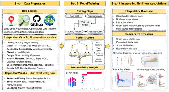
Figure 1.
Research framework.
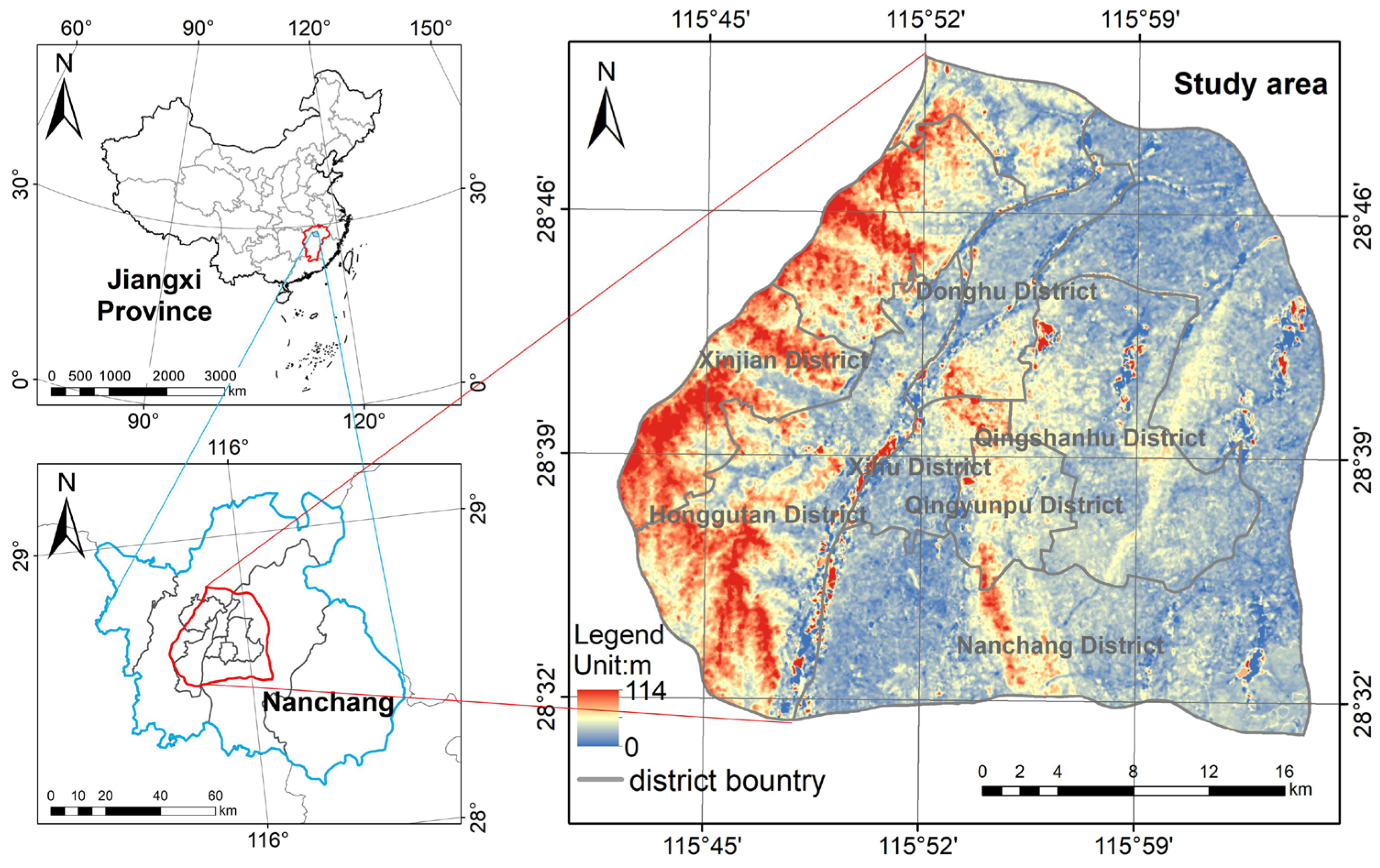
This study focused on Nanchang City, which is defined by the Third Ring Road as shown in Figure 2. As the capital of Jiangxi Province, Nanchang is in central China along the Yangtze River, with an urban population of 3.11 million and an area of 270.8 square kilometers as of 2023. Existing research on urban vitality mechanisms predominantly centers on large cities, leading to a limited understanding of vitality formation in less-developed medium-sized cities. The moderate scale within Nanchang’s Third Ring Road made it an ideal site for this investigation. In previous studies, hexagonal hierarchical geospatial indexing systems with radii of 0.1, 0.15, 0.2, and 0.25 km provided by Uber Technologies were used as the smallest study units [46,47,48]. Considering that the area within the Third Ring Road of Nanchang is relatively small, and the focus of this study was on street-level vitality, we utilized a hexagonal hierarchical geospatial indexing system with a side length of 0.1 km as the study unit, encompassing 11,943 hexagonal units. Based on these units, the average values of various geographic indicators covered by each hexagon were obtained and used as the values for that unit. Compared with traditional point and line data, the hexagonal shape better accounted for spatial heterogeneity and enhanced the coverage of streetscape data.
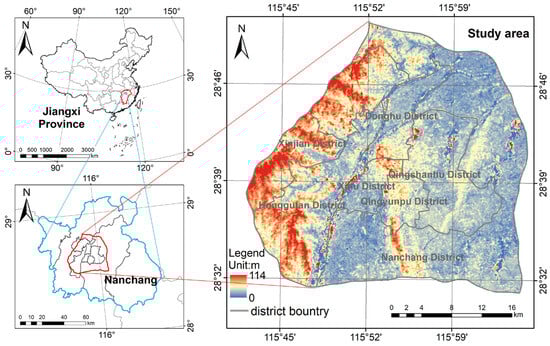
Figure 2.
Research area.
3.1. Datasets and Variables
3.1.1. Dependent Variable: Urban Street Vitality Index
The collection and processing of urban street vitality data involved several steps: (1) street view images were sourced from the Baidu Map open platform1; (2) spatiotemporal travel data were obtained from the Baidu Wise Eyes big data platform2; (3) nighttime light data for 2022 came from VIIRS3; and (4) point of interest (POI) data were accessed through the Baidu Map open platform4.
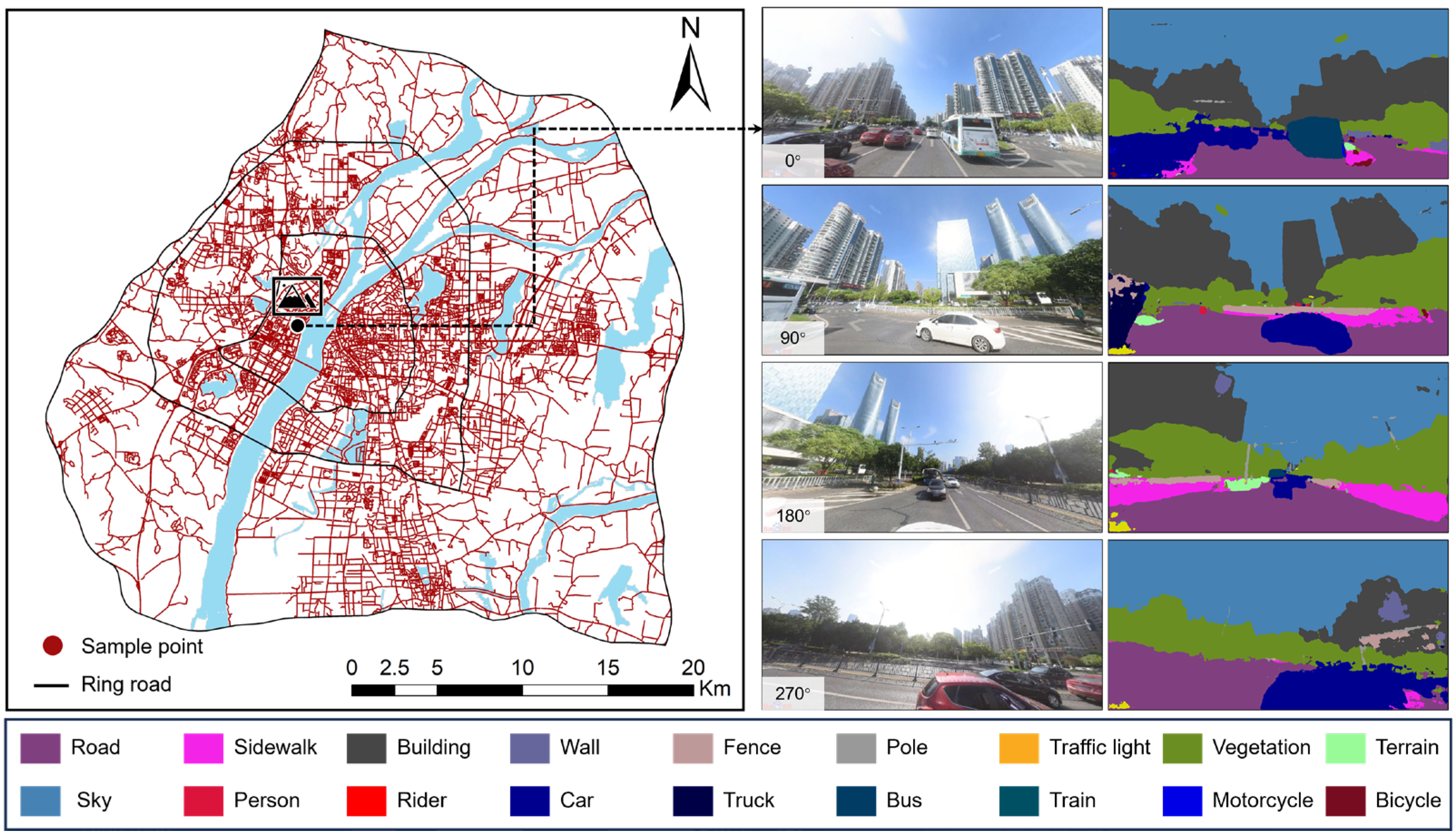
Urban street vitality was measured across three dimensions: perceptual vitality, social vitality, and economic vitality. (1) For perceptual vitality using the Baidu Map API, sample points were generated every 50 m, resulting in 37,924 points, with images captured from four directions between 2018 and 2022. These images were scored using a deep learning model trained on the Place Pulse 2.0 dataset [49]. (2) Regarding social vitality, this dimension captures population movement and nighttime activity through spatiotemporal travel data and nighttime light indices. Travel data were categorized into weekdays and weekends across three time periods: from 7:00 a.m. to 12:00 p.m., 1:00–6:00 p.m., and 7:00–11:00 p.m., while the nighttime light index was based on annual averages. (3) For economic vitality, POI richness indicates consumer activity, and the kernel density estimates for five POI categories (commercial services, residential, cultural and recreational, educational, and medical) reflect economic vitality.
To integrate the multidimensional indicators of urban street vitality into a composite index, we designed and implemented a refined two-stage principal component analysis (PCA) framework. In the first stage, PCA was applied separately to the dimensions of perceptual, social, and economic vitality, extracting the first two principal components from each to construct dimension-specific scores. In the second stage, these scores were further integrated through another PCA, ultimately yielding a comprehensive vitality index.
The PCA method applies an orthogonal transformation to convert potentially correlated variables into linearly independent principal components. Through this dimensionality reduction process, we distilled eight indicators across three dimensions into a single principal component. This transformation maximizes retention of the core information from the original data while effectively eliminating data redundancy and multicollinearity. The resulting index not only captures the latent structure of the data but also comprehensively reflects the multidimensional characteristics of urban vitality.
3.1.2. Independent Variables: Multi-Source Urban Data
The collection and processing of multi-source data included (1) elevation and slope data from the ASTER GDEM 30 m resolution digital elevation dataset5; (2) NDVI data for 2022 from the National Scientific Resources Sharing Service Platform6; (3) area data for parks, green spaces, and water bodies from Baidu Maps; (4) housing price data for 2022 from Lianjia7; (5) population density data for 2019 from WorldPop8; (6) GDP density data for 2019 from the Resource and Environmental Science Data Platform9; (7) building height and contour data from the Geographic Remote Sensing Ecological Network Platform10; (8) road network data from OpenStreetMap (OSM)11; (9) visual factors extracted using a DeepLab V3+ model trained on the Cityscape dataset, including metrics like the green view index and openness as shown in Figure 312; and (10) land use type data for 2020 from GlobeLand 3013.
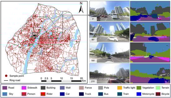
Figure 3.
Example of semantic segmentation of street view images.
This study categorized the vitality indicator variables into three main groups: (1) natural elements (elevation, slope, NDVI, and Euclidean distance to parks and water bodies); (2) sociodemographic and economic factors (population density, GDP density, and housing prices, where housing prices were processed into raster data using the inverse distance weighted method of spatial interpolation); and (3) built environment. This category reflects the 5D indicators of the built environment, selecting 5 secondary variables and 14 tertiary variables. Secondary variables included building characteristics, transport capacity, street accessibility, land use mix, and visual indicators, corresponding to the five dimensions of the built environment 5D. Density encompassed building height and density. Distance to transit was represented by the density of public transport stations and road networks. Destination accessibility was assessed through pedestrian and vehicular access, utilizing the NQPDA metrics of spatial syntax sDNA with analysis radii of 1200 and 9500. Diversity was represented by the Shannon Diversity Index, with higher SHDI values indicating richer and more fragmented land use. Design was captured through visual factors, including the green view index (GVI), sky openness index (SOI), visual enclosure index (VEI), visual walkability index (VWI), and visual motorization index (VMI). The GVI, SOI, and VEI reflect the visual landscape, while the VWI and VMI pertain to pedestrian and vehicular perceptions, respectively. The descriptions of the independent variable data are shown in Table 1.

Table 1.
Descriptions of independent and dependent variables.
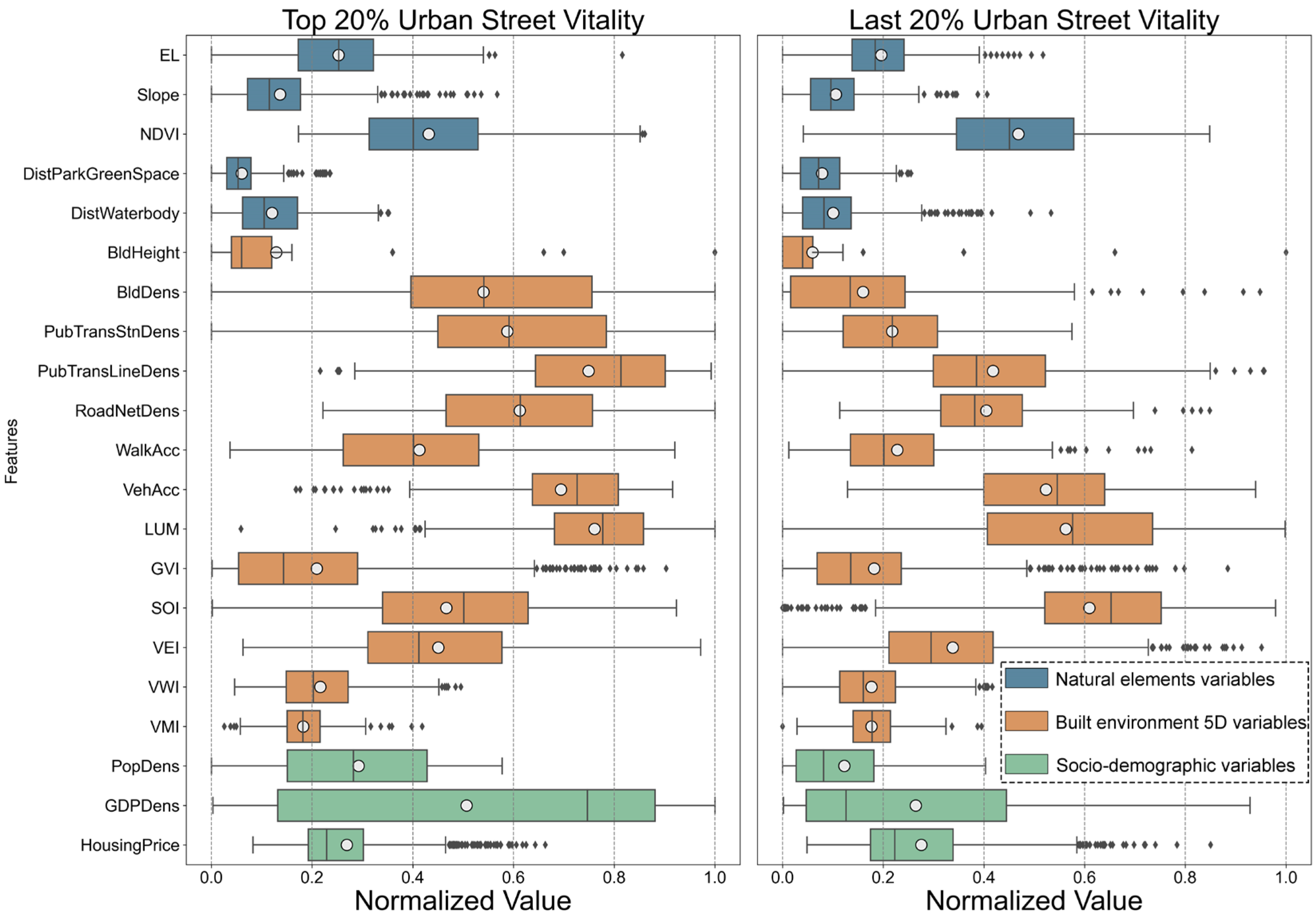
Figure 4 illustrates the multi-source data indicators and average difference ratios for the top 20% and bottom 20% of cities ranked by urban street vitality scores. It can be observed that most factors showed a positive correlation or no significant difference with vitality, while the SOI and GVI were negatively correlated with vitality.
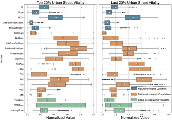
Figure 4.
Differences in indicators of urban multi-source data (top 20% and bottom 20%).
3.2. Modeling Approaches
3.2.1. XGBoost Model
XGBoost is an improvement on the gradient boosting algorithm which supports parallel computing and is suitable for handling large-scale data with its excellent efficiency and high prediction accuracy. The loss function is defined as follows:
where is the number of training samples, is the loss of a single sample, assuming it is a convex function, is the model’s predicted value for the training sample, and is the true label value of the training sample.
The modeling process in this study was carried out using the XGBoost and Scikit-learn packages (Python 3.7). First, the data were randomly divided into a training set (80%) and a test set (20%). This study applied MSE as a loss function to check the accuracy of the XGBoost model, while grid search and 5 fold cross-validation techniques were applied to obtain the optimal parameters and reduce the risk of model overfitting.
3.2.2. SHAP Model
Utilizing interpretable machine learning, SHAP explains the global and local predictions of a model and facilitates the elaboration of nonlinear effects. The Shapley value is defined as follows:
where: is the contribution of the th feature to the predicted value of instance , is the subset of all features except , is the number of features in subset S, is the total number of features, is the value predicted by the model given the feature subset , and is the value predicted by the model given the feature subset plus the feature.
Then, a single prediction is interpreted as follows:
In the formula, represents the predicted street vitality value, indicates whether the corresponding feature exists in the decision path, is the number of input features, is a constant, and is the SHAP value of feature .
This study uses Shapley interaction values to determine the interaction synergy effect between variables on urban vitality. Interaction synergy refers to the effect that occurs when two or more factors or variables interact with each other such that their combined effect is greater or less than the sum of the factors when they act individually:
When , we have
where is the Shapley interaction value, reflecting the interactive effect of variables and on a single prediction, is the number of variables, is the input variable set, is the possible variable coalitions, and is the predicted input variable value.
This study used the TreeExplainer interpreter of the SHAP package (Python 3.7) to interpret the XGBoost model. Using TreeExplainer, the global relative importance and local nonlinear interpretations of variables from multiple data sources could be obtained, along with interaction synergies and clustering of urban street vibrancy based on the similarity of local effects, revealing patterns in model behavior.
4. Results
4.1. Model Performance Comparison
In this study, we implemented a two-stage PCA framework to construct a composite measure of urban street vitality. In the first stage, we performed dimensionality reduction separately for each of the three vitality dimensions, extracting the first two principal components from each to obtain corresponding vitality scores. As shown in Table 2, the cumulative variance explained by the first two components for each dimension reached significant levels—86.4% for perceptual vitality, 96.0% for social vitality, and 94.2% for economic vitality—indicating that this reduction strategy effectively preserved the core information of the original indicators. In the second stage, we applied PCA again to integrate the scores from these three dimensions, ultimately constructing a single comprehensive index representing the overall urban street vitality. This approach maintained the integrity of the multidimensional characteristics of street vitality while ensuring analytical simplicity.
Table 2.
Description of cumulative explained variance ratio.
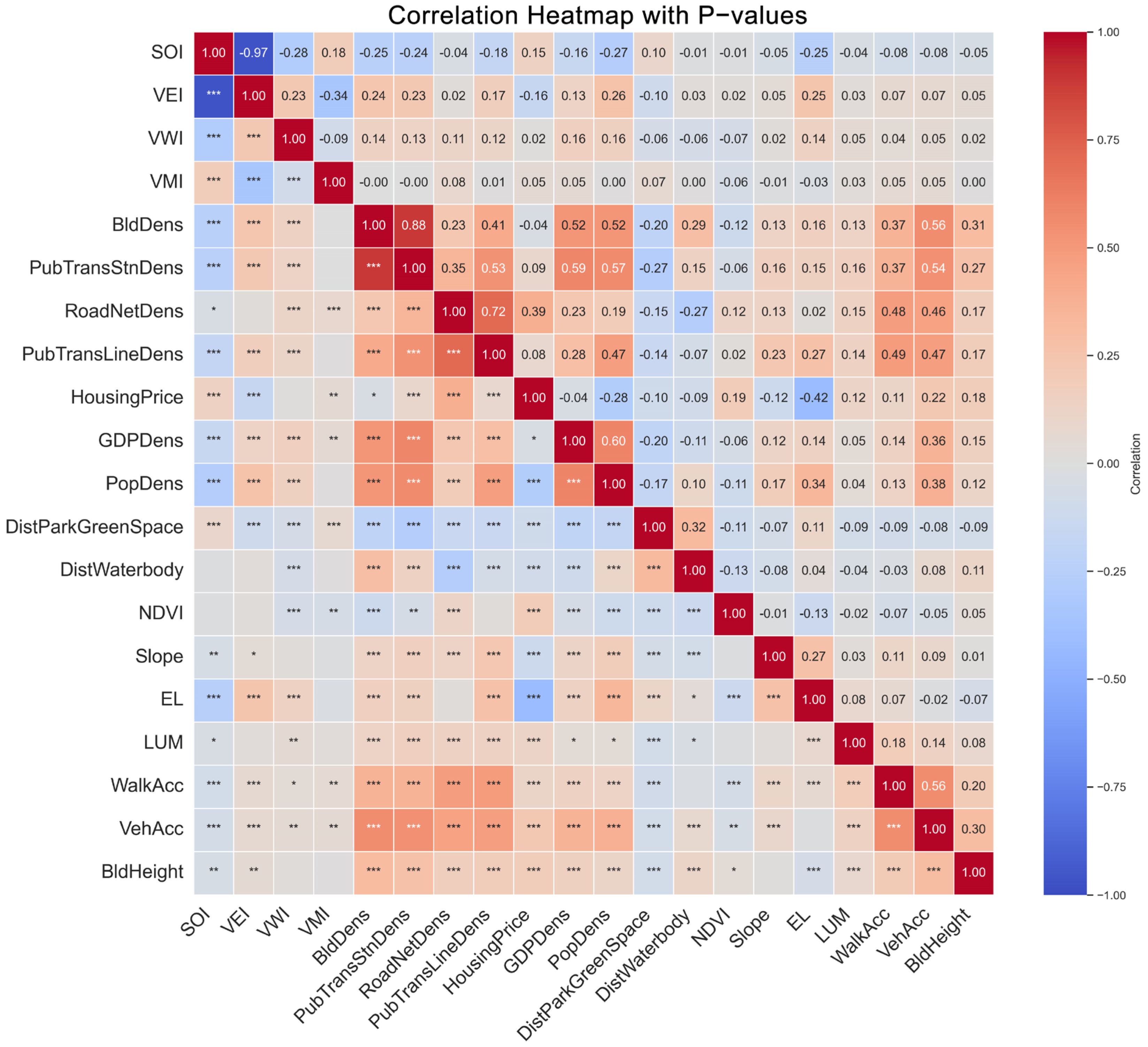
Prior to constructing the XGBoost model, Pearson correlation analysis (Figure 5) and variance inflation factor (VIF) checks were conducted to eliminate variables with a VIF >10 and excessively high correlation coefficients. The analysis indicated that, except for the SOI and NDVI, all other indicators positively correlated with urban street vitality. Negative correlations were primarily found in areas with low building densities and high green coverage in peripheral urban zones. Transportation-related variables, specifically PubTranLineDens and PubTranStnDens, exhibited the highest positive correlations, suggesting that convenient public transport enhances vitality.
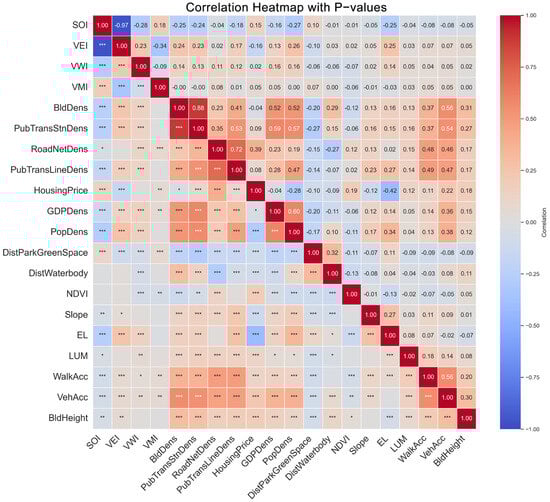
Figure 5.
Pearson correlation analysis of urban multi-source data. * p < 0.05. ** p < 0.01. *** p < 0.001.
After addressing multicollinearity by removing problematic indicators, the XGBoost model was compared with nine other models, including OLS, RF, and SVR, using MSE, MAE, and R² as evaluation metrics. Hyperparameters were optimized through grid search and k-fold cross-validation to mitigate overfitting.
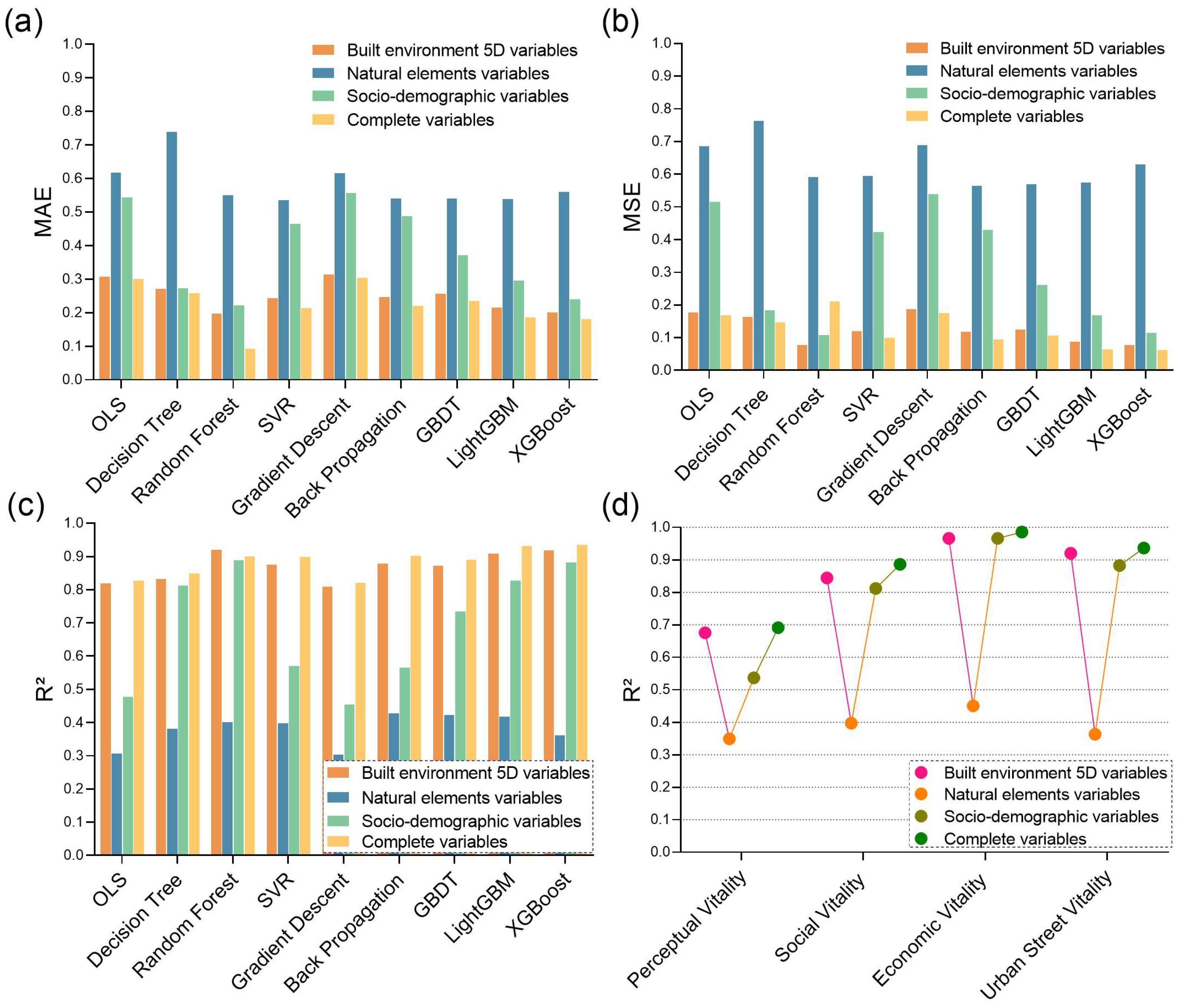
Figure 6a–c demonstrates that the datasets with urban multi-source data variables outperformed those with single variables across all models. At the algorithmic level, XGBoost achieved superior performance, with R², MSE, and MAE values of 0.936, 0.182, and 0.063, respectively. Figure 6d shows the predictive performance of urban street vitality and its three subdimensions (economic vitality, social vitality, and perceptual vitality) when using the XGBoost model on various dataset combinations. The datasets containing urban multi-source data variables exhibited the highest fitting performance in each dimension, with R² values of 0.691, 0.886, 0.985, and 0.936, indicating the enhanced explanatory power of urban multi-source data across different dimensions of urban street vitality.
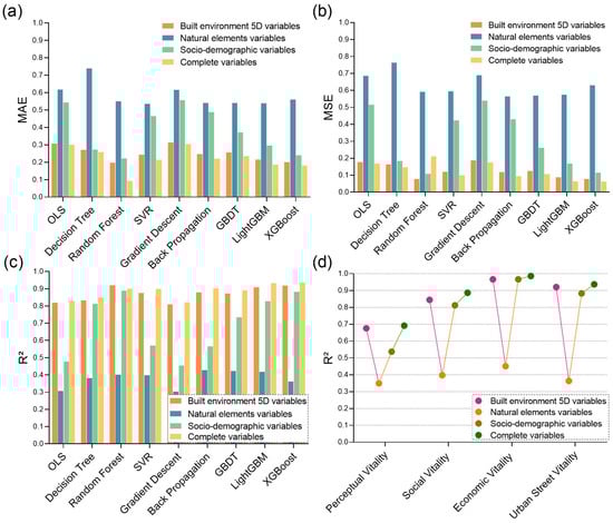
Figure 6.
(a–c) Performance comparison of different models under different dataset combinations. (d) Model performance indicators of different dimensions of urban street vitality.
4.2. Nonlinear Explanations
4.2.1. Relative Importance of Urban Multi-Source Data Across Different Dimensions of Urban Street Vitality
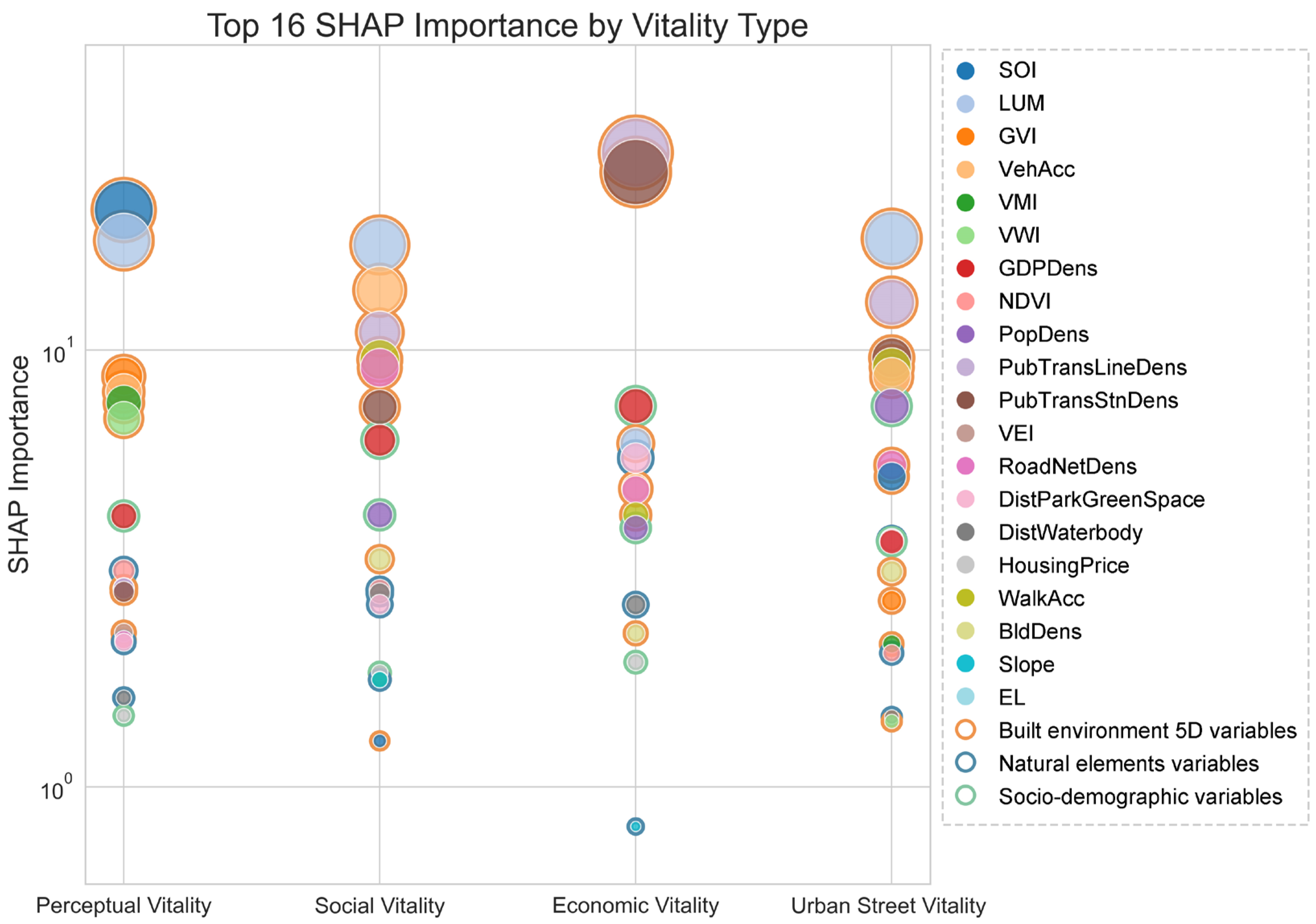
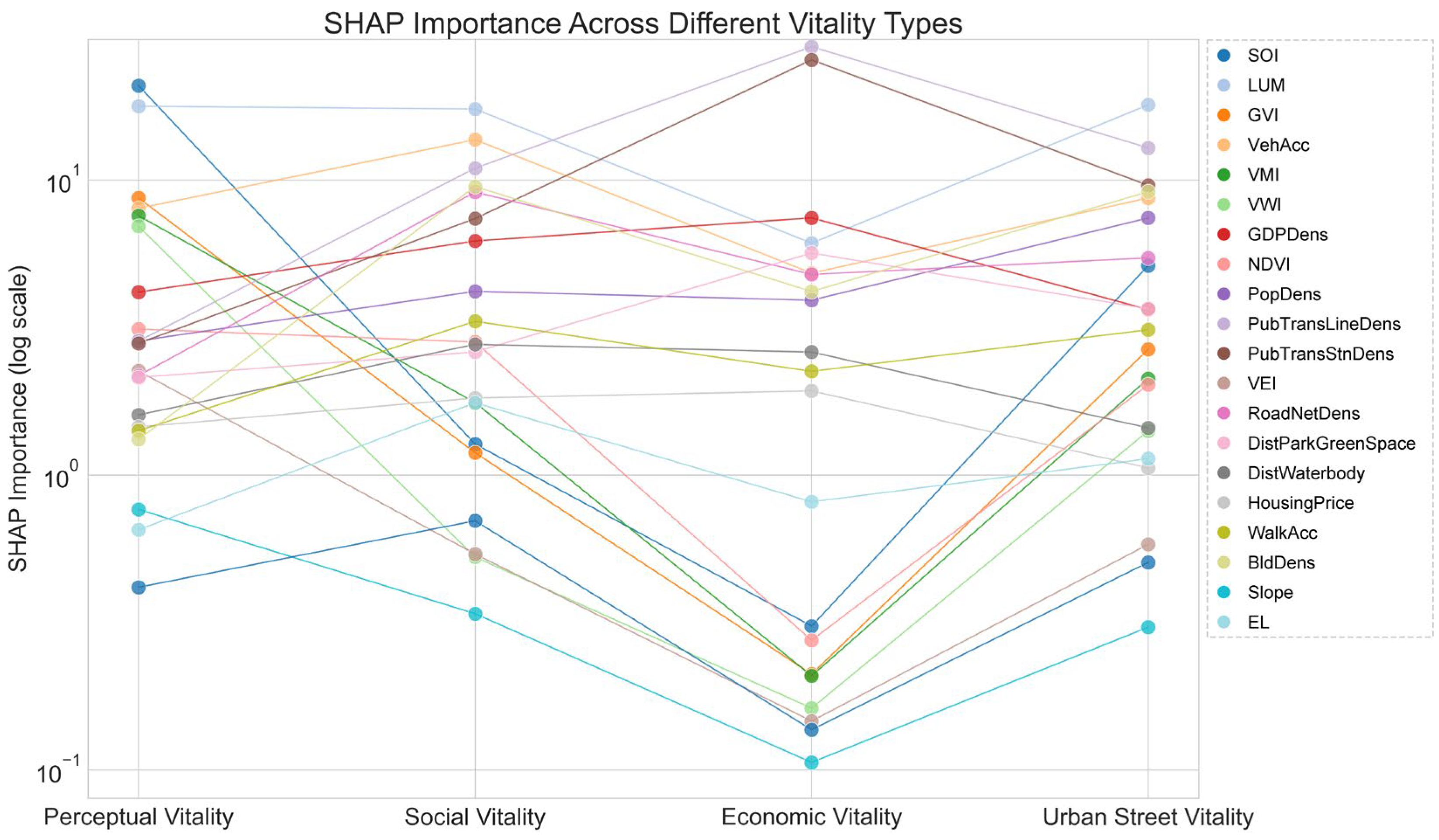
Figure 7 visually presents the global feature importance of driving factors across different dimensions of urban street vitality, with variables arranged in descending order of global importance, highlighting the top 16 indicators for each vitality dimension. Figure 8 shows the changes in the global feature importance of various variables across different dimensions of urban street vitality.
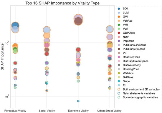
Figure 7.
Global feature importance diagram of SHAP model.
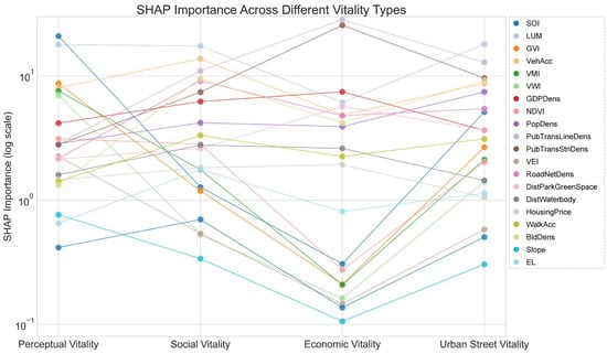
Figure 8.
Changes in the global feature importance of each variable in different dimensions of urban street vitality.
As shown in Figure 7, from the perspective of vitality dimensions, LUM, PubTransStnDens, PubTransLineDens, and VehAcc consistently made significant contributions across all four vitality dimensions. In the primary urban street vitality dimension, the five indicators contributing the most were LUM, PopDens, PubTransStnDens, PubTransLineDens, BldDens, and VehAcc. Notably, BldDens had lower importance in other vitality dimensions. Overall, most driving factors showed stable feature importance across the four vitality dimensions, but in the perceptual vitality dimension, the SOI’s importance significantly rose to first place. In the economic vitality dimension, both PubTransStnDens and PubTransLineDens also saw a significant increase in importance, while the importance of LUM and the VMI declined.
In terms of driving factor types, indicators related to diversity, population, and transportation capacity significantly influenced various dimensions of urban street vitality. Among natural elements, the influence of EL and Slope was minor, except for DistPark&GreenSpace. In the sociodemographic and economic dimensions, PopDens and GDPDens ranked 2nd and 10th, respectively, as significant factors affecting urban street vitality, related to the population and economic agglomeration effects in urban centers.
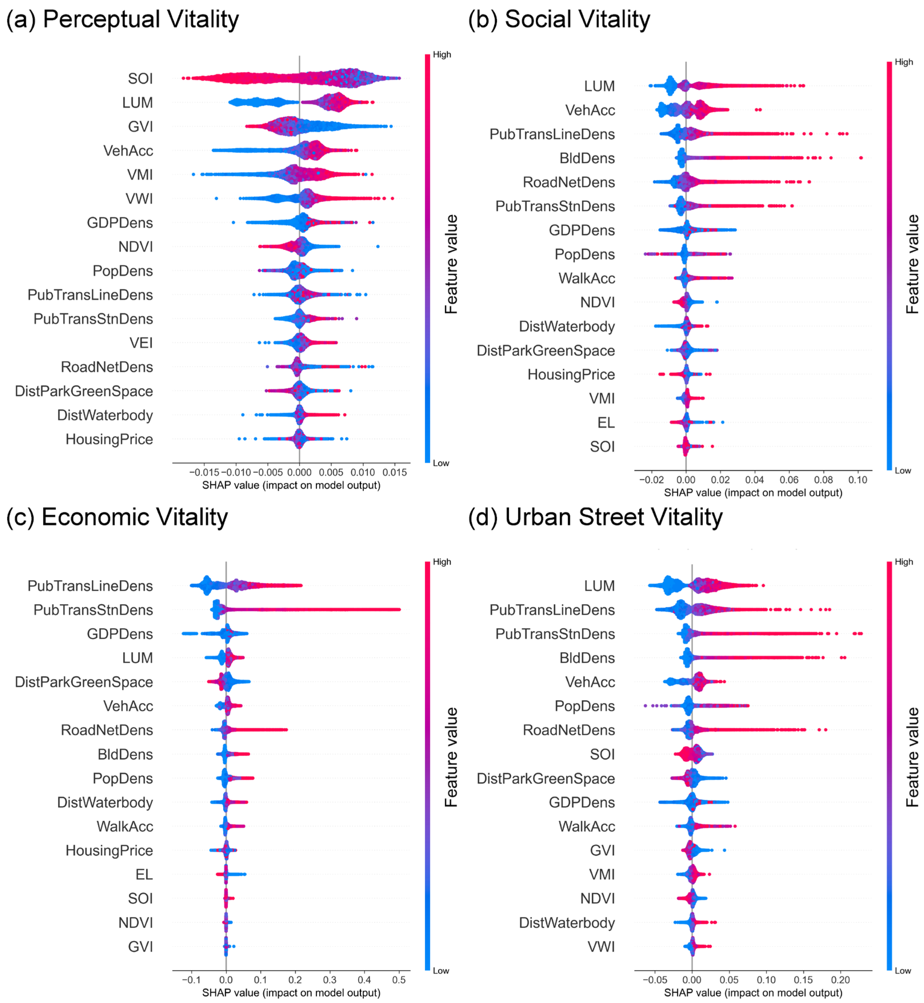
Figure 9 presents local explanation plots for the driving factors across different dimensions of urban street vitality, where red-to-blue points represent feature values from high to low, and the SHAP values on the x axis indicate positive and negative impacts on urban street vitality. As shown in Figure 9, similar to the descriptive analysis results, the majority of the driving factors exhibited positive correlations, while the NDVI, SOI, and GVI elements showed significant negative correlations. These three elements reflect natural and sky conditions, likely related to the high density of buildings within urban built-up areas and a scarcity of natural elements.
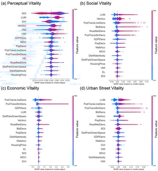
Figure 9.
Local relative importance diagram of SHAP model.
4.2.2. Nonlinear Associations Between Urban Multi-Source Data and Urban Street Vitality
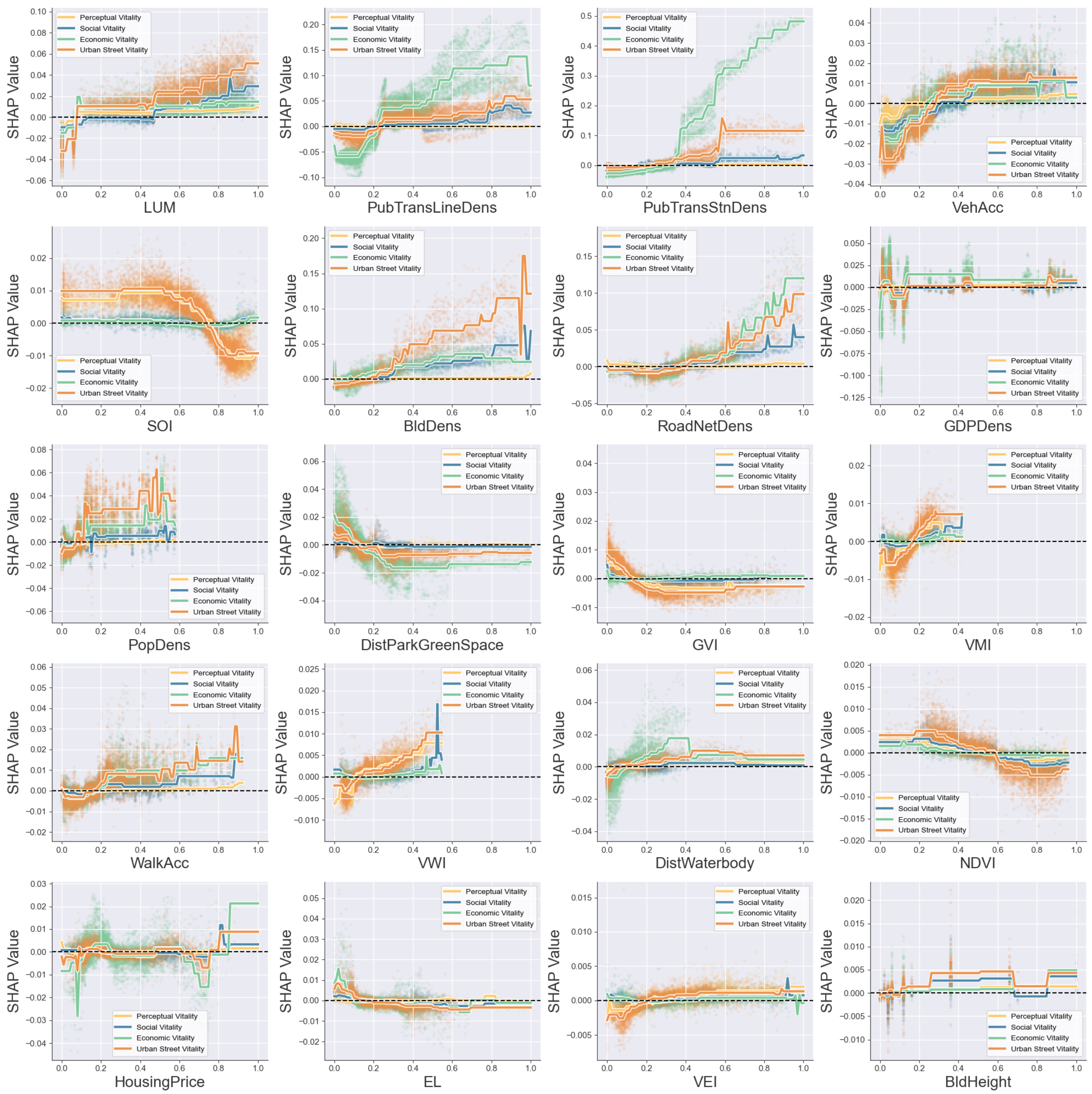
This study examined the nonlinear and threshold effects of individual independent variables on the dependent variable using local dependence plots, where the x-axis represents the normalized variable values and the y axis shows the SHAP values. By integrating the local dependence plots for the four vitality dimensions, the feature importance was averaged and ranked across these dimensions (Figure 10).
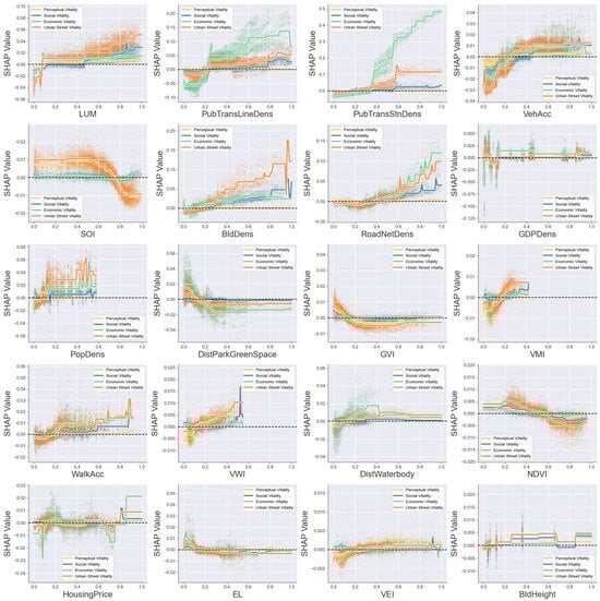
Figure 10.
SHAP local dependence diagram of urban multi-source data on different dimensions of street vitality.
As shown in Figure 10, most independent variables exhibited consistent curve trends across different vitality dimensions, but there were significant differences in the curves of certain variables. In the built environment dimension, the curve trend of LUM was similar; the SHAP values for LUM in the lowest 20% were less than zero, while those in the highest 80% correlated positively with street vitality. This indicates that a higher degree of land mixing promotes more social and economic activities, thereby enhancing street vitality. PubTransStnDens and PubTransLineDens generally exhibited positive correlations, with SHAP values predominantly above zero. Particularly in the economic vitality curve, their curve slope was maximal, indicating that convenient public transport enhances economic vitality by attracting foot traffic. The BldDens variable remained stable in the perceptual vitality dimension but showed a significant positive effect in the urban street vitality dimension, with SHAP values consistently above zero, indicating that while dense buildings do not enhance sensory experience, they can improve the overall street vitality. The SOI and GVI had negative impacts on street vitality, particularly in the perceptual vitality and urban street vitality dimensions. The SOI followed an inverted U-shaped curve, with SHAP values dropping below zero near the turning point, suggesting that moderate openness to the sky enhances street vitality, while excessive openness reduces it. GVI data indicate that limited greenery positively affects street vitality, while high-vitality areas typically feature less street greenery.
In the natural elements dimension, the NDVI and DistWaterbody had a negligible impact on the vitality, while smaller values of DistPark&GreenSpace corresponded to higher vitality values, which was particularly evident in the economic vitality curve, suggesting that commercial locations favor proximity to parks and green spaces. In the population and economic indicator dimension, PopDens generally showed an upward trend, but the lowest 10% of the rankings had SHAP values below zero. The SHAP values began to rise from negative values, peaking at higher PopDens ranges before declining again, indicating that both extremely low and extremely high population densities negatively affect street vitality, while moderate increases in population density can enhance it.
Overall, the curved trends across different dimensions of urban street vitality indicate that urban street vitality showed the steepest slopes for most variables, while perceptual vitality had the shallowest slopes. This suggests that urban street vitality is more sensitive to variations in urban multi-source data variables, while perceptual vitality is primarily influenced by design-related variables, as these reflect the proportion of visual elements. Furthermore, the economic vitality dimension was more sensitive to the variables of PubTransLineDens and PubTransStnDens, showing lesser influence from changes in other variables.
4.3. Spatial Heterogeneity and Distribution of Urban Street Vitality
Figure 11a–d illustrates the spatial distribution of urban street vitality and its three dimensions, along with the corresponding Moran’s I index scores. Higher-vitality areas were primarily located within the inner ring and urban built-up zones, with a gradual decline toward the outskirts, while vitality indices were lower in the third ring. Moran’s I index indicated a positive spatial correlation among the vitality areas, except for the perceptual vitality dimension, which had an index of 0.56; the indices for other dimensions were notably higher. The spatial distribution differences in perceptual vitality suggest that the vitality calculated through traditional indicators differed from that perceived visually, highlighting the importance of incorporating the perceptual dimension into urban street vitality analysis.
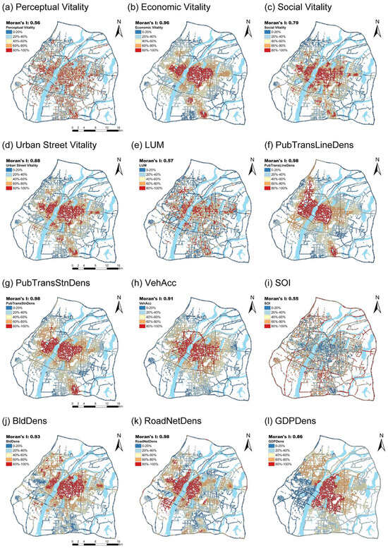
Figure 11.
Spatial distribution and Moran’s I index values of different dimensions of urban street vitality.
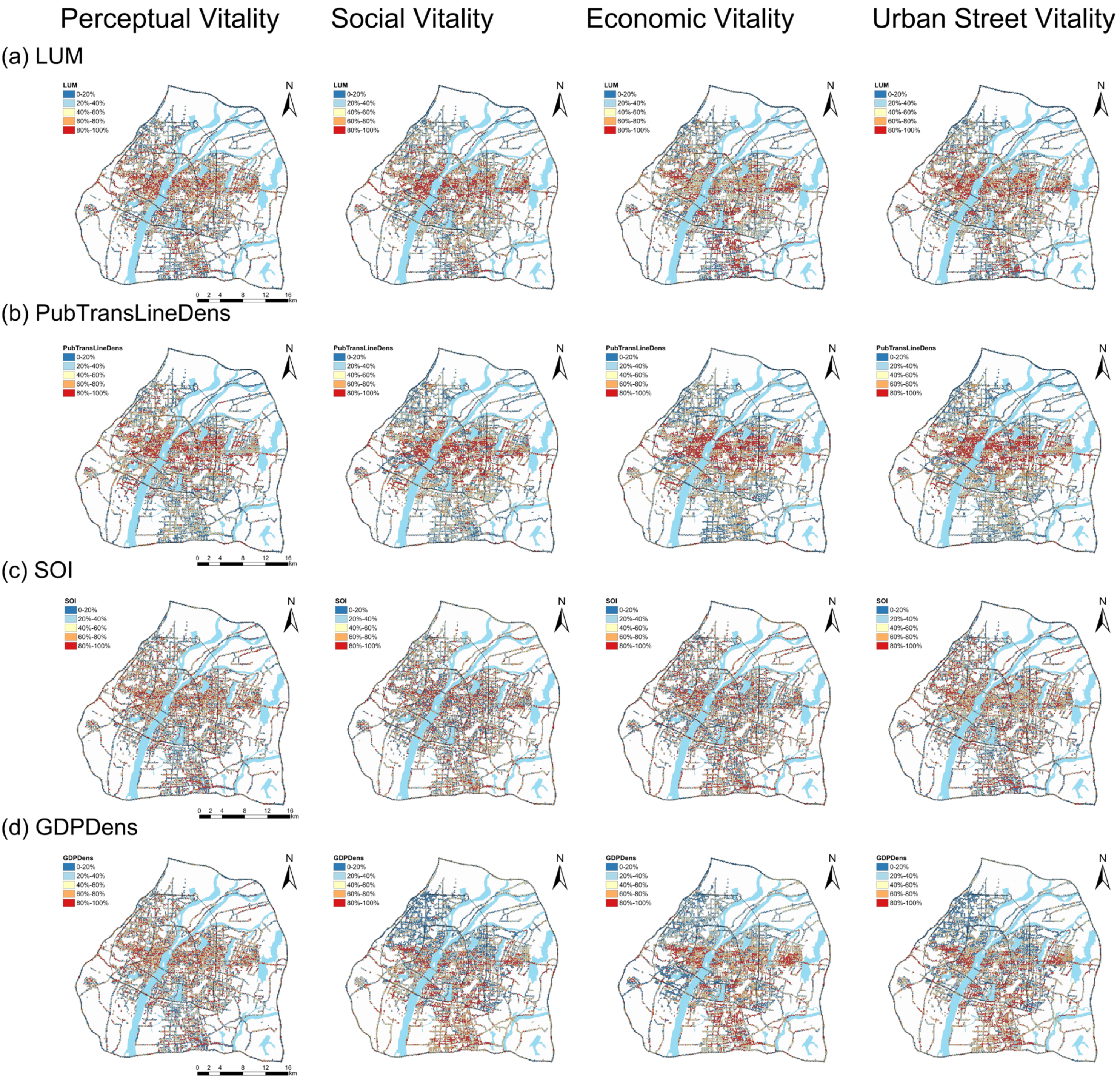
This study also presents the spatial distribution of SHAP values for the major driving factors across different vitality dimensions (Figure 12). Most driving factors exhibited similar spatial distributions and effects across the four dimensions, with LUM, PubTransLineDens, and the SOI having a positive influence on research units within the inner ring. GDPDens demonstrated a positive effect in other vitality dimensions, primarily concentrated in areas with high total GDP values, while in the perceptual vitality dimension, it was located within the inner ring. This indicates that a developed economy promotes renovation of the appearance of aging buildings within the inner ring [50].
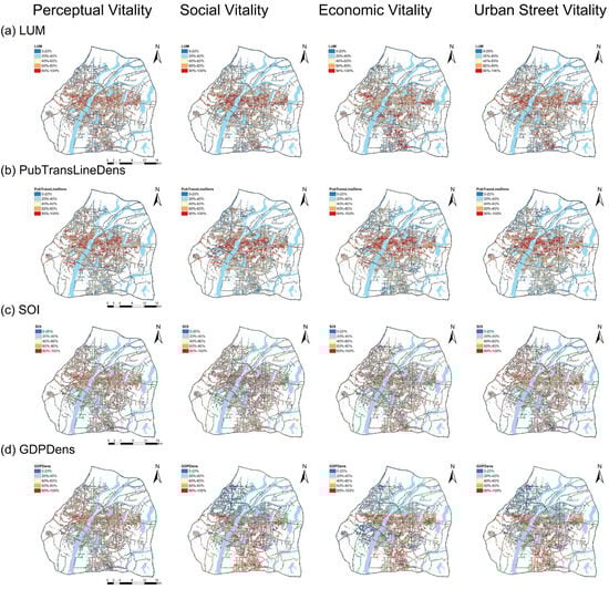
Figure 12.
Distribution of SHAP values for major driving factors across different dimensions of urban street vitality.
4.4. Interactive Effects of Key Variables in Urban Multi-Source Data
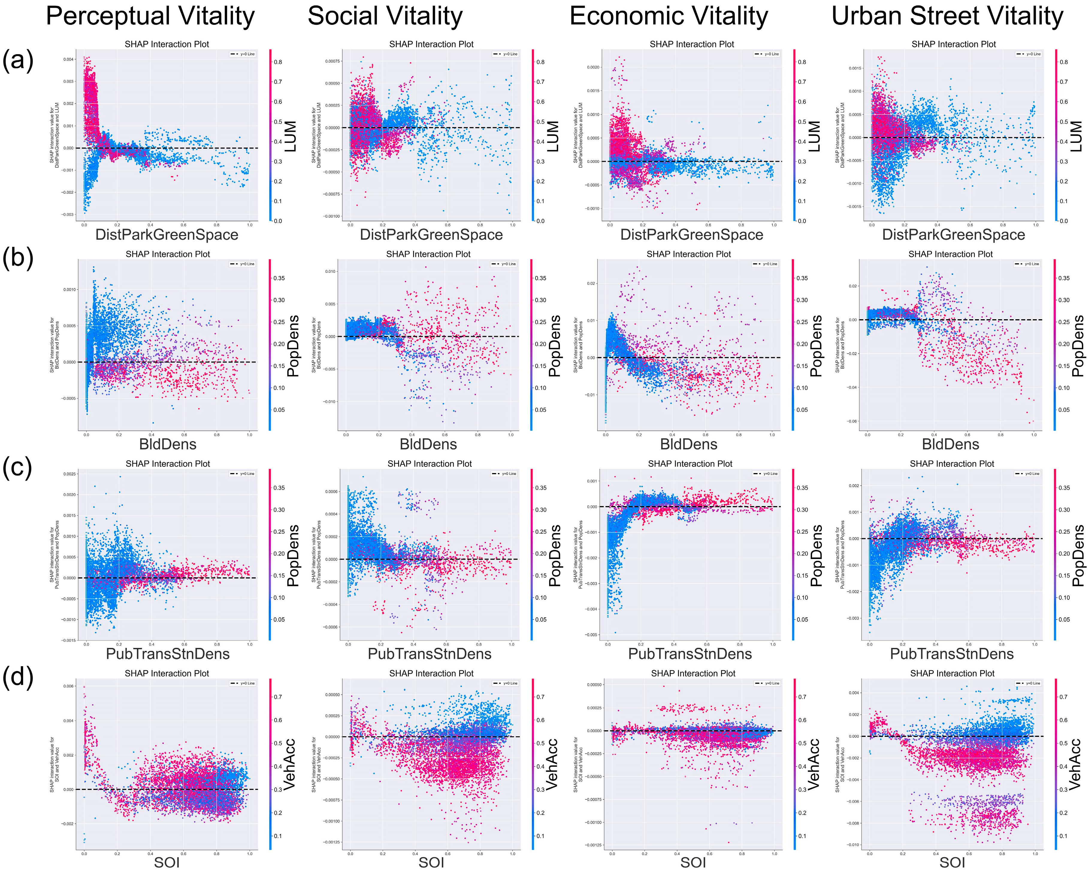
Figure 13 illustrates the interactive effects between the most significant variables in urban multi-source data across different dimensions. The x axis represents one independent variable, with different colors indicating the magnitude of another independent variable (points closer to red indicate higher values), while the y axis represents the interaction value between the two. The position where the SHAP interaction value equals zero serves as a reference line. Samples above this line indicate a positive correlation between the indicator and the dependent variable.
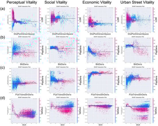
Figure 13.
Interaction effects between major variables in different dimensions of vitality; (a) DistParkGreenSpace vs. LUM; (b) BldDens vs. PopDens; (c) PubTransStnDens vs. PopDens; (d) SOI vs. VehAcc.
The interaction effects among variables were relatively similar across different vitality dimensions. Figure 13a displays the interaction between LUM and DistParkGreenSpace across the four vitality dimensions. When in proximity to parks and green spaces and with higher land mixing, the SHAP interaction value reached its peak, indicating that these areas enhance the positive impact of land mixing on street vitality.
Conversely, in areas farther from parks and green spaces, the contribution of land mixing to street vitality diminished. Figure 13b shows that moderate population densities and building densities positively affected vitality across dimensions, whereas an excessive density had a negative impact. This suggests that increased building and population densities can enhance commercial activity and social interaction, thus boosting street vitality, while an excessively high density may lead to discomfort, which was particularly evident in the perceptual vitality dimension. Figure 13c illustrates the interaction between PubTransStnDens and PopDens. In all four vitality dimensions, areas with high bus stop densities and high population densities had a positive effect on vitality. However, in the contexts of perceptual vitality and social vitality relative to economic vitality and urban street vitality, differences arose in the interaction values for low bus stop densities and population densities. In the latter two cases, low bus stop densities and population densities negatively affected vitality, while the former two exhibited a coexistence of positive and negative effects. This indicates that areas with well-developed public transportation facilities can facilitate substantial population movement, significantly enhancing street vitality. Conversely, areas with low levels of both may be in underdeveloped or ecologically favorable regions on the urban periphery, thus reflecting mixed effects on perceptual vitality. Figure 13d indicates that areas with high vehicle accessibility and a low SOI positively impacted vitality, whereas those with both high vehicle accessibility and a high SOI negatively affected vitality. Areas with higher vehicle accessibility are typically located within cities, being characterized by a greater building density and lower SOI, suggesting that increased openness to the sky has a limited effect on enhancing street vitality in well-connected areas.
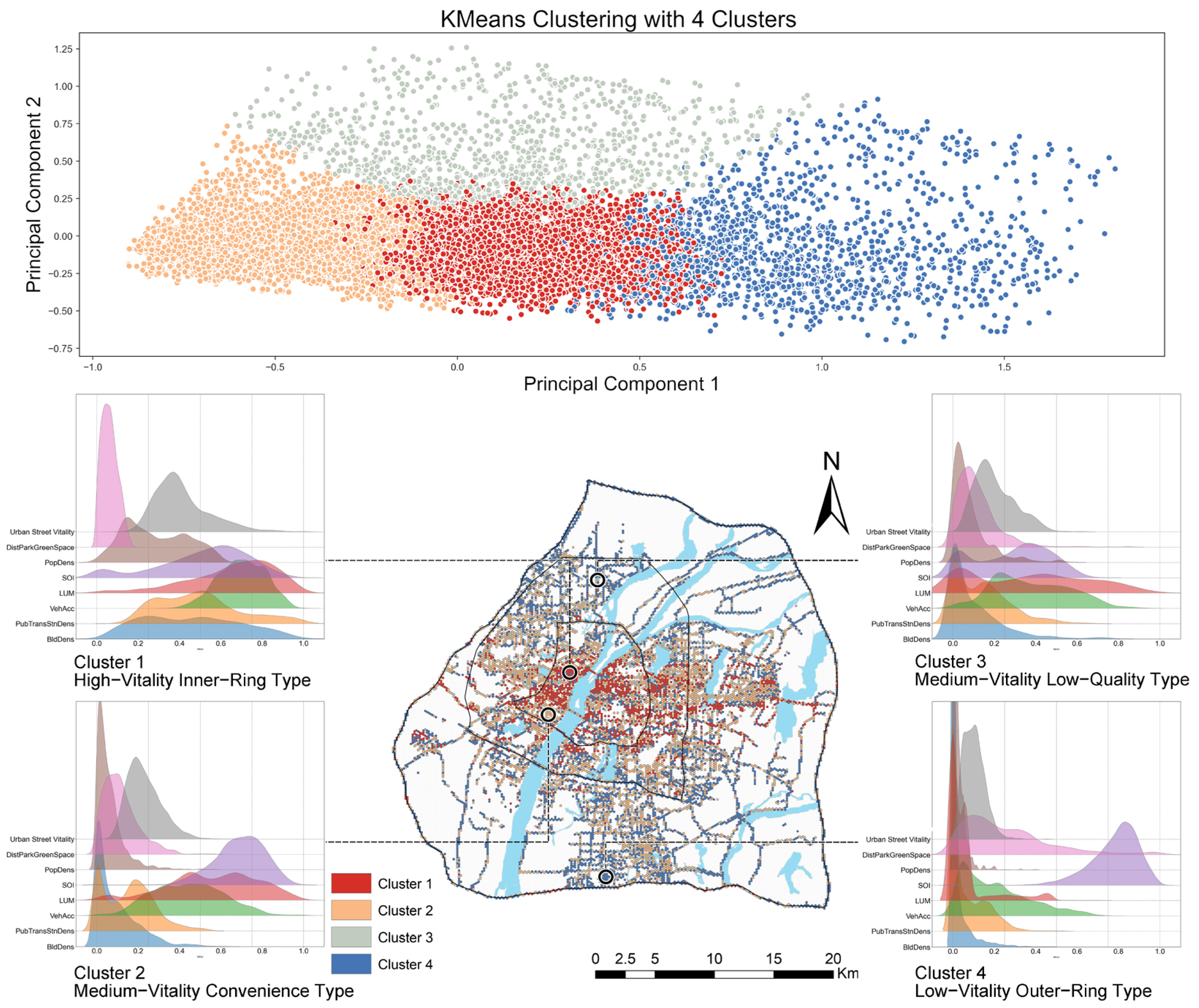
Analyzing the similar local effect patterns of urban multi-source data on street vitality can provide valuable insights for urban planning enhancement. Specifically, this study employed K-means clustering to analyze the similarities in local effects among streets, generating meaningful clusters. Figure 14 illustrates four types of street vitality: the high-vitality inner ring (13.8%), moderate vitality convenient type (37.7%), moderate-vitality low-quality type (9.4%), and low-vitality outer ring (38.9%). The clusters exhibit spatial aggregation and reveal key influencing factors for each street type through visualizing multi-source data.
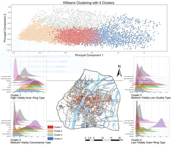
Figure 14.
Distribution of urban streets for different vitality types and representative cases.
High-vitality inner ring streets are in the urban core and are characterized by high population densities, mixed land use, well-developed public transportation, and proximity to natural spaces, reflecting a concentration of economic and social vitality. The moderate-vitality convenient type is found in old urban areas and along major transport routes, exhibiting high sky openness and balanced building densities, which enhance residents’ quality of life. The moderate-vitality low-quality type features low building densities and public transportation densities, lacking vitality and primarily being concentrated in low-quality areas of city centers. Low-vitality outer ring streets are predominantly located on the urban periphery and characterized by high sky openness but minimal values for other variables, indicating a lack of vitality in these areas. This suggests that future urban planning should balance infrastructure and service distribution to promote sustainable development in peripheral areas.
5. Discussion
5.1. Interpretable Machine Learning Framework
This study revealed the distinct effects of urban multi-source data variables on the four dimensions of street vitality by integrating urban multi-source data and interpretable machine learning models, offering new perspectives for urban planning. This indicates that, in addition to traditional built environment factors, urban planners should also consider natural landscapes and socioeconomic factors to create more vibrant and livable urban spaces [14]. The introduction of nonlinear and interpretable machine learning models transcends the limitations of linear assumptions, accounting for interactions among variables and addressing the black box problem of models, thereby providing data-driven insights for urban planning and design.
5.2. Comprehensive Explanation of Urban Street Vitality
Most indicators across the dimensions of urban street vitality were positively correlated with street vitality. Although some indicators, such as DisParkGreenSpace and the SOI, showed minimal variation in descriptive analysis, they contributed significantly to the SHAP model, revealing a nonlinear relationship and threshold effects of urban multi-source data on street vitality. There was a correlation between the spatial distribution of urban street vitality and its three subdimensions (perceptual, economic, and social vitality), with high-vitality areas concentrated in the urban core. In contrast, the lower spatial correlation of perceptual vitality reflects the diversity of human subjective perception [51].
Overall, the built environment variables had the most significant impact on vitality followed by socioeconomic population variables, while natural elements had the least effect. This study found that the positive effect of land use mixing was strongest as increasing the degree of land use mixing can enhance population flow and interaction, and a higher degree of mixing also implies a greater variety of facilities impacting daily life [52]. Unlike previous studies, this research suggests that the impacts of slope and elevation on street vitality are limited. This is because modern cities can mitigate the effects of these factors through modification of the natural environment. Meanwhile, previous studies considered the impacts of building density and height to be similar [25]. However, this study found that the effect of building density is greater than that of building height, which was particularly evident in the urban street vitality dimension.
PubTransStnDens, PubTransLineDens, and the SOI were the variables with significant fluctuations in importance. This may indicate that at the economic vitality level, convenient urban public transportation provides a favorable commuting environment for workers, whose economic growth and consumption can enhance vitality in the economic dimension [18]. At the perceptual vitality level, the openness of the sky can create feelings of alienation or crowding for individuals, thereby influencing their movement within such areas. The results from the local dependence plots for each dimension indicate that many built environment variables exhibited diminishing positive effects beyond a certain threshold, while the GVI and SOI demonstrated negative threshold effects. Similarly, natural element variables (such as the NDVI) may shift from positive to negative impacts after reaching a threshold, highlighting the importance of focusing on threshold ranges in urban planning to enhance resource allocation efficiency.
The interaction effects among multi-source data variables reveal the synergistic influences between them. The interaction plot of BldDens and PopDens indicates that areas with high population densities but low building densities negatively affect street vitality, demonstrating that excessively sparse areas struggle to attract foot traffic [53]. In densely populated areas, moderately increasing the building density is an effective strategy for enhancing street vitality, necessitating sound urban planning to avoid overcrowding and ensure high-quality public spaces. The interaction plot of the SOI and VehAcc suggests that urban planners should focus on enhancing sky openness, particularly in areas with high vehicular accessibility. By increasing green spaces, optimizing architectural designs, and planning open spaces, urban vitality can be enhanced. The interaction plot of PubTransStnDen and PopDens highlights the role of optimizing the public transportation network and enhancing station coverage in boosting vitality in densely populated areas. The interaction plot of DistPark&GreenSpace and LUM indicates that in areas close to parks and green spaces, urban planners need to carefully design land use to avoid negative effects from excessive mixing, while in areas farther from parks and green spaces, moderately increasing land use mixing can serve as a strategy to enhance street vitality [54].
5.3. Significance of This Study
By analyzing the local effect patterns of urban multi-source data, tailored planning recommendations are proposed for four street categories. For high-vitality inner ring streets in the urban core, optimizing public transportation could alleviate traffic congestion, improve travel efficiency, and boost regional vitality. Increasing green spaces and recreational areas can enhance the environment, improve quality of life, and foster social and cultural activities. Moderate-vitality convenient streets, characterized by accessible transportation, exhibit higher vitality, and enhancing connectivity, particularly through the expansion of public transport networks, can stimulate foot traffic and commercial activity. Moderate-vitality low-quality streets are typically located in areas with poor environmental quality. Urban renewal and environmental remediation can improve building quality and resident well-being. Improving infrastructure is essential for enhancing residential comfort and quality of life. Low-vitality outer ring streets are constrained by inconvenient public transportation. Expanding public transport networks, introducing commercial facilities, and providing job opportunities can stimulate economic and social vitality in these areas.
6. Conclusions
This study leveraged urban multi-source data to propose an innovative machine learning framework for analyzing and interpreting the nonlinear associations and interaction effects between urban street vitality and multi-source data variables. The XGBoost model addresses nonlinear relationships, while SHAP provides both global and local interpretations. This approach systematically examines the relationships between various dimensions of street vitality and multi-source data, highlighting the distinct characteristics of different vitality types of streets.
The findings indicate the following. (1) Urban street vitality exhibited a significant positive spatial correlation, with built environment 5D indicators primarily determining the vitality. (2) The influence strength and importance of multi-source data variables varied across different dimensions of street vitality, such as the impact of traffic station density on economic vitality, which significantly increased. (3) Built environment 5D indicators, particularly land use mix and public transport-related variables, significantly contributed to vitality. (4) Complex relationships existed among the factors influencing street vitality, producing varying effects under different thresholds and conditions. (5) Cluster analysis revealed unique land use patterns, architectural characteristics, demographic structures, and socioeconomic backgrounds for each urban vitality type.
This research provides data-driven insights for urban planners, aiding in the identification and optimization of the key factors affecting street vitality and supporting the formulation of personalized and targeted planning strategies. However, this study has the following limitations. First, we did not fully account for the temporal dynamics of urban vitality, which can be influenced by factors such as seasonality, economic cycles, and social changes. Second, variations in seasonality and lighting in street view images may affect the accuracy of the data, while the low precision of some geographic data could also impact the reliability of the results. Moreover, the lack of transfer modeling analysis across multiple underdeveloped cities limits the broader applicability of the findings.
To address these limitations, future research should incorporate time series data to analyze the dynamic trends of urban vitality and its influencing factors. Additionally, large-scale transfer learning combined with spatial autocorrelation-based nonlinear models will help develop a more comprehensive understanding of the factors influencing street vitality across different urban contexts. These improvements will enhance the depth and broader applicability of the research, providing a stronger theoretical foundation for the study of urban vitality.
Author Contributions
Conceptualization, Y.X. and J.Z.; methodology, Y.X., J.Z. and Y.L.; software, Y.X., Z.Z. and J.D.; formal analysis, Y.X., Z.Z. and J.D.; data curation, Y.X.; writing—original draft preparation, Y.X., Z.Z. and J.D.; writing—review and editing, J.Z.; supervision, Z.L. All authors have read and agreed to the published version of the manuscript.
Funding
This research was funded by the Key Research Base of Humanities and Social Sciences of Universities in Jiangxi Province (grant number JD23003) and National Social Science Fund Project: Sociological Research on Spatial Regeneration and Ethical Cultural Reconstruction of Traditional Villages (grant number 20BSH089).
Data Availability Statement
Data and materials are available from the authors upon request.
Acknowledgments
The authors thank the anonymous reviewers for their valuable comments and suggestions on this article.
Conflicts of Interest
The authors declare no conflicts of interest.
Notes
| 1 | https://lbsyun.baidu.com/, accessed on 2 August 2024. |
| 2 | https://huiyan.baidu.com/, accessed on 2 August 2024. |
| 3 | https://eogdata.mines.edu/products/vnl/, accessed on 2 August 2024. |
| 4 | See note 1 above. |
| 5 | https://www.gscloud.cn/home, accessed on 2 August 2024. |
| 6 | https://www.resdc.cn/, accessed on 2 August 2024. |
| 7 | https://bj.lianjia.com/, accessed on 4 August 2024. |
| 8 | https://www.worldpop.org/, accessed on 4 August 2024. |
| 9 | https://www.resdc.cn/, accessed on 4 August 2024. |
| 10 | http://gisrs.cn/index.html, accessed on 4 August 2024. |
| 11 | https://www.openstreetmap.org/, accessed on 5 August 2024. |
| 12 | https://www.cityscapes-dataset.com/, accessed on5 August 2024. |
| 13 | https://www.webmap.cn/, accessed on 5 August 2024. |
References
- Jacobs, J. The Death and Life of Great American Cities; Vintage: New York City, NY, USA, 1961. [Google Scholar]
- Gehl, J. Life Between Buildings: Using Public Space; Island Press: Washington, DC, USA, 2011; ISBN 978-1-59726-827-1. [Google Scholar]
- Maas, P.R. Towards a Theory of Urban Vitality. Ph.D. Thesis, University of British Columbia, Vancouver, BC, Canada, 1984. [Google Scholar]
- Zijderveld, A. A Theory of Urbanity: The Economic and Civic Culture of Cities; Routledge: New York, NY, USA, 2017. [Google Scholar]
- Marcus, L. Spatial Capital. J. Space Syntax 2010, 1, 30–40. [Google Scholar]
- Azmi, D.I.; Karim, H.A. Implications of Walkability towards Promoting Sustainable Urban Neighbourhood. Procedia-Soc. Behav. Sci. 2012, 50, 204–213. [Google Scholar] [CrossRef]
- Li, Y.; Yabuki, N.; Fukuda, T. Exploring the Association between Street Built Environment and Street Vitality Using Deep Learning Methods. Sustain. Cities Soc. 2022, 79, 103656. [Google Scholar] [CrossRef]
- Ye, Y.; Li, D.; Liu, X. How Block Density and Typology Affect Urban Vitality: An Exploratory Analysis in Shenzhen, China. Urban Geogr. 2018, 39, 631–652. [Google Scholar] [CrossRef]
- Meng, Y.; Xing, H. Exploring the Relationship between Landscape Characteristics and Urban Vibrancy: A Case Study Using Morphology and Review Data. Cities 2019, 95, 102389. [Google Scholar] [CrossRef]
- Pambuku, A.; Elia, M.; Gardelli, A.; Giannico, V.; Sanesi, G.; Stefania Bergantino, A.; Intini, M.; Lafortezza, R. Assessing Urbanization Dynamics Using a Pixel-Based Nighttime Light Indicator. Ecol. Indic. 2024, 166, 112486. [Google Scholar] [CrossRef]
- Tu, W.; Zhu, T.; Xia, J.; Zhou, Y.; Lai, Y.; Jiang, J.; Li, Q. Portraying the Spatial Dynamics of Urban Vibrancy Using Multisource Urban Big Data. Comput. Environ. Urban Syst. 2020, 80, 101428. [Google Scholar] [CrossRef]
- Xu, J.; Xiong, Q.; Jing, Y.; Xing, L.; An, R.; Tong, Z.; Liu, Y.; Liu, Y. Understanding the Nonlinear Effects of the Street Canyon Characteristics on Human Perceptions with Street View Images. Ecol. Indic. 2023, 154, 110756. [Google Scholar] [CrossRef]
- Chen, L.; Zhao, L.; Xiao, Y.; Lu, Y. Investigating the Spatiotemporal Pattern between the Built Environment and Urban Vibrancy Using Big Data in Shenzhen, China. Comput. Environ. Urban Syst. 2022, 95, 101827. [Google Scholar] [CrossRef]
- Doan, Q.C.; Ma, J.; Chen, S.; Zhang, X. Exploring the Nonlinear Threshold Effects of the Built Environment, Road Vehicles, and Air Pollution on Urban Vitality Using Explainable Artificial Intelligence. Landsc. Urban Plan. 2025, 253, 105204. [Google Scholar] [CrossRef]
- Han, Y.; Qin, C.; Xiao, L.; Ye, Y. The Nonlinear Relationships between Built Environment Features and Urban Street Vitality: A Data-Driven Exploration. Environ. Plan. B Urban Anal. City Sci. 2024, 51, 195–215. [Google Scholar] [CrossRef]
- Long, Y.; Huang, C.C. Does Block Size Matter? The Impact of Urban Design on Economic Vitality for Chinese Cities. Environ. Plan. B Urban Anal. City Sci. 2019, 46, 406–422. [Google Scholar] [CrossRef]
- Ma, Z. Deep Exploration of Street View Features for Identifying Urban Vitality: A Case Study of Qingdao City. Int. J. Appl. Earth Obs. Geo-Inf. 2023, 123, 103476. [Google Scholar] [CrossRef]
- Tu, W.; Zhu, T.; Zhong, C.; Zhang, X.; Xu, Y.; Li, Q. Exploring Metro Vibrancy and Its Relationship with Built Environment: A Cross-City Comparison Using Multi-Source Urban Data. Geo-Spat. Inf. Sci. 2022, 25, 182–196. [Google Scholar] [CrossRef]
- Lynch, K. Good City Form; MIT Press: Cambridge, MA, USA, 1984; ISBN 978-0-262-62046-8. [Google Scholar]
- Montgomery, J. Making a City: Urbanity, Vitality and Urban Design. J. Urban Des. 1998, 3, 93–116. [Google Scholar] [CrossRef]
- Fan, Z.; Zhang, F.; Loo, B.P.Y.; Ratti, C. Urban Visual Intelligence: Uncovering Hidden City Profiles with Street View Images. Proc. Natl. Acad. Sci. USA 2023, 120, e2220417120. [Google Scholar] [CrossRef]
- Wu, J.; Ta, N.; Song, Y.; Lin, J.; Chai, Y. Urban Form Breeds Neighborhood Vibrancy: A Case Study Using a GPS-Based Activity Survey in Suburban Beijing. Cities 2018, 74, 100–108. [Google Scholar] [CrossRef]
- Liu, C.; Song, W. Mapping Property Redevelopment via GeoAI: Integrating Computer Vision and Socioenvironmental Patterns and Processes. Cities 2024, 144, 104644. [Google Scholar] [CrossRef]
- Xiao, L. Nonlinear and Synergistic Effects of TOD on Urban Vibrancy: Applying Local Explanations for Gradient Boosting Decision Tree. Sustain. Cities Soc. 2021, 72, 103063. [Google Scholar] [CrossRef]
- Yang, J.; Cao, J.; Zhou, Y. Elaborating Non-Linear Associations and Synergies of Subway Access and Land Uses with Urban Vitality in Shenzhen. Transp. Res. Part Policy Pract. 2021, 144, 74–88. [Google Scholar]
- Jin, A.; Ge, Y.; Zhang, S. Spatial Characteristics of Multidimensional Urban Vitality and Its Impact Mechanisms by the Built Environment. Land 2024, 13, 991. [Google Scholar] [CrossRef]
- Huang, B.; Zhou, Y.; Li, Z.; Song, Y.; Cai, J.; Tu, W. Evaluating and Characterizing Urban Vibrancy Using Spatial Big Data: Shanghai as a Case Study. Environ. Plan. B-Urban Anal. City Sci. 2020, 47, 1543–1559. [Google Scholar] [CrossRef]
- Xia, C.; Yeh, A.G.-O.; Zhang, A. Analyzing Spatial Relationships between Urban Land Use Intensity and Urban Vitality at Street Block Level: A Case Study of Five Chinese Megacities. Landsc. Urban Plan. 2020, 193, 103669. [Google Scholar] [CrossRef]
- Zhang, X.; Sun, Y.; Chan, T.O.; Huang, Y.; Zheng, A.; Liu, Z. Exploring Impact of Surrounding Service Facilities on Urban Vibrancy Using Tencent Location-Aware Data: A Case of Guangzhou. Sustainability 2021, 13, 444. [Google Scholar] [CrossRef]
- Jia, C.; Liu, Y.; Du, Y.; Huang, J.; Fei, T. Evaluation of Urban Vibrancy and Its Relationship with the Economic Landscape: A Case Study of Beijing. ISPRS Int. J. Geo-Inf. 2021, 10, 72. [Google Scholar] [CrossRef]
- Ma, T.; Zhou, Y.; Wang, Y.; Zhou, C.; Haynie, S.; Xu, T. Diverse Relationships between Suomi-NPP VIIRS Night-Time Light and Multi-Scale Socioeconomic Activity. Remote Sens. Lett. 2014, 5, 652–661. [Google Scholar] [CrossRef]
- He, Q.; He, W.; Song, Y.; Wu, J.; Yin, C.; Mou, Y. The Impact of Urban Growth Patterns on Urban Vitality in Newly Built-up Areas Based on an Association Rules Analysis Using Geographical ‘Big Data’. Land Use Policy 2018, 78, 726–738. [Google Scholar] [CrossRef]
- Chen, Y.; Yu, B.; Shu, B.; Yang, L.; Wang, R. Exploring the Spatiotemporal Patterns and Correlates of Urban Vitality: Temporal and Spatial Heterogeneity. Sustain. Cities Soc. 2023, 91, 104440. [Google Scholar] [CrossRef]
- Xia, C.; Zhang, A.; Yeh, A.G.O. The Varying Relationships between Multidimensional Urban Form and Urban Vitality in Chinese Megacities: Insights from a Comparative Analysis. Ann. Am. Assoc. Geogr. 2022, 112, 141–166. [Google Scholar] [CrossRef]
- Brunsdon, C.; Fotheringham, A.S.; Charlton, M.E. Geographically Weighted Regression: A Method for Exploring Spatial Nonstationarity. Geogr. Anal. 1996, 28, 281–298. [Google Scholar] [CrossRef]
- Lu, R.; Wu, L.; Chu, D. Portraying the Influence Factor of Urban Vibrancy at Street Level Using Multisource Urban Data. ISPRS Int. J. Geo-Inf. 2023, 12, 402. [Google Scholar] [CrossRef]
- Xu, Y.; Belyi, A.; Bojic, I.; Ratti, C. How Friends Share Urban Space: An Exploratory Spatiotemporal Analysis Using Mobile Phone Data. Trans. GIS 2017, 21, 468–487. [Google Scholar] [CrossRef]
- Yue, Y.; Zhuang, Y.; Yeh, A.G.O.; Xie, J.-Y.; Ma, C.-L.; Li, Q.-Q. Measurements of POI-Based Mixed Use and Their Relationships with Neighbourhood Vibrancy. Int. J. Geogr. Inf. Sci. 2017, 31, 658–675. [Google Scholar] [CrossRef]
- Natekin, A.; Knoll, A. Gradient Boosting Machines, a Tutorial. Front. Neuro-Robot. 2013, 7, 21. [Google Scholar] [CrossRef] [PubMed]
- Peng, J.; Hu, Y.; Liang, C.; Wan, Q.; Dai, Q.; Yang, H. Understanding Nonlinear and Synergistic Effects of the Built Environment on Urban Vibrancy in Metro Station Areas. J. Eng. Appl. Sci. 2023, 70, 18. [Google Scholar] [CrossRef]
- Chen, T.; Guestrin, C. XGBoost: A Scalable Tree Boosting System. In Proceedings of the 22nd ACM SIGKDD International Conference on Knowledge Discovery and Data Mining, San Francisco, CA, USA, 13 August 2016; pp. 785–794. [Google Scholar]
- Chang, I.; Park, H.; Hong, E.; Lee, J.; Kwon, N. Predicting Effects of Built Environment on Fatal Pedestrian Accidents at Location-Specific Level: Application of XGBoost and SHAP. Accid. Anal. Prev. 2022, 166, 106545. [Google Scholar] [CrossRef]
- Xiao, Z.; Wang, Y.; Fu, K.; Wu, F. Identifying Different Transportation Modes from Trajectory Data Using Tree-Based Ensemble Classifiers. ISPRS Int. J. Geo-Inf. 2017, 6, 57. [Google Scholar] [CrossRef]
- Lundberg, S.M.; Erion, G.; Chen, H.; DeGrave, A.; Prutkin, J.M.; Nair, B.; Katz, R.; Himmelfarb, J.; Bansal, N.; Lee, S.-I. From Local Explanations to Global Understanding with Explainable AI for Trees. Nat. Mach. Intell. 2020, 2, 56–67. [Google Scholar] [CrossRef]
- Lundberg, S.M.; Lee, S.-I. A Unified Approach to Interpreting Model Predictions. In Proceedings of the Advances in Neural Information Processing Systems, Long Beach, CA, USA, 4–9 December 2017; Volume 30. [Google Scholar]
- Sit, K.Y.; Chen, W.Y.; Ng, K.Y.; Koh, K.; Zhang, H. Unveiling Environmental Inequalities in High-Density Asian City: City-Scaled Comparative Analysis of Green Space Coverage within 10-Minute Walk from Private, Public, and Rural Housing. Landsc. Urban Plan. 2025, 253, 105225. [Google Scholar] [CrossRef]
- Hou, Y.; Quintana, M.; Khomiakov, M.; Yap, W. Global Streetscapes—A Comprehensive Dataset of 10 Million Street-Level Images across 688 Cities for Urban Science and Analytics. ISPRS J. Photogramm. Remote Sens. 2024, 215, 216–238. [Google Scholar] [CrossRef]
- Hu, J.; Zhang, J.; Li, Y. Exploring the Spatial and Temporal Driving Mechanisms of Landscape Patterns on Habitat Quality in a City Undergoing Rapid Urbanization Based on GTWR and MGWR: The Case of Nanjing, China. Ecol. Indic. 2022, 143, 109333. [Google Scholar] [CrossRef]
- Dubey, A.; Naik, N.; Parikh, D.; Raskar, R.; Hidalgo, C.A. Deep Learning the City: Quantifying Urban Perception at a Global Scale. In Computer Vision—ECCV 2016; Leibe, B., Matas, J., Sebe, N., Welling, M., Eds.; Springer International Publishing: Cham, Switzerland, 2016; pp. 196–212. [Google Scholar]
- Wang, Z.; Ito, K.; Biljecki, F. Assessing the Equity and Evolution of Urban Visual Perceptual Quality with Time Series Street View Imagery. Cities 2024, 145, 104704. [Google Scholar] [CrossRef]
- Zhao, X.; Lu, Y.; Lin, G. An Integrated Deep Learning Approach for Assessing the Visual Qualities of Built Environments Utilizing Street View Images. Eng. Appl. Artif. Intell. 2024, 130, 107805. [Google Scholar] [CrossRef]
- Zhong, J.; Li, Z.; Sun, Z.; Tian, Y.; Yang, F. The Spatial Equilibrium Analysis of Urban Green Space and Human Activity in Chengdu, China. J. Clean. Prod. 2020, 259, 120754. [Google Scholar] [CrossRef]
- Gan, X.; Huang, L.; Wang, H.; Mou, Y.; Wang, D.; Hu, A. Optimal Block Size for Improving Urban Vitality: An Exploratory Analysis with Multiple Vitality Indicators. J. Urban Plan. Dev. 2021, 147, 04021027. [Google Scholar] [CrossRef]
- Liu, Y.; Li, Y.; Yang, W.; Hu, J. Exploring Nonlinear Effects of Built Environment on Jogging Behavior Using Random Forest. Appl. Geogr. 2023, 156, 102990. [Google Scholar] [CrossRef]


Disclaimer/Publisher’s Note: The statements, opinions and data contained in all publications are solely those of the individual author(s) and contributor(s) and not of MDPI and/or the editor(s). MDPI and/or the editor(s) disclaim responsibility for any injury to people or property resulting from any ideas, methods, instructions or products referred to in the content. |
© 2024 by the authors. Licensee MDPI, Basel, Switzerland. This article is an open access article distributed under the terms and conditions of the Creative Commons Attribution (CC BY) license (https://creativecommons.org/licenses/by/4.0/).