Article

Impact of Refined Boundary Conditions of Land Objects on Urban Hydrological Process Simulation

1
Zhejiang Provincial Key Laboratory of Urban Wetlands and Regional Change, Hangzhou Normal University, Hangzhou 311121, China
2
Zhejiang Academy of Emergency Management Science, Hangzhou 310061, China
*
Author to whom correspondence should be addressed.
Land 2024, 13(11), 1808; https://doi.org/10.3390/land13111808
Submission received: 21 September 2024 / Revised: 22 October 2024 / Accepted: 29 October 2024 / Published: 1 November 2024
(This article belongs to the Section Land Use, Impact Assessment and Sustainability)

Abstract

:
Urbanization has led to an increase in impervious areas and, consequently, an increase in the surface runoff volume and runoff rate. This has exacerbated urban flooding and highlighted the importance of modeling urban hydrological processes. The Waterview Community of Hangzhou City (WCHC) was taken as the study area, and three scenarios were developed: the original scenario, the rough description scenario, and the fine description scenario. The urban hydrological processes were simulated through a coupled model incorporating actual measurements and four design precipitation events (1-year, 5-year, 10-year, and 20-year return periods). The results show the following: (1) The refined depiction scenario has the highest accuracy in terms of measured precipitation, with an average error of 0.54 cm. (2) During different precipitation return periods, the refined depiction scenario shows the smallest range of accumulated water, with a more realistic distribution. On average, it differed from the original scenario by 21.45% and from the rough depiction scenario by 32.18%. (3) The simulation results after the refinement of the feature boundaries are more reasonable in terms of the flow rate and flow direction, indicating that the simulation results have better dynamics. The results showed that refined boundary conditions improved the accuracy and dynamics of urban hydrological simulations, especially in terms of their reflection of actual water accumulation under varying precipitation conditions.

1. Introduction

Continued urbanization has had a significant impact on urban hydrological processes while greatly changing the surface types in urban areas [1,2]. Current urban land use is dominated by impervious surfaces, altering the process of the retention, depression filling, and infiltration of surfaces in urban areas [3,4], resulting in increased runoff due to stormwater formation. At the same time, the decrease in surface roughness accelerates the rate of runoff pooling and shrinks the time window for a disaster response [5]. From the perspective of urban hydrology, the increase in impervious surfaces exacerbates the environmental uncertainty that leads to urban storm water accumulation, disrupts the balance of urban hydrology, and increases the risk of urban storm water accumulation disasters [6,7,8].
In the study of urban hydrology, changes in land feature types have a profound effect on surface runoff patterns [9,10,11,12]. As urbanization progresses, natural surfaces are gradually being replaced by hard impermeable surfaces such as buildings and roads, thus exacerbating the risk of accumulated water in cities [13,14,15,16,17]. Hard impervious surfaces, such as asphalt pavement and concrete building complexes, significantly reduce the infiltration capacity of stormwater and increase the rate and magnitude of surface runoff [18,19]. In contrast, natural surfaces such as grasslands and woodlands are highly permeable and allow precipitation to infiltrate into the ground, reducing surface runoff; parklands reduce the burden on drainage systems by promoting rainwater infiltration and providing additional storage space, thus reducing the amount of runoff during heavy rainfall events [20,21,22,23,24,25]. Urban water bodies have an important impact on urban hydrological processes, especially in combating accumulated water in cities. Urban water bodies can absorb and store accumulated water, reduce the pressure on urban drainage systems, and prevent localized disasters caused by the rapid accumulation of water by dispersing and delaying peak runoff through their flow characteristics [26,27,28]. The diversity of urban land feature types, their interlocking distribution, and the large differences in hydrological characteristics between features make urban hydrological characteristics particularly complex.
A hydrological model simulation is a key technique in urban hydrological research [29,30,31,32]; it is based on the mathematical description of surface and subsurface water flow processes and computer algorithms to predict and analyze the behavior of urban rainfall runoff [33]. Since the 1960s, with advances in computing platforms and theoretical research, hydrologic models have evolved from simple empirical formulas to complex distributed models that can more accurately reflect the hydrologic response of urban communities during heavy rainfall [34,35,36]. A number of related studies have been conducted using hydrological modeling to study the impact of land use on urban hydrological processes. Feng et al. found that an impervious area significantly exacerbates the urban flood risk, and that this effect becomes more severe with continued urbanization [37]. Liu et al. investigated the effects of topographic factors and surface cover features on the formation of waterlogging in urban functional zones, revealing the roles of topography and surface cover features in waterlogging events in Beijing’s urban functional zones [38]. Yang et al. predicted land use changes between 2005 and 2030 with the CLUMondo model and simulated possible future floods with the InfoWorks ICM model [39]. Lancia et al. show that sponge city designs can manage and utilize urban runoff more efficiently and propose a cost-effective conceptual model that is effective in mitigating flood risk and other water resource issues [40]. Although existing urban flooding modeling techniques have incorporated considerations of the influence of land features and their types on the effects of flooding, they are still crude in their depiction of land feature boundaries. The failure to adequately represent the subtle differences between different types of land feature boundaries limits the accuracy of storm waterlogging simulations to some extent.
This study focuses on the specific influence mechanism of the effect of land feature boundaries on the diffusion of standing water; it aims to construct a refinement of the influence of the boundaries of feature types on the diffusion of standing water through an in-depth analysis of the hydrological characteristics of different land feature types. This study combines hydrological modeling and geoinformation technology and improves the accuracy of the model in simulating the diffusion process of standing water. In this study, we assessed the impacts on the performance of the urban hydrological model by finely delineating the boundary conditions of the land features in Hangzhou City, so as to provide a scientific basis for storm flood risk management in the region and even in similar rapidly urbanizing areas.

2. Study Area and Data

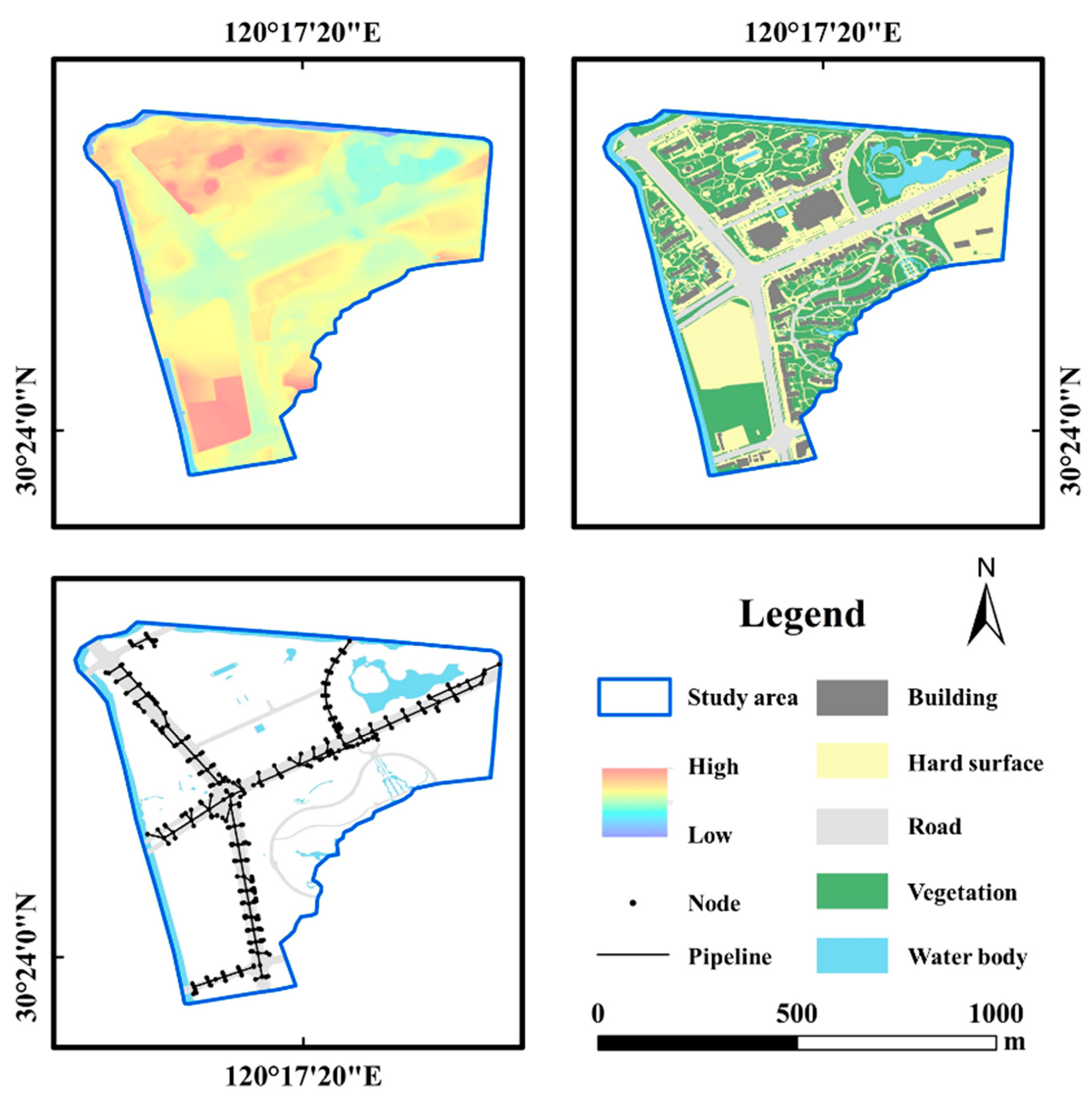
2.1. Overview of the Study Area

Waterview Community, Hangzhou City (WCHC) (120°17′1″ E–120°17′36″ E, 30°23′56″ N–30°24′27″ N), is located at the intersection of Century Avenue and Xinghe South Road, Linping District, Hangzhou, Zhejiang Province, China (Figure 1). The topography of the area is generally gentle, forming a separate catchment unit defined by major transportation arteries. The buildings in the catchment unit are predominantly used for residential purposes, with a relatively regular building layout, and the percentage of impervious surfaces is close to the percentage of pervious surfaces. The total community area is 0.50 km2.

2.2. Data Sources and Processing

2.2.1. Basic Geographic Data

The basic geographic data of this study are mainly divided into three categories: topographic data, land use data, and pipe network data. The data situation is shown in Figure 2.
  • Digital elevation data
A UAV was utilized to carry an airborne tilt camera to obtain tilt photography data of the study area, including RGB images as well as out-of-image orientation data. After camera correction and the image noise reduction process, a 3D point cloud dataset of the study area was generated. Subsequently, these point cloud data were further denoised, filtered, and categorized to extract the ground point cloud information. Based on these processed ground point cloud data, a digital elevation model (DEM) was constructed using interpolation techniques with a spatial resolution of 2 m [41].
b.
Land use data
The land use data were generated via the manual interpretation of remote sensing imagery. The images were from UAV orthophotos with a spatial resolution of 0.5 m, which meets the requirements for land use data production. Based on the study objectives, the land types in the area were categorized into five types: buildings, roads, water bodies, green spaces, and hard surfaces.
c.
Drainage network data
The stormwater network data were obtained from municipal administrations. Vectorization was carried out based on the pipeline design drawings in the area as well as the relevant planning information, converting stormwater wells into point data and pipelines into line data. The topology was determined using basic data on the stormwater wells and pipelines, i.e., a pipeline generalization was created. After generalization, the data on 309 stormwater wells and 305 pipes were obtained for the study area.

2.2.2. Precipitation Data

  • Measured rainfall data
Rain barrels were deployed in the study area to obtain measured rainfall data as model input data. Two measured rainstorms, on 25 June 2024 and 27 June 2024, were used as model simulation validation data, and the above data were used as input data for the hydrological model (Figure 3).
b.
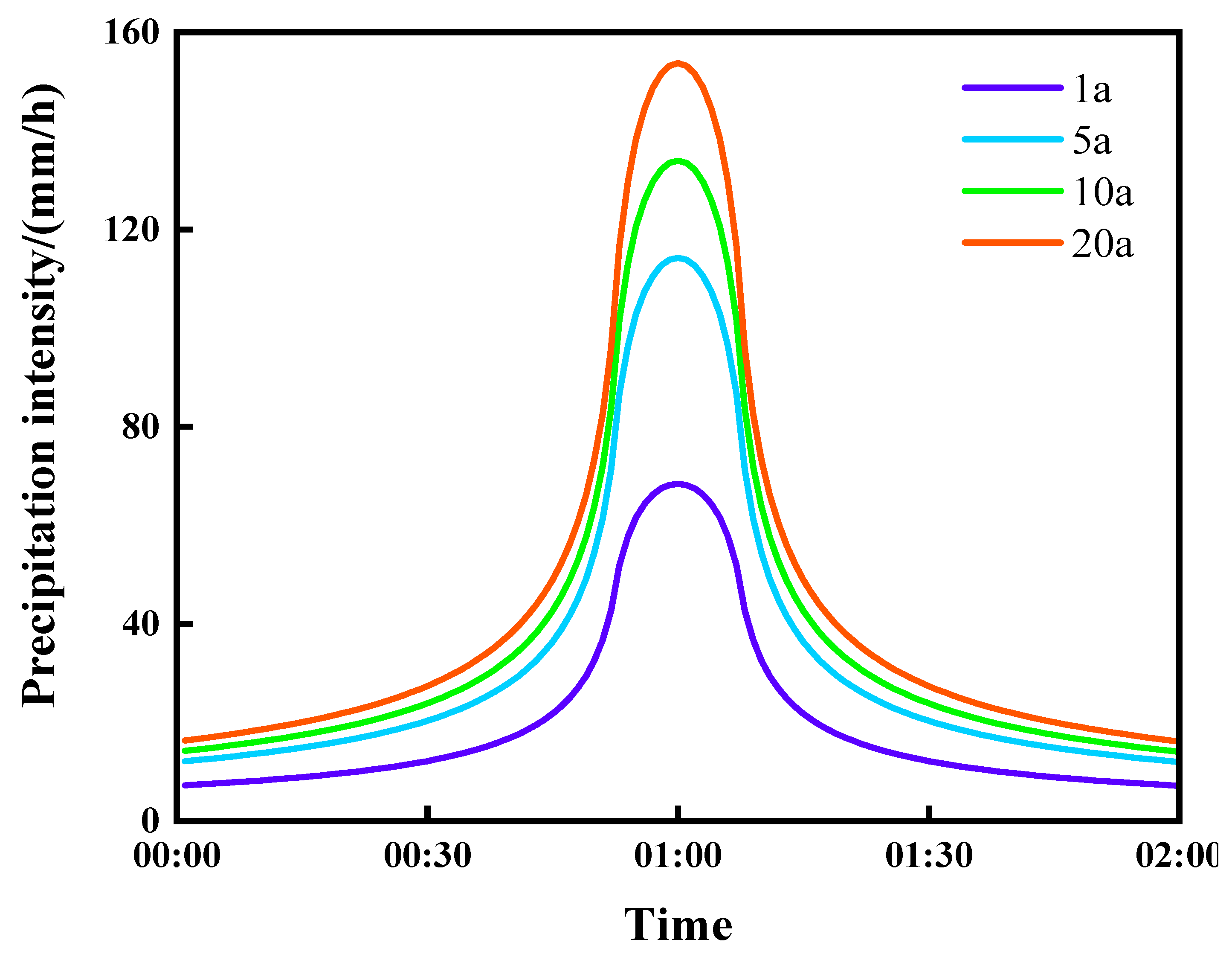
Designing storm events
The design of the storm scenario for this study utilizes the Standard for Calculating the Intensity of Rainstorms (Standard), developed by the Department of Housing and Urban–Rural Development of the Zhejiang Province. The precipitation characteristics of the study area, are based on the Chicago rain type calculations; the recommended formulas in the standard, which correspond to those used by the Linping district, are used.
q = 1455.550 × 1 + 0.958 l g P t + 5.861 0.674
where q is the precipitation intensity, L/(s·hm2); P is the return period, a; and t is the rainfall duration, min.
After transformation, the Chicago rain pattern formula is used to calculate the pre-peak and post-peak rainfall equations [42]:
i a = A 1 c t a r + b t a r + b c + 1
i b = A 1 c t b 1 r + b t b 1 r + b c + 1
where i a is the rainfall intensity before the rain peak, mm/min; i b is the rainfall intensity after the rain peak, mm/min; t a is the rainfall duration before the rain peak, min; t b is the rainfall duration before the rain peak, min; A , b , and c are the design rainfall parameters; and r is the rain peak coefficient.
In the urban precipitation rainfall pattern, the short-term peak value of precipitation exists as a greater danger to the city, and it is very easy to cause urban flooding [43]. Therefore, taking into account the comments provided by the Standard and actual precipitation in the study area, the design rainfall duration is adopted as 2 h [44,45], and the rainfall crest factor r is taken as 0.5, which is calculated according to the equation to obtain the design rainfall process for 1-year (1a), 5-years (5a), 10-years (10a), and 20-years (20a) return periods in the study area. The return period precipitation curve is shown in Figure 4.

2.3. Principles of Coupled Urban Hydrological Modeling

The coupled urban hydrological model combines a one-dimensional hydrological–hydrodynamic model with a two-dimensional hydrodynamic model. This integration is achieved through a coupled time-series based on a real-time simulation approach, where the outputs of the one-dimensional model are used as inputs for the two-dimensional model. This approach facilitates a real-time data exchange between the models; it takes into account the complexity of urban rainfall systems and improves the accuracy of flood simulations. By combining the advantages of the two models, the method improves the accuracy and comprehensiveness of the simulation results. The spatial and temporal accuracy of the model based on the principle of this chapter makes the accumulated water results obtained from this model highly feasible. Therefore, all the results used in this study were obtained from the model based on the principle of this chapter.

2.3.1. One-Dimensional Hydrological–Hydrodynamic Model

The SWMM model is based on the physical principles of hydrological processes. It simulates the operational status of urban stormwater runoff systems, outputs the overflow flow rate of each pipe node, and outputs the overflow flow rate on a node-by-node basis [46,47,48]. SWMM relies on the one-dimensional St. Venant system of equations and Manning’s equations to achieve a description of the water flow behavior in pipes or at the surface [49], and the method is computationally efficient in practical applications with better quality results.
The one-dimensional St. Venant equations are based on the continuity and momentum equations, which combine the effects of gravity, friction, etc., on the flow of water and can describe the change in water flow in space and time. The formulation of the one-dimensional St. Venant system of equations is shown below:
  • The continuity equation is used to describe the conservation of mass in the water flow:
A t + A V x = 0
2.
The momentum equation is used to describe the conservation of momentum in the water flow:
A V t + A V 2 x + g A h x = g A S f g A I
where A is the cross-sectional area, m2; t is the time, s; V is the flow velocity, m/s; x is the spatial coordinate; g is the gravitational acceleration, m/s2; h is the water level, m; S f is the frictional slope drop; and I is the lateral inflow term.

2.3.2. Two-Dimensional Hydrodynamic Model

The LISFLOOD-FP model is based on the principle of two-dimensional hydrodynamics; it takes into account a variety of factors, such as topography, rainfall, and land use, and can be used to realize the simulation of the accumulated water situation in the area where it is located by inputting the overflow volume of the overflow node [50,51,52].
The two-dimensional accumulated water diffusion simulation method of the LISFLOOD-FP model calculates the hydrodynamic dynamics of individual rectangular cells and computes the water balance on a surface whose geometry is a rectangular grid. In the simulation process, we consider not only the overall water balance, but also the water balance between neighboring rectangular grids. The principal formula is as follows:
  • Continuity equations for flow balancing:
d Q d t = Q u + Q d + Q l + Q r
2.
Uniform flow equation for neighboring image element flow:
Q i j = A i j R i j S i j 1 2 n
where Q is the total flow rate, m3/s; t is the time, s; Q u is the upstream flow rate, m3/s; Q d is the downstream flow rate, m3/s; Q l is the left flow rate, m3/s; Q r is the right flow rate, m3/s; Q i j is the flow rate of the j t h column cell in the i t h row, m3/s; A i j is the pipe cross-section of the j t h cell in the i t h row, m2; R i j is the hydraulic radius of the cell in column j of row i , m; S i j is the water surface slope of the cell in column j of row i ; and n is the Manning coefficient.

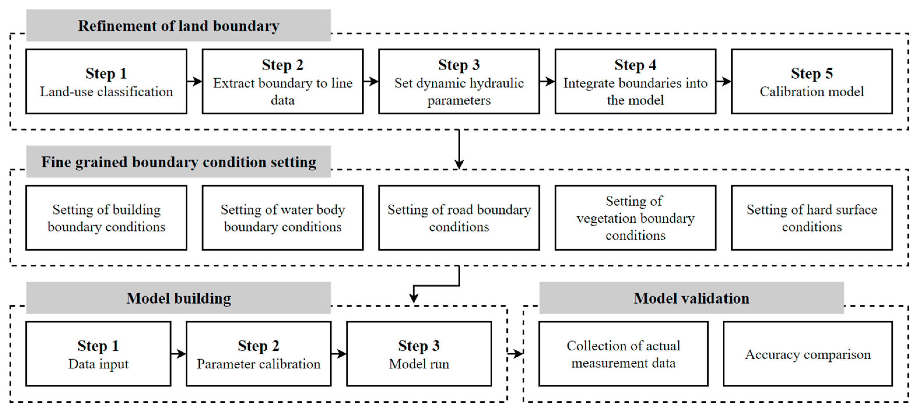
3. Materials and Methods

The methodology used in this study consists of four parts: the land boundary, fine-grained boundary condition setting, model construction, and model validation. The specific method flow is shown in Figure 5. (1) The boundaries first need to be determined based on land use classifications (buildings, water bodies, roads, vegetation, and hard surfaces); then, the boundary line data need to be extracted, and the basic hydrological parameters need to be set. (2) The boundary conditions are set according to the boundary type. (3) The data are input, the model parameters are set, and the hydrological model is run. (4) The measured data are obtained, and the model results are organized and compared. The research methodology given above aims to improve the accuracy and rationality of the urban hydrological process simulation by fine-tuning the boundary conditions of the land features.

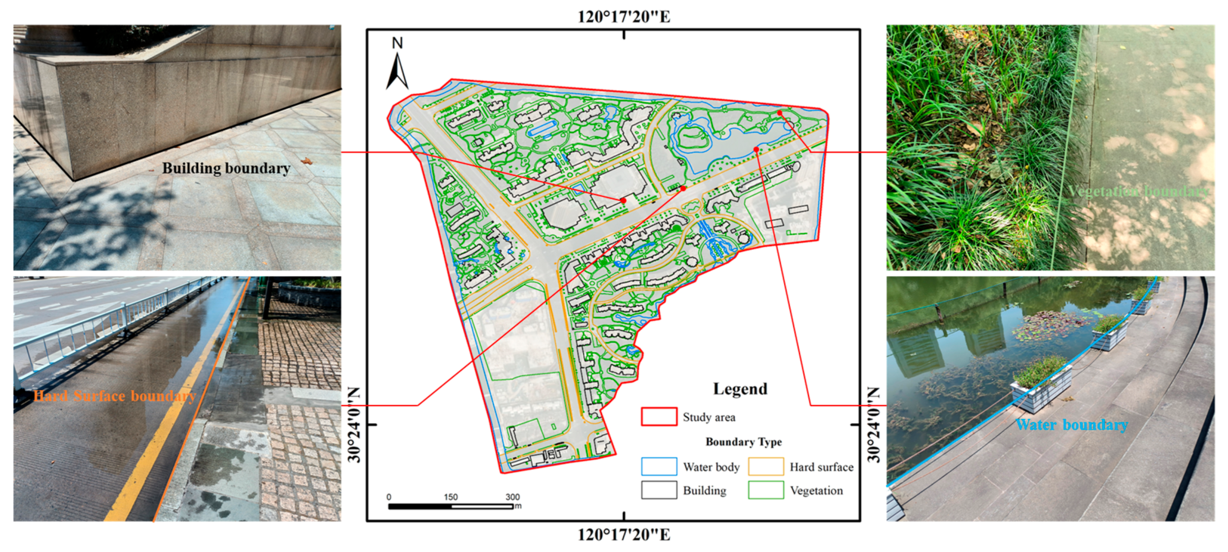
3.1. Land Feature Boundary Refinement

Urban land feature types are important input parameters for urban hydrological models. In a one-dimensional hydrodynamic model, the land feature type reflects its influence on the hydrological processes through parameters such as the runoff coefficient, infiltration rate, and Manning’s roughness coefficient [53]. Generally, the area of the land feature type is divided into impervious and pervious surfaces; the impervious surfaces, such as roads and buildings, have high runoff coefficients and low infiltration rates, resulting in the rapid formation of surface runoff from precipitation [54]. Pervious surfaces, such as green spaces and vegetated areas, have lower runoff coefficients and higher infiltration rates, which help the precipitation to infiltrate and to reduce surface runoff. In addition, Manning’s roughness coefficient is used to characterize surface roughness, which varies for different land use types and affects the velocity and flow of the water [55]. The data on land use types are usually derived from remote sensing imagery and GIS and are processed and converted into model input parameters, thereby improving the simulation accuracy and reliability of the model. The specific boundaries of the study area are shown in Figure 6.
The following are the main steps for associating terrain types with boundary conditions:
Step 1: The land use data of the study area are obtained using remote sensing images in the GIS system and then stored in a raster data format. Then, the land use data are categorized into roads, vegetation, water bodies, buildings, and hard surfaces.
Step 2: The transition areas between the land features are identified where the boundaries of the transition areas are key input data. The extracted boundaries are converted from raster data to line vector data. This transformation reduces data redundancy and allows the model to handle spatial variation in land feature types more efficiently.
Step 3: In the model, the corresponding hydrodynamic parameters for each boundary are set according to the land feature type of the boundary. These parameters can include the flow rate, flow volume, infiltration rate, etc., and should be adjusted based on the characteristics of the land use type. During the simulation process, the hydrodynamic parameters of the model are dynamically adjusted to reflect the effects of the surface features on the flow paths and confluence processes as water flows through the boundaries of the different land feature types.
Step 4: In the two-dimensional hydrodynamic model, the above-defined boundary conditions are integrated with the land use data to ensure that the model accurately captures the effects of different land feature types on the hydrological processes.
Step 5: The model is calibrated based on field observations to ensure that the model simulation results are consistent with the actual situation.

3.2. Refined Boundary Condition Setting

The refined boundary condition setting is crucial in urban hydrodynamic modeling, and the land feature types in this study include buildings, roads, water bodies, and vegetation. Due to the different hydrological characteristics between the various land feature types, the boundary conditions need to be set to characterize the hydrological parameters of the spreading process of standing water on the surface. Considering the complexity and bi-directionality of the urban surface, the bi-directional diffusion process of standing water at the surface boundary needs to be taken into account when performing the boundary condition setting. The differences in hydrological properties between the land feature types significantly affect the setting of the boundary conditions. The presence of impervious surfaces, such as buildings and roads, can alter the path and velocity of surface runoff, causing standing water to rapidly pool and spread to surrounding areas. Conversely, vegetated areas can significantly reduce surface runoff and slow down the process of the spreading of standing water due to their good permeability and retention capacity [56]. In addition, the junction of a water body with surrounding features, where the standing water enters the water body, terminates the diffusion process. Therefore, the boundary condition setting not only needs to reflect the hydrological characteristics of each land feature type, but also must take into account the transformation process of the standing water between the different land features on the surface. The complex topography and heterogeneous geological conditions at the surface further increase the difficulty of setting boundary conditions.
In this study, in order to better understand and simulate this process, Manning’s equation is used as the core equation for a boundary condition setting to help carry out a more detailed and precise boundary condition setting, using the following equations [57]:
v = 1 n R h 2 3 S 1 2
where v is the flow velocity, m/s; n is the Manning roughness coefficient; R h is the hydraulic radius, m; and S is the channel bottom slope.

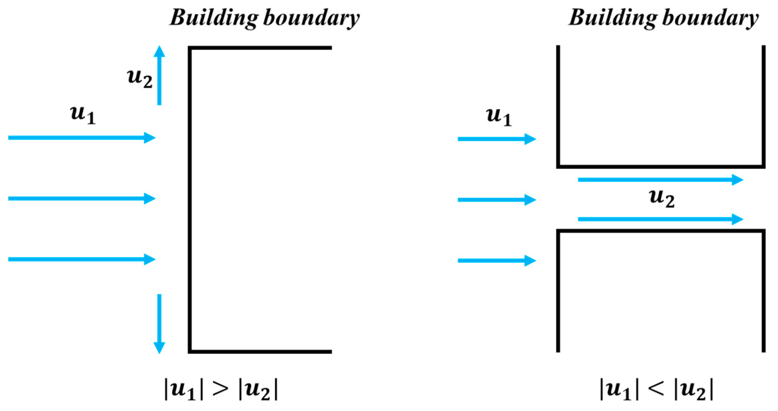
3.2.1. Setting of Building Boundary Conditions

Buildings are typical man-made features in urban areas, and they are characterized by their impenetrability. There is no need to consider the water flow inside the building boundary when setting the boundary conditions; mainly, the building variation is studied to determine the velocity field of the water flow. Buildings act as impenetrable barriers that block the surface runoff created by the spreading of surface water and change the direction of its flow. Standing water can flow along the building facade and redistribute itself around the building, resulting in the rapid pooling of standing water in the area around the building. Low-lying areas around buildings are prone to becoming places where water can pool, especially in gaps between buildings or in enclosed courtyards [58]. Once the amount of precipitation exceeds the carrying capacity of the drainage system in the above areas, the water will not be able to drain out quickly, and a significant ponding area will be formed. In addition, when standing water encounters a building, the rate of its spread is changed, with runoff slowing down somewhat at the front of the building and speeding up somewhat at the sides and rear of the building. If the building density is high, the narrow passages created between the buildings can lead to sharp changes in localized flow velocities. The impact of construction on the spread of standing water is shown in Figure 7.
The following equations characterize the receipt and expenditure of water around a building, taking into account the blocking and redistributing effects of the building on the flow:
( ρ u ) t + ρ u u + p = ρ g
where ρ is the density of water; u is the velocity field of the water flow; g is the acceleration of gravity, m/s2; and t is the time, s.
Buildings often have a distance from the ground surface due to their own height, and standing water does not form within the building boundaries; thus, the building boundaries are unidirectional.

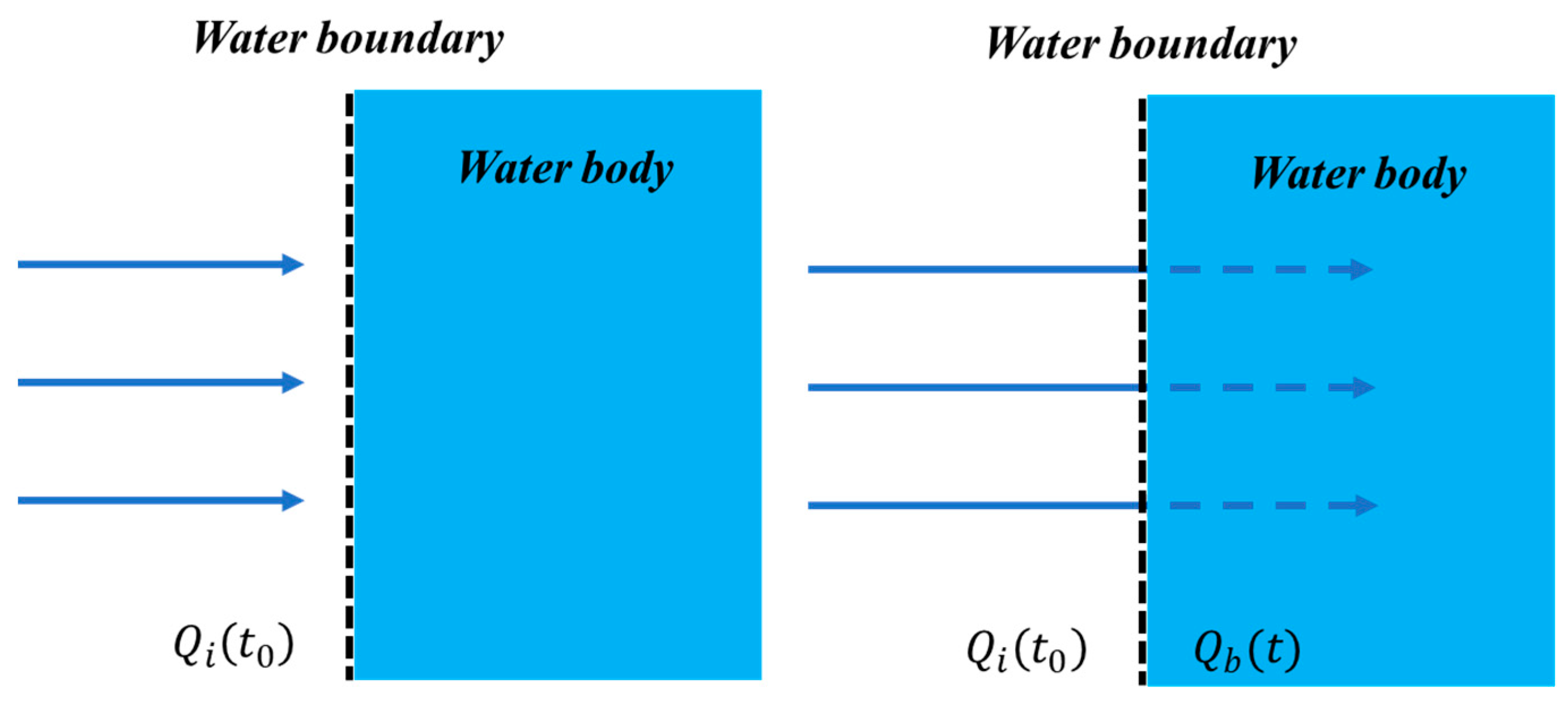
3.2.2. Setting of Water Body Boundary Conditions

In this study, the water level change is not considered when performing the boundary condition setting of the water body, which is regarded as an open boundary; thus, there is no need to consider the water flow inside the building boundary during the boundary condition setting. Standing water enters the water body through other boundaries, and the model needs to accurately describe the magnitude of the standing water flow at the inlet and its time-series to reflect the actual precipitation or surface runoff. Once standing water enters a water body, the total capacity of the water body and the potential risk of overflow need to be considered, even though the water level remains relatively stable. Diffusion equations within the water body should also be included to depict the distribution of standing water in the water body. The method can ignore downstream boundary conditions and deal with the subsequent flow or dispersion of standing water. With this setup, the model is able to efficiently simulate the spreading behavior of standing water in urban environments, providing important information about the direction of the standing water flow and spreading patterns under long-term average conditions, even without tracking the instantaneous water level changes [59]. This simplified approach is suitable for scenarios where the impact of standing water needs to be quickly assessed; however, the impact of water level changes on the spread of standing water needs to be reassessed in the face of extreme precipitation or the near saturation of the water body. The interaction of the water body boundaries with standing water is shown in Figure 8.
The following equations characterize the receipt and expenditure of water around a building, taking into account the blocking and redistributing effects of the building on the flow:
V t = V t 0 + i = 1 N Q i t Q b t
where V t is the total volume of water at time t , m3; V t 0 is the total volume of water at the initial moment, m3; Q i t is the overflow volume generated at time t , m3/s; and Q b t is the total volume of water flowing into the boundary of the inlet water body at time t , m3/s.

3.2.3. Setting of Road Boundary Conditions

Road surfaces also play a key role in the urban hydrological cycle. Roadway surfaces typically have low roughness coefficients (typically less than 0.4) [60], which means that water flows more fluidly over their surfaces and tends to create rapid surface runoff. Roadway surfaces have little or no retention capacity, and stormwater is barely retained on the surface and flows rapidly along the roadway surface. Due to the lack of infiltration channels and the poor permeability of the road surface, most of the precipitation cannot be converted into underground runoff through infiltration, but directly forms surface runoff. In addition, roadway designs are often sloped to facilitate the rapid drainage of standing water, which increases the hydraulic radius and makes it easier for water to pool and move quickly. The design of roadway bottom slopes helps to direct the direction of runoff and has a significant effect on runoff rates despite their low degree of undulation.
By synthesizing the hydrological characteristics of the road using Equation (8), the following settings were determined for the road boundary conditions (Table 1).

3.2.4. Setting of Vegetation Boundary Conditions

The significant reduction in surface runoff by vegetation is a key hydrological process in the urban hydrological cycle. Research data suggest that surface runoff can be reduced by up to 80% or more in areas with good vegetation cover [61]; this percentage varies depending on the vegetation type, density, soil conditions, and intensity and duration of precipitation. Vegetation surfaces have high roughness coefficients, usually between 0.05 and 0.15 [62], and the water flow encounters greater resistance. The vegetation root system improves the soil structure, increases the soil permeability, and promotes the rapid infiltration of rainwater into underground runoff, thereby significantly reducing surface runoff. In addition, the hydraulic radius is influenced by the density of vegetation and the depth of standing water, while the bottom slopes are likely to be those with a high degree of undulation in areas covered with vegetation. Through the retention effect of vegetation, rainwater is intercepted by the leaves and branches of plants and subsequently drips slowly or evaporates, effectively reducing the amount of water that immediately forms surface runoff. Transpiration by plants releases absorbed water back into the atmosphere, further reducing the amount of water available to flow at the surface. Surface vegetation cover also mitigates the direct impact of rainfall on the soil, reducing soil erosion and indirectly inhibiting the formation of surface runoff. Based on fieldwork, most of the vegetation in the study area is man-made, and there are other non-vegetated features in the vegetated areas; thus, the coverage is about 80 percent.
By synthesizing the hydrological characteristics of the vegetation using Equation (8), the following settings were determined for the vegetation boundary conditions (Table 2).

3.2.5. Setting of Hard Surface Boundary Conditions

Hard surfaces play an important role in the urban hydrological cycle. Such surfaces usually have a low roughness coefficient, which means that water flows move faster over the surface. Hard surfaces with roads lack infiltration channels, surface permeability is poor, and most of the precipitation cannot infiltrate and becomes surface runoff. Hard surfaces have little or no retention; rainwater is barely retained on the surface, but rapidly forms surface runoff. In addition, the hydraulic radius on hard surfaces is relatively large, which makes it easier for water to pool and move quickly [63]. Bottom slopes on hard surfaces also affect the rate and direction of runoff, but are less undulating than in vegetated areas. Based on fieldwork, the study area has an approximately 90 percent hard surface coverage.
By synthesizing the hydrological characteristics of the hard surface using Equation (8), the following settings were determined for the hard surface boundary conditions (Table 3).

3.3. Model Building

In this study, three scenarios (original, rough depiction, and refined depiction) were set up for accuracy validation and urban hydrological analysis.
Original: This scenario only uses the original 2 m resolution DEM without any additional refinement of the boundary conditions. In this scenario, the model can only reflect the hydrological situation under the original surface. The surface type is not taken into account in the simulation process, i.e., uniform infiltration values and friction are used.
Rough depiction: This scenario is a preliminary simplification of the original surface model. It depicts the buildings and roads within the urban neighborhood, and only sets the hydrological process conditions for the buildings and roads, and does not depict other urban land feature types.
Refined depiction: This scenario depicts the original surface model with boundaries based on the land feature type and hydrologic process conditions based on the land feature type. This scenario captures the details of roads, buildings, vegetation, water bodies, and other land features more accurately, and has a higher simulation accuracy. The hydrological characteristics of each feature are taken into account in the simulation process, and parameters such as infiltration values and friction are set according to the type of land feature.
Step 1: Data Entry
A modified digital elevation model (DEM) is used to accurately reflect urban topographic features, including the effects of man-made features. Based on the corrected DEM and drainage facility locations, the model determines a reasonable catchment delineation by drawing and adjusting Tyson polygons to ensure a realistic representation of water flow paths. In addition, to accurately simulate hydrological processes, the model needs to receive high-quality precipitation data, including single-point rainfall station data and surface precipitation data, and to ensure that the temporal and spatial resolution of these data meets the modeling needs.
Step 2: Parameter rate setting
The input parameters of the model are determined upfront and are mainly categorized into deterministic and uncertain parameters. The measured sensor data are collected, and the parameters are validated and optimized based on the sensor data to improve the model simulation accuracy. Afterwards, the hydrological parameters formed according to the boundary conditions are entered to complete parameter rate determination.
Step 3: Model Running
The simulation duration and time step are set for the model. Once the settings are completed, the running of the model can be started. When the model has finished running, the output is obtained.

3.4. Model Validation

To assess the accuracy of the coupled model in predicting the accumulated water due to precipitation, three precipitation events, 11 May, 30 May, and 9 June 2024, were selected as case studies. During these three events, we conducted site surveys, documented in detail the actual areas of standing water that formed, and compared this information to the model’s predictions. Specifically, we field labeled all the observed locations of accumulated water and then matched these locations to areas of accumulated water predicted by the model as a means of determining the accuracy of the model predictions. The results show that for all three precipitation events, the prediction accuracy of the coupled model exceeded 90%, as shown in Table 4. In particular, the model achieved a prediction accuracy of 92.6% for the 11 May 2024 precipitation event, which was the highest value among the three tests, further demonstrating the efficiency and accuracy of the coupled model in dealing with this type of prediction problem.

4. Results

4.1. Analysis of Model Simulation Results

In this study, water depth variation curves and measured water depth variation curves were obtained under three boundary condition scenarios based on data obtained from buried water detectors installed in the study area. The measuring accuracy of the detector is 0.1 cm, and the time resolution is 10 min. As can be seen in Figure 9, the three boundary condition scenarios in the 20240625 event are more consistent with the measured waterlogging depth change curve, and the waterlogging peaks of the simulated boundary condition scenarios are all around 8:30 min; furthermore, the overall trend of the waterlogging changes are more correctly described. The refined depiction scenario’s accumulated water curve has a lower overall depth and is closer to the measured accumulated water curve, with the slowest rate of accumulated water and receding water. The three boundary condition scenarios have the same trend as the measured accumulated water depth change curves in the 20240627 event. The accumulated water curve for the refined depiction scenario was also closer to the measured curve in that field, and the overall depth was higher in the rough depiction scenario. Overall, the refined depiction DEM scenario has the closest accumulated water curve in relation to the measured curve, while the refined depiction scenario has the largest accumulated water difference, and the original scenario is in between the two scenarios.
In this study, the average absolute error between the depth and the measured depth of the standing water was obtained for the three scenarios (Table 5). In the refined depiction scenario, the average absolute errors of the 20240625 event and the 20240627 event were 0.60 cm and 0.49 cm, respectively, and the overall error was 0.54 cm, which was the smallest average absolute error among the three scenarios. In the rough depiction scenario, the mean absolute errors of the 20240,25 event and the 20240627 event were 1.35 cm and 1.33 cm, respectively, and the overall error was 1.34 cm, which was the largest mean absolute error among the three scenarios. In the original scenario, the average absolute errors of the 20240625 event and the 20240627 event were 0.82 cm and 0.72 cm, respectively, and the overall error was 0.77 cm, with an average absolute error between the other two scenarios.

4.2. Comparative Analysis of Model Performance Before and After Boundary Condition Refinement

In this study, based on the regional precipitation characteristics, four precipitation return periods of 1a, 5a, 10a, and 20a were selected to be simulated using the coupled model for the three boundary condition scenarios of the original simulation, rough depiction, and refined depiction (Figure 10). The three boundary condition scenarios in the 1a return period simulated relatively similar results for accumulated water, with the main points of accumulated water being on the eastern and southern roadways. In the refined depiction scenario, the simulated accumulated water was smaller in extent, more discrete in distribution, deeper in depth, and was concentrated at the roadside. All three boundary condition scenarios simulated an increase in the extent of the accumulated water during the 5a return period, with the refined depiction simulating a gradual patching of the accumulated water and the rough depiction scenario simulating a larger extent of the accumulated water compared to the original simulation. The difference between the original and the rough depiction scenarios simulating the accumulated water results increased on the eastern arterials over the 10a return period. The simulation results for the rough depiction scenario were significantly larger than those for the original scenario, and the simulated extent of the accumulated water in the refined depiction scenario grew steadily on the main roadway. Over the 20a return period, the simulated accumulated water results for the rough depiction scenario were significantly larger in range than the simulated accumulated water results for the other scenarios, and the simulated accumulated water results for the refined depiction scenario were the smallest in range. From the simulated accumulated water results for the three boundary condition scenarios during the different precipitation return periods, the rough depiction results showed a wider spread of accumulated water due to the fact that the only boundary condition limitations were the road, the buildings, and the hard surface; furthermore, the lack of limitations due to other boundaries allowed the accumulated water to invade into other land features. Since the original DEM data were used, the accumulated water was less constrained, and its spread was more susceptible to the original surface undulation conditions. The refined depiction scenario had the smallest range of accumulated water, which did not intrude into buildings or water bodies, and the simulation results were more in line with the actual situation because of the consideration of factors such as the infiltration of vegetation and changes in the water velocity.
Figure 11 shows the simulated accumulated water areas for the original DEM, rough depiction DEM, and refined depiction DEM boundary condition scenarios for the four precipitation return periods. During the 1a return period, the difference in the accumulated water areas between the three boundary condition scenarios was small, with the rough depiction having the largest accumulated water area of 15,580 m2 and the refined depiction having the smallest accumulated water area of 10,616 m2. The difference in the area of the accumulated water between the original and the rough depiction and refined depiction increased during the 5a return period, with differences of 3372 m2 and 7424 m2, respectively. The difference in the area of the accumulated water between the original and the rough depictions and refined depictions further increased during the 10a return period, with differences of 3664 m2 and 8796 m2, respectively. The difference in the accumulated water area between the rough depiction and the refined depiction peaked at 10,208 m2 for the 20a return period. Overall, the rough depiction had the largest simulated area of accumulated water for the same return period, while the refined depiction had the smallest. As the return period increased, the difference in the simulated accumulated water area between the original and the rough depiction gradually stabilized, while the difference in the simulated accumulated water area in the refined depiction gradually increased.

4.3. Study of Accumulated Water Dynamics After Refinement of Boundary Conditions

Based on the modeling results, this study obtained the resultant maps of the accumulated water spreading direction for two precipitation events after the boundary condition refinement (Figure 12). During the 20240625 precipitation event, the accumulated water was mainly distributed on the road, and the direction of flow of the accumulated water inside the boundary was mainly influenced by the topography, with the water flowing from high to low, whereas the direction of the flow of the accumulated water around the boundary was influenced by the boundary conditions, with the direction of flow changing to some extent. During the 20240627 precipitation event, the main accumulated water situation was the same as that of the 20240625 precipitation event in terms of distribution on the road; however, due to the large amount of precipitation in this area, the accumulated water spread to other land features within the boundary. At the same time, the accumulated water flow within the boundary of the interior followed the physical laws of the boundary, and the accumulated water on the boundary was affected by different boundary conditions. In terms of the direction of the accumulated water, when the accumulated water interacted with the building boundary, its direction was perpendicular or opposite to the original direction. After the water interacted with the water body boundary, the diffusion process ended as the accumulated water entered the water body. When the accumulated water interacted with the vegetation, roads, and hard surface boundaries, its direction changed irregularly.
In addition, the average diffusion rate of the accumulated water at the checkpoints was obtained from the results of the accumulated water dynamics, and it was found that there were significant differences in the accumulated water within and on the boundaries (Table 6). To ensure the scientific validity of the results verified by the checkpoints, a total of 10 checkpoints were set up in the study area, five distributed within the boundaries and five at the boundaries, where the checkpoints at the boundaries were also considered as far as possible for the boundary types. In general, the diffusion velocity of the accumulated water inside the boundary was higher than that on the boundary; the average diffusion velocity of the accumulated water inside the boundary was 0.057 m/s, while the average diffusion velocity of the accumulated water on the boundary was 0.037 m/s, which was consistent with the boundary condition setting. Within the boundary, the flow rates of the accumulated water on the different land features also showed some differences, with the fastest diffusion rate being that of the accumulated water on hard surfaces, at 0.078 m/s, and the slowest diffusion rate being that of the accumulated water on vegetation at 0.032 m/s. At the boundary, the diffusion rate of the accumulated water at the checkpoints fluctuated, but was below 0.05 m/s overall.

5. Discussion

5.1. Influence of Boundary Conditions on the Accuracy and Extent of Simulation of Accumulated Water

It is shown that in the three boundary condition scenarios of the refined depiction, original simulation, and rough depiction, the refined depiction scenario provides the highest simulation accuracy, with mean absolute errors of 0.6 cm and 0.49 cm for the two precipitation events. These are significantly lower than those of 1.35 cm and 1.33 cm in the rough depiction scenario with mean absolute errors of 0.6 cm and 0.49 cm for the two precipitation events, which are significantly lower than 1.35 cm and 1.33 cm in the rough depiction scenario. This means that the refined boundary conditions can more accurately reproduce real accumulated water conditions. In addition, the simulated accumulated water area in the rough depiction scenario is significantly larger than that of the other two scenarios for different precipitation return periods (1a, 5a, 10a, and 20a) and the difference in the accumulated water area with the refined depiction scenario peaks, particularly during the 20a return period. Model resolution is also important for boundary condition setting, as high-resolution models can capture finer feature characteristics and thus describe boundary conditions more accurately. Especially since there are a large number of irregular boundaries in cities, low-resolution models can lead to model distortion, which in turn affects model accuracy [64,65]. However, it is also important to consider the increase in the computational cost for high-resolution modeling as well as the difficulty of data acquisition. Therefore, the model resolution has a large impact on the model results, and the selection of the appropriate resolution should be based on the study area and the research needs. Mason et al. explored the enhancement of model accuracy through the correlation of SAR and model data [66], and Hou et al. proposed to increase the temporal resolution of model input storm data to improve the model accuracy [67]. All of the above studies are very inspiring for this study as they improve the accuracy of urban hydrological modeling from a scientific point of view, but the related studies are less involved in the simulation of the accumulated water with fine depiction of boundaries, which is the key to this study. Based on the high-resolution terrain model and land use data, this study significantly improves the accuracy of the simulation and reduces the average absolute error by realizing a fine description of the urban terrain and feature characteristics. Compared with the traditional methods, this study enhances the robustness and reliability of the model, thus providing a new method to improve the simulation accuracy of hydrological models.

5.2. Influence of Boundary Conditions on the Dynamic Behavior of Accumulated Water

This study also analyzed the effect of boundary conditions on the dynamic behavior of accumulated water. During the 20240625 and 20240627 precipitation events, the accumulated water was primarily distributed over roadways, and the direction of flow was influenced by topography and boundary conditions. In particular, during the heavier precipitation events of 20240627, the accumulated water not only flowed along the roadway, but also spread out within other land feature boundaries, where the interactive behavior of the boundaries between different land feature types occurred. In addition, the accumulated water spreading velocity results were consistent with the previous land feature boundary condition settings. In addition, it was found that the flow rate of the accumulated water within the boundary was higher than the flow rate over the boundary, with the fastest diffusion of the accumulated water over hard surfaces and the slowest diffusion of the accumulated water over vegetation. The average spreading rate of the accumulated water between the two precipitation events showed that there was no significant relationship between the magnitude of precipitation and the spreading rate. Both Yang et at. and Li et at. validate the accuracy of the model with the measured data, which inspired this study [68,69]. However, the above studies are lacking in terms of testing the dynamics of hydrological models. Since this study focuses on the effect of boundary refinement on hydrological processes and is highly sensitive to changes in hydrological processes at the boundary as well as within the boundary, a special test of dynamics was made in this study. The results show that the refined boundary conditions not only improve the simulation of the static distribution of accumulated water, but also simulate the dynamic flow This study not only focuses on the static distribution of accumulated water, but also explores its dynamic behavior, such as the flow direction and diffusion rate of the accumulated water, which provides a new perspective for understanding the interactive behavior of accumulated water under different types of feature boundary conditions, and a new method for assessing the accuracy of the model more comprehensively.

6. Conclusions

WCHC, Hangzhou City, was taken as the study area. The boundaries of the land features in the area were refined, and three comparative scenarios (original, rough depiction, and refined depiction) were constructed. The coupled model was used to obtain the simulation of the accumulated water in the study area for the real scenarios (20240625 and 20240627) and the designed precipitation scenarios (1a, 5a, 10a, and 20a). They were compared with the actual accumulated water data, and the simulation results were analyzed. The main conclusions are as follows:
(1)
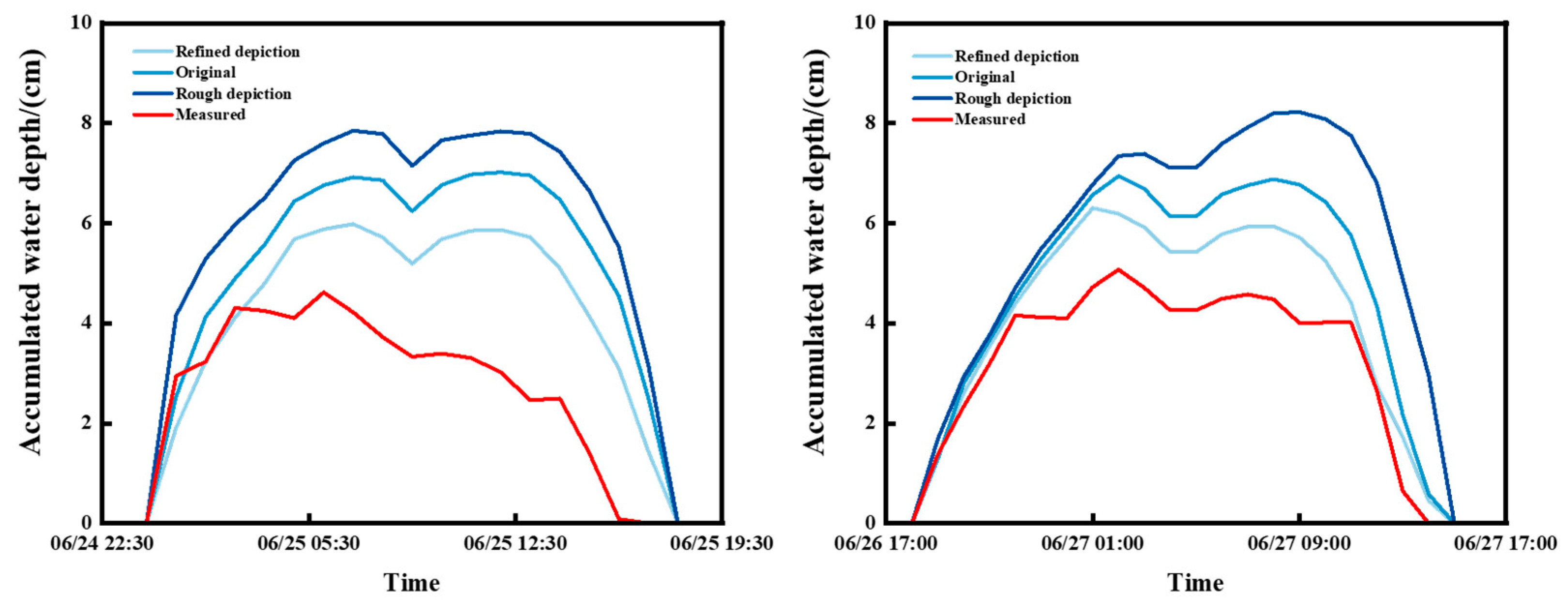
The accumulated water depth change curves for three boundary condition scenarios of the refined depiction, original simulation, and rough depiction were compared using the measured precipitation as the validation data. The results show that the accumulated water curves of the refined depiction scenarios for the 20240625 and 20240627 precipitation events were the closest to the measured curves, with mean absolute errors of 0.60 cm and 0.49 cm, respectively, and the smallest overall errors. The rough depiction scenarios had the largest errors of 1.35 cm and 1.33 cm, respectively. From the results, it can be seen that compared with the original and rough depiction, the results of the refined depiction have higher accuracy, which is improved by 28.1% and 16.5%, respectively. Therefore, it is proved that the model after the refined boundary can simulate the real hydrological situation of the city under heavy rainfall conditions.
(2)
Three boundary condition scenarios, the refined depiction, original simulation, and rough depiction, were simulated over four precipitation return periods, 1a, 5a, 10a, and 20a. The results show that the simulated accumulated water area in the rough depiction scenario was significantly larger than that of the other two scenarios as the return period increased. The refined depiction scenario had the smallest extent of accumulated water and was more realistic because it took into account factors such as vegetation infiltration and changes in the water velocity to avoid the excessive spreading of accumulated water to features where it should not be. The difference in the average accumulated water area between the refined and original scenarios amounted to 21.45%, while the difference in the average accumulated water area in the rough depiction scenario amounted to 32.18%. Overall, the refined depiction scenario provided the most accurate simulation results for the extent of the accumulated water during each return period.
(3)
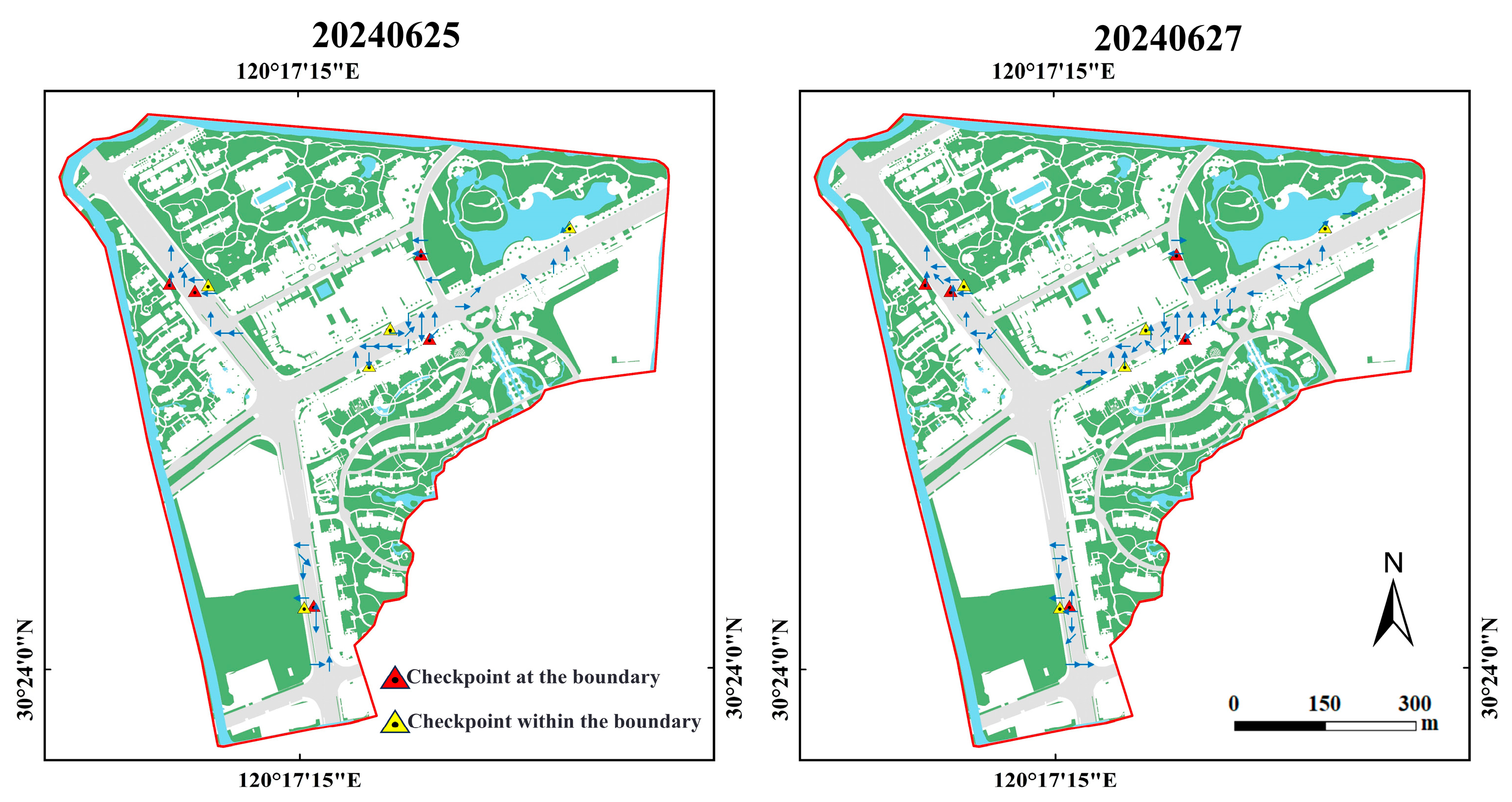
According to the analysis of the dynamic process of the accumulated water, it was mainly distributed along the road, and the flow direction of the accumulated water inside the boundary was influenced by the topography, flowing from high to low; however, the accumulated water around the boundary was influenced by the boundary conditions, and the flow direction was changed. In particular, during the heavy precipitation event of 20240627, the accumulated water spread within the boundaries of the other land features, and the direction of the accumulated water after interacting with different boundaries showed diverse changes. It was also found that the flow rate of the accumulated water inside the boundary was higher than that on the boundary, and that the fastest diffusion of the accumulated water was on the hard surface, while the slowest diffusion of the accumulated water was on the vegetation. These results show that refined boundary conditions not only affect the static distribution of accumulated water, but also significantly influence the dynamic behavior of accumulated water.

Author Contributions

Conceptualization, C.C.; methodology, C.C. and Y.Z.; software, C.C.; validation, Y.L. and Z.T.; formal analysis, Y.L. and Y.Z.; investigation, P.W.; resources, T.H.; data curation, C.C.; writing—original draft preparation, C.C.; writing—review and editing, T.H. and P.W.; visualization, C.C.; supervision, P.W.; project administration, P.W.; funding acquisition, T.H. All authors have read and agreed to the published version of the manuscript.

Funding

This work was supported by the National Natural Science Foundation of China (Grant 42471102).

Data Availability Statement

Data will be made available on request.

Acknowledgments

The authors appreciate the editors and anonymous reviewers for their valuable comments and suggestions.

Conflicts of Interest

The authors declare no conflicts of interest.

References

  1. Cristiano, E.; ten Veldhuis, M.-C.; Van De Giesen, N. Spatial and temporal variability of rainfall and their effects on hydrological response in urban areas—A review. Hydrol. Earth Syst. Sci. 2017, 21, 3859–3878. [Google Scholar]
  2. Rezaei, A.R.; Ismail, Z.B.; Niksokhan, M.H.; Ramli, A.H.; Sidek, L.M.; Dayarian, M.A. Investigating the effective factors influencing surface runoff generation in urban catchments—A review. Desalin. Water Treat. 2019, 164, 276–292. [Google Scholar]
  3. Williams, E.S.; Wise, W.R. Hhydrologic impacts of alternative approaches to storm water management and land development 1. JAWRA J. Am. Water Resour. Assoc. 2006, 42, 443–455. [Google Scholar]
  4. Wang, Y.; Zhang, X.; Xu, J.; Pan, G.; Zhao, Y.; Liu, Y.; Liu, H.; Liu, J. Accumulated impacts of imperviousness on surface and subsurface hydrology—Continuous modelling at urban street block scale. J. Hydrol. 2022, 608, 127621. [Google Scholar] [CrossRef]
  5. Shen, Y.; Morsy, M.M.; Huxley, C.; Tahvildari, N.; Goodall, J.L. Flood risk assessment and increased resilience for coastal urban watersheds under the combined impact of storm tide and heavy rainfall. J. Hydrol. 2019, 579, 124159. [Google Scholar]
  6. Xu, H.; Gao, J.; Yu, X.; Qin, Q.; Du, S.; Wen, J. Assessment of Rainstorm Waterlogging Disaster Risk in Rapidly Urbanizing Areas Based on Land Use Scenario Simulation: A Case Study of Jiangqiao Town in Shanghai, China. Land 2024, 13, 1088. [Google Scholar] [CrossRef]
  7. Wu, X.; Yu, D.; Chen, Z.; Wilby, R.L. An evaluation of the impacts of land surface modification, storm sewer development, and rainfall variation on waterlogging risk in Shanghai. Nat. Hazards 2012, 63, 305–323. [Google Scholar]
  8. Zhao, Y.; Rong, Y.; Liu, Y.; Lin, T.; Kong, L.; Dai, Q.; Wang, R. Investigating Urban Flooding and Nutrient Export under Different Urban Development Scenarios in the Rouge River Watershed in Michigan, USA. Land 2023, 12, 2163. [Google Scholar] [CrossRef]
  9. Pekel, J.-F.; Cottam, A.; Gorelick, N.; Belward, A.S. High-resolution mapping of global surface water and its long-term changes. Nature 2016, 540, 418–422. [Google Scholar] [CrossRef]
  10. Zhang, H.; Chen, Y.; Zhou, J. Assessing the long-term impact of urbanization on run-off using a remote-sensing-supported hydrological model. Int. J. Remote Sens. 2015, 36, 5336–5352. [Google Scholar]
  11. Bian, G.; Wang, G.; Chen, J.; Zhang, J.; Song, M. Spatial and seasonal variations of hydrological responses to climate and land-use changes in a highly urbanized basin of Southeastern China. Hydrol. Res. 2021, 52, 506–522. [Google Scholar]
  12. Jahan, K.; Pradhanang, S.M.; Bhuiyan, M.A.E. Surface runoff responses to suburban growth: An integration of remote sensing, GIS, and curve number. Land 2021, 10, 452. [Google Scholar] [CrossRef]
  13. Zhai, H.; Lv, C.; Liu, W.; Yang, C.; Fan, D.; Wang, Z.; Guan, Q. Understanding spatio-temporal patterns of land use/land cover change under urbanization in Wuhan, China, 2000–2019. Remote Sens. 2021, 13, 3331. [Google Scholar] [CrossRef]
  14. Hassan, M.M. Monitoring land use/land cover change, urban growth dynamics and landscape pattern analysis in five fastest urbanized cities in Bangladesh. Remote Sens. Appl. Soc. Environ. 2017, 7, 69–83. [Google Scholar] [CrossRef]
  15. Hu, P.; Li, F.; Sun, X.; Liu, Y.; Chen, X.; Hu, D. Assessment of land-use/cover changes and its ecological effect in rapidly urbanized areas—Taking Pearl River Delta urban agglomeration as a case. Sustainability 2021, 13, 5075. [Google Scholar] [CrossRef]
  16. Hu, S.; Fan, Y.; Zhang, T. Assessing the effect of land use change on surface runoff in a rapidly urbanized city: A case study of the central area of Beijing. Land 2020, 9, 17. [Google Scholar] [CrossRef]
  17. Zimmermann, E.; Bracalenti, L.; Piacentini, R.; Inostroza, L. Urban flood risk reduction by increasing green areas for adaptation to climate change. Procedia Eng. 2016, 161, 2241–2246. [Google Scholar]
  18. Chithra, S.; Nair, M.H.; Amarnath, A.; Anjana, N. Impacts of impervious surfaces on the environment. Int. J. Eng. Sci. Invent. 2015, 4, 27–31. [Google Scholar]
  19. Yao, L.; Wei, W.; Chen, L. How does imperviousness impact the urban rainfall-runoff process under various storm cases? Ecol. Indic. 2016, 60, 893–905. [Google Scholar]
  20. Archer, N.; Bonell, M.; Coles, N.; MacDonald, A.; Auton, C.; Stevenson, R. Soil characteristics and landcover relationships on soil hydraulic conductivity at a hillslope scale: A view towards local flood management. J. Hydrol. 2013, 497, 208–222. [Google Scholar] [CrossRef]
  21. Balugani, E.; Lubczynski, M.; Reyes-Acosta, L.; Van Der Tol, C.; Francés, A.; Metselaar, K. Groundwater and unsaturated zone evaporation and transpiration in a semi-arid open woodland. J. Hydrol. 2017, 547, 54–66. [Google Scholar] [CrossRef]
  22. Suprayogo, D.; van Noordwijk, M.; Hairiah, K.; Meilasari, N.; Rabbani, A.L.; Ishaq, R.M.; Widianto, W. Infiltration-friendly agroforestry land uses on volcanic slopes in the Rejoso Watershed, East Java, Indonesia. Land 2020, 9, 240. [Google Scholar] [CrossRef]
  23. Bai, T.; Mayer, A.L.; Shuster, W.D.; Tian, G. The hydrologic role of urban green space in mitigating flooding (Luohe, China). Sustainability 2018, 10, 3584. [Google Scholar] [CrossRef] [PubMed]
  24. Yang, J.-L.; Zhang, G.-L. Water infiltration in urban soils and its effects on the quantity and quality of runoff. J. Soils Sediments 2011, 11, 751–761. [Google Scholar] [CrossRef]
  25. Zhang, B.; Xie, G.; Zhang, C.; Zhang, J. The economic benefits of rainwater-runoff reduction by urban green spaces: A case study in Beijing, China. J. Environ. Manag. 2012, 100, 65–71. [Google Scholar] [CrossRef]
  26. Sitharam, T. Efficacy of coastal reservoirs to address India’s water shortage by impounding excess river flood waters near the coast. J. Sustain. Urban. Plan. Prog. 2017, 2, 49–54. [Google Scholar] [CrossRef]
  27. Lee, E.; Lee, D.; Kim, S.; Lee, K. Design strategies to reduce surface water flooding in a historical district. J. Flood Risk Manag. 2018, 11, S838–S854. [Google Scholar] [CrossRef]
  28. Munir, B.A.; Iqbal, J. Flash flood water management practices in Dera Ghazi Khan City (Pakistan): A remote sensing and GIS prospective. Nat. Hazards 2016, 81, 1303–1321. [Google Scholar] [CrossRef]
  29. Rodriguez, F.; Andrieu, H.; Morena, F. A distributed hydrological model for urbanized areas–Model development and application to case studies. J. Hydrol. 2008, 351, 268–287. [Google Scholar] [CrossRef]
  30. Salvadore, E.; Bronders, J.; Batelaan, O. Hydrological modelling of urbanized catchments: A review and future directions. J. Hydrol. 2015, 529, 62–81. [Google Scholar] [CrossRef]
  31. Jantz, C.; Drzyzga, S.; Maret, M. Calibrating and validating a simulation model to identify drivers of urban land cover change in the Baltimore, MD metropolitan region. Land 2014, 3, 1158–1179. [Google Scholar] [CrossRef]
  32. Ma, Z.; Yao, R.; Sun, P.; Zhuang, Z.; Ge, C.; Zou, Y.; Lv, Y. Quantitative evaluation of runoff simulation and its driving forces based on hydrological model and multisource precipitation fusion. Land 2023, 12, 636. [Google Scholar] [CrossRef]
  33. Patel, R. Mathematical Model of the Kaipara Catchment. Doctoral Dissertation, The University of Auckland, Auckland, New Zealand, 1981. [Google Scholar]
  34. Granata, F.; Gargano, R.; De Marinis, G. Support vector regression for rainfall-runoff modeling in urban drainage: A comparison with the EPA’s storm water management model. Water 2016, 8, 69. [Google Scholar] [CrossRef]
  35. Flint, L.E.; Flint, A.L.; Thorne, J.H.; Boynton, R. Fine-scale hydrologic modeling for regional landscape applications: The California Basin Characterization Model development and performance. Ecol. Process. 2013, 2, 25. [Google Scholar] [CrossRef]
  36. Raza, A.; Ahrends, H.; Habib-Ur-Rahman, M.; Gaiser, T. Modeling approaches to assess soil erosion by water at the field scale with special emphasis on heterogeneity of soils and crops. Land 2021, 10, 422. [Google Scholar] [CrossRef]
  37. Feng, B.; Zhang, Y.; Bourke, R. Urbanization impacts on flood risks based on urban growth data and coupled flood models. Nat. Hazards 2021, 106, 613–627. [Google Scholar] [CrossRef]
  38. Liu, W.; Zhang, X.; Feng, Q.; Yu, T.; Engel, B.A. Analyzing the impacts of topographic factors and land cover characteristics on waterlogging events in urban functional zones. Sci. Total Environ. 2023, 904, 166669. [Google Scholar]
  39. Yang, K.; Hou, H.; Li, Y.; Chen, Y.; Wang, L.; Wang, P.; Hu, T. Future urban waterlogging simulation based on LULC forecast model: A case study in Haining City, China. Sustain. Cities Soc. 2022, 87, 104167. [Google Scholar] [CrossRef]
  40. Lancia, M.; Zheng, C.; He, X.; Lerner, D.N.; Andrews, C.; Tian, Y. Hydrogeological constraints and opportunities for “Sponge City” development: Shenzhen, southern China. J. Hydrol. Reg. Stud. 2020, 28, 100679. [Google Scholar] [CrossRef]
  41. Li, Y.; Hu, T.; Zheng, G.; Shen, L.; Fan, J.; Zhang, D. An improved simplified urban storm inundation model based on urban terrain and catchment modification. Water 2019, 11, 2335. [Google Scholar] [CrossRef]
  42. Chen, G.; Hou, J.; Wang, T.; Lv, J.; Jing, J.; Ma, X.; Yang, S.; Deng, C.; Ma, Y.; Ji, G. The effect of spatial–temporal characteristics of rainfall on urban inundation processes. Hydrol. Process. 2022, 36, e14655. [Google Scholar] [CrossRef]
  43. Ma, B.; Wu, Z.; Wang, H.; Guo, Y.J.W. Study on the classification of urban waterlogging rainstorms and rainfall thresholds in cities lacking actual data. Water 2020, 12, 3328. [Google Scholar] [CrossRef]
  44. Piyumi, M.; Abenayake, C.; Jayasinghe, A.; Wijegunarathna, E. Urban flood modeling application: Assess the effectiveness of building regulation in coping with urban flooding under precipitation uncertainty. Sustain. Cities Soc. 2021, 75, 103294. [Google Scholar] [CrossRef]
  45. Tian, X.; Schleiss, M.; Bouwens, C.; van de Giesen, N. Critical rainfall thresholds for urban pluvial flooding inferred from citizen observations. Sci. Total Environ. 2019, 689, 258–268. [Google Scholar] [CrossRef]
  46. Towsif Khan, S.; Chapa, F.; Hack, J. Highly resolved rainfall-runoff simulation of retrofitted green stormwater infrastructure at the micro-watershed scale. Land 2020, 9, 339. [Google Scholar] [CrossRef]
  47. Gironás, J.; Roesner, L.A.; Rossman, L.A.; Davis, J. A new applications manual for the Storm Water Management Model(SWMM). Environ. Model. Softw. 2010, 25, 813–814. [Google Scholar] [CrossRef]
  48. Jang, S.; Cho, M.; Yoon, J.; Yoon, Y.; Kim, S.; Kim, G.; Kim, L.; Aksoy, H. Using SWMM as a tool for hydrologic impact assessment. Desalination 2007, 212, 344–356. [Google Scholar] [CrossRef]
  49. Freire Diogo, A.; Antunes do Carmo, J. Peak flows and stormwater networks design—Current and future management of urban surface watersheds. Water 2019, 11, 759. [Google Scholar] [CrossRef]
  50. Kumar, V.; Sharma, K.V.; Caloiero, T.; Mehta, D.J.; Singh, K. Comprehensive overview of flood modeling approaches: A review of recent advances. Hydrology 2023, 10, 141. [Google Scholar] [CrossRef]
  51. Karim, F.; Armin, M.A.; Ahmedt-Aristizabal, D.; Tychsen-Smith, L.; Petersson, L. A review of hydrodynamic and machine learning approaches for flood inundation modeling. Water 2023, 15, 566. [Google Scholar] [CrossRef]
  52. Wijaya, O.T.; Yang, T.-H. A novel hybrid approach based on cellular automata and a digital elevation model for rapid flood assessment. Water 2021, 13, 1311. [Google Scholar] [CrossRef]
  53. Ni, Y.; Cao, Z.; Liu, Q.; Liu, Q. A 2D hydrodynamic model for shallow water flows with significant infiltration losses. Hydrol. Process. 2020, 34, 2263–2280. [Google Scholar] [CrossRef]
  54. Arnold Jr, C.L.; Gibbons, C.J. Impervious surface coverage: The emergence of a key environmental indicator. J. Am. Plan. Assoc. 1996, 62, 243–258. [Google Scholar] [CrossRef]
  55. Findlay, S.; Quinn, J.M.; Hickey, C.W.; Burrell, G.; Downes, M. Effects of land use and riparian flowpath on delivery of dissolved organic carbon to streams. Limnol. Oceanogr. 2001, 46, 345–355. [Google Scholar] [CrossRef]
  56. Zhang, J.; Wang, Z.; Zhuang, D.; Fu, Z.; Wang, K.; Chen, H. Evaluating the hydrological function of vegetation restoration in fragile karst area: Insights from the continuous surface and subsurface runoff monitoring. Soil Tillage Res. 2023, 234, 105847. [Google Scholar] [CrossRef]
  57. Rowe, P.G.; Kan, H.Y. Urban Intensities: Contemporary Housing Types and Territories; Birkhäuser: Basel, Switzerland, 2014. [Google Scholar]
  58. Sanz-Ramos, M.; Bladé, E.; González-Escalona, F.; Olivares, G.; Aragón-Hernández, J.L. Interpreting the manning roughness coefficient in overland flow simulations with coupled hydrological-hydraulic distributed models. Water 2021, 13, 3433. [Google Scholar] [CrossRef]
  59. Jato Espino, D. Hydrological Modelling of Urban Catchments Under Climate Change for the Design of a Spatial Decision Support System to Mitigate Flooding Using Pervious Pavements Meeting the Principles of Sustainability. Ph.D. Thesis, University of Cantabria, Santander, Spain, 2016. [Google Scholar]
  60. Rueda, F.; Moreno-Ostos, E.; Armengol, J. The residence time of river water in reservoirs. Ecol. Model. 2006, 191, 260–274. [Google Scholar] [CrossRef]
  61. Hahn, C.; Prasuhn, V.; Stamm, C.; Milledge, D.G.; Schulin, R. A comparison of three simple approaches to identify critical areas for runoff and dissolved reactive phosphorus losses. Hydrol. Earth Syst. Sci. 2014, 18, 2975–2991. [Google Scholar] [CrossRef]
  62. Lefebvre, A.; Thompson, C.; Amos, C. Influence of Zostera marina canopies on unidirectional flow, hydraulic roughness and sediment movement. Cont. Shelf Res. 2010, 30, 1783–1794. [Google Scholar] [CrossRef]
  63. Sophocleous, M. Interactions between groundwater and surface water: The state of the science. Hydrogeol. J. 2002, 10, 52–67. [Google Scholar] [CrossRef]
  64. Muthusamy, M.; Casado, M.R.; Butler, D.; Leinster, P. Understanding the effects of Digital Elevation Model resolution in urban fluvial flood modelling. J. Hydrol. 2021, 596, 126088. [Google Scholar] [CrossRef]
  65. Jiang, W.; Yu, J.; Wang, Q.; Yue, Q. Understanding the effects of digital elevation model resolution and building treatment for urban flood modelling. J. Hydrol. Reg. Stud. 2022, 42, 101122. [Google Scholar] [CrossRef]
  66. Mason, D.C.; Bevington, J.; Dance, S.L.; Revilla-Romero, B.; Smith, R.; Vetra-Carvalho, S.; Cloke, H.L. Improving urban flood mapping by merging synthetic aperture radar-derived flood footprints with flood hazard maps. Water 2021, 13, 1577. [Google Scholar] [CrossRef]
  67. Hou, J.; Wang, N.; Guo, K.; Li, D.; Jing, H.; Wang, T.; Hinkelmann, R. Effects of the temporal resolution of storm data on numerical simulations of urban flood inundation. J. Hydrol. 2020, 589, 125100. [Google Scholar] [CrossRef]
  68. Yang, W.; Zheng, C.; Jiang, X.; Wang, H.; Lian, J.; Hu, D.; Zheng, A. Study on urban flood simulation based on a novel model of SWTM coupling D8 flow direction and backflow effect. J. Hydrol. 2023, 621, 129608. [Google Scholar] [CrossRef]
  69. Li, X.; Li, Y.; Zheng, S.; Chen, G.; Zhao, P.; Wang, C. High efficiency integrated urban flood inundation simulation based on the urban hydrologic unit. J. Hydrol. 2024, 630, 130724. [Google Scholar] [CrossRef]
Figure 1. Geography of the study area.
Land 13 01808 g001
Figure 2. Basic geographic data.
Land 13 01808 g002
Figure 3. Histogram of measured precipitation data.
Land 13 01808 g003
Figure 4. Design storm events curves.
Land 13 01808 g004
Figure 5. Research flowchart.
Land 13 01808 g005
Figure 6. Summary of the boundary of the research area.
Land 13 01808 g006
Figure 7. Influence of construction on the dispersion of stagnant water.
Land 13 01808 g007
Figure 8. Interaction of water body boundaries with standing water (Arrows pointing in the direction of water flow).
Land 13 01808 g008
Figure 9. Comparison of water accumulation depth.
Land 13 01808 g009
Figure 10. Simulation results of different reproduced water accumulation areas in different scenarios.
Land 13 01808 g010
Figure 11. Area of accumulated water for different return periods in different scenarios.
Land 13 01808 g011
Figure 12. Dynamic results of water accumulation.
Land 13 01808 g012
Table 1. Road boundary condition parameters.
ParameterRoughness CoefficientPermeability RetentionCapacitySurface SlopeCoverage
Value0.030 mm/h0 mm1–2%100%
Table 2. Vegetation boundary condition parameters.
ParameterRoughness CoefficientPermeability RetentionCapacitySurface SlopeCoverage
Value0.081 mm/h5 mm10%80%
Table 3. Vegetation boundary condition parameters.
ParameterRoughness CoefficientPermeability RetentionCapacitySurface SlopeCoverage
Value0.0100 mm/h0 mm0%90%
Table 4. Model validation accuracy.
Events202405112024053020240609Total
Value93.8%91.3%91.7%92.0%
Table 5. Comparison of accuracy of waterlogging depth.
Refined DepictionOriginalRough Depiction
202406250.60 cm0.82 cm1.35 cm
202406270.49 cm0.72 cm1.33 cm
Total0.54 cm0.77 cm1.34 cm
Table 6. Comparison of accuracy of waterlogging depth.
Checkpoint Type20240625 (m/s)20240627 (m/s)Average Value (m/s)
Within the boundaryRoad0.0680.0630.057
Road0.053 0.056
Road0.0530.063
Hard surface0.080.077
Vegetation0.0120.051
At the boundary0.0480.0380.037
0.0490.042
0.030.048
0.0110.03
0.0430.032
Disclaimer/Publisher’s Note: The statements, opinions and data contained in all publications are solely those of the individual author(s) and contributor(s) and not of MDPI and/or the editor(s). MDPI and/or the editor(s) disclaim responsibility for any injury to people or property resulting from any ideas, methods, instructions or products referred to in the content.

