Optimization of a “Social-Ecological” System Pattern from the Perspective of Ecosystem Service Supply and Demand: A Case Study of Jilin Province

Cai, Yuchi; Li, Hong; Li, Wancong

doi:10.3390/land13101716

Open AccessArticle

Optimization of a “Social-Ecological” System Pattern from the Perspective of Ecosystem Service Supply and Demand: A Case Study of Jilin Province

by

Yuchi Cai

¹,

Hong Li

^1,* and

Wancong Li

²

¹

College of Earth Sciences, Jilin University, Changchun 130061, China

²

Tourism School, Shandong Women’s University, Jinan 250002, China

^*

Author to whom correspondence should be addressed.

Land 2024, 13(10), 1716; https://doi.org/10.3390/land13101716

Submission received: 3 September 2024 / Revised: 13 October 2024 / Accepted: 18 October 2024 / Published: 19 October 2024

Download

Browse Figures

Versions Notes

Abstract

:

This study establishes and refines a social-landscape ecological security pattern that integrates the demand and supply of ecosystem services, providing a substantial foundation for the ecological restoration of territorial spaces. This foundation is crucial for enhancing the effectiveness of “social–ecological” systems in achieving sustainable development. Jilin Province, serving as a national ecological security buffer and experiencing rapid economic growth, exhibits a significant spatial imbalance between social and economic progress and ecological conservation. The balance of ecosystem service demand and supply is pivotal in this context, making Jilin Province an ideal study area. We employed a multifaceted approach, including MSPA, the InVEST model, landscape connectivity assessment, circuit theory, and ecological network integrity evaluation, to elucidate the spatial disparities between the demand and supply of ecosystem services. We then developed and optimized social and landscape ecological security patterns to meet human demands and safeguard ecological integrity, thereby promoting the sustainable development of “social–ecological” systems. The key findings are as follows: (1) The supply of ecosystem services shows a clear spatial gradient, with lower values in the west and higher in the east, while demand is concentrated in the central region with lower values in the east and west, indicating a pronounced spatial mismatch in Jilin Province. (2) The landscape ecological security pattern includes 18 barrier points, 33 pinch points, 166 ecological corridors, and 101 ecological sources. (3) The social–ecological security pattern comprises 119 demand sources and 150 supply–demand corridors. (4) The study introduces 14 supply–demand nodes and 47 optimization corridors, proposing zoning schemes for the eastern core protection area, the central ecological demand area, and the western core restoration area. Additionally, recommendations are concerning the optimization of the “social–ecological” system pattern. This research advances the theoretical understanding of “social–ecological” system development in Jilin Province and offers insights for more harmonized development strategies.

Keywords:

demand and supply of ecosystem services; social-landscape ecological security pattern; human ecological well-being

1. Introduction

The human social system’s relentless extraction of resources and services from the natural environment, coupled with the subsequent return of waste, disrupts the Earth’s self-organization balance and fundamental biogeochemical cycles. Achieving sustainable development in human society hinges on a profound understanding of the intricate interplay between human activities and ecosystems [1]. A holistic comprehension of the “social–ecological” system, which integrates human activities with natural processes, is essential for elucidating the mechanisms behind ecosystem services and devising sustainable management strategies that cater to the diverse and growing needs of humanity [2]. The United Nations’ 2030 Agenda for Sustainable Development (SDG) underscores the importance of exploring sustainable development models for “social–ecological” systems to address societal, economic, and environmental challenges in an integrated manner, highlighting a key scientific issue in the field of geographical sciences [3,4,5]. On the basis of respecting nature and encouraging human initiative, we can forge a community of shared destiny underpinned by ecological civilization, charting the future trajectory of human development [6]. An ecological security pattern ensures the sustainable development of “social–ecological” systems and provides strategic support for balancing human socioeconomic development with the maximization of the overall benefits of biodiversity conservation [7]. The ecological security pattern encompasses existing or potential vital ecological elements—nodes, corridors, patches, and even the broader cyberspace—that play a significant role in controlling specific ecological processes within an area. It is seen as a pivotal link between human social development and ecosystem services, with the potential to enhance human well-being and safeguard ecological security [8].

Ecological processes vary across regions, each with its own unique resource endowment [9]. The growth of ecosystem service supply has the potential to improve human ecological well-being, and human utilization of these resources can affect this improvement [10]. Human demands are intricately linked to a multitude of ecosystem services, forming a complex network of interdependent relationships rather than a simple, one-to-one correspondence [11]. Most existing studies have focused on the prospective supply capacity of ecosystems, neglecting human demand for ecosystem services, which hinders a scientifically rigorous assessment of human well-being through ecosystem service utilization [12,13]. By analyzing ecosystem functioning—supply of ecosystem services—and assessing demand and their interactions, we can construct an optimal path to enhance the sustainability of “social–ecological” systems. In this study, we adhered to the standard research procedure for establishing an ecological security pattern: “ecological source recognition—resistance surface creation—corridor recognition—node recognition” [14,15]. We adopted an ecosystem service demand and supply perspective by combining a function-oriented approach (using the InVEST model [16] to assess ecosystem function) and a structure-oriented approach (using the MSPA model [17,18] to calculate landscape connectivity), thereby identifying the ecological source area [19]. We expanded the indicators for measuring ecosystem service demand to include 22 indicators across three categories: basic, development, and advanced demands, comprehensively selecting the demand source area. The social–ecological resistance surface was derived from the spatial accessibility resistance surface, adjusted by the total supply of ecosystem services. We established a social-landscape ecological security pattern using circuit theory, enhancing the social–ecological network by adding supply–demand nodes and corridors. We proposed a variety of protection and restoration measures tailored to the ecological and societal context of Jilin Province. The research aims to achieve two interrelated goals: fulfilling human ecological well-being and maintaining ecological security by constructing a social-landscape ecological security pattern that couples demand and supply of ecosystem services.

This study deeply analyzes the match and optimization of ecosystem service demand and supply, emphasizing the crucial integration of science and practice in nature-based solutions to promote sustainable regional development in the long term [20]. As a nature-based solution, the zoning protection and restoration proposed in this research, based on various elements of the ecological security pattern, are flexible and adaptive, enhancing humanity’s capacity to address current economic, environmental, and social challenges [21]. Unlike previous studies, this research couples demand and supply to comprehensively determine the ecological security pattern, innovatively selecting 22 indicators across three categories of primary, development, and advanced demands for a comprehensive assessment of ecosystem demand, providing a clearer analysis entry point for the ecosystem and social system.

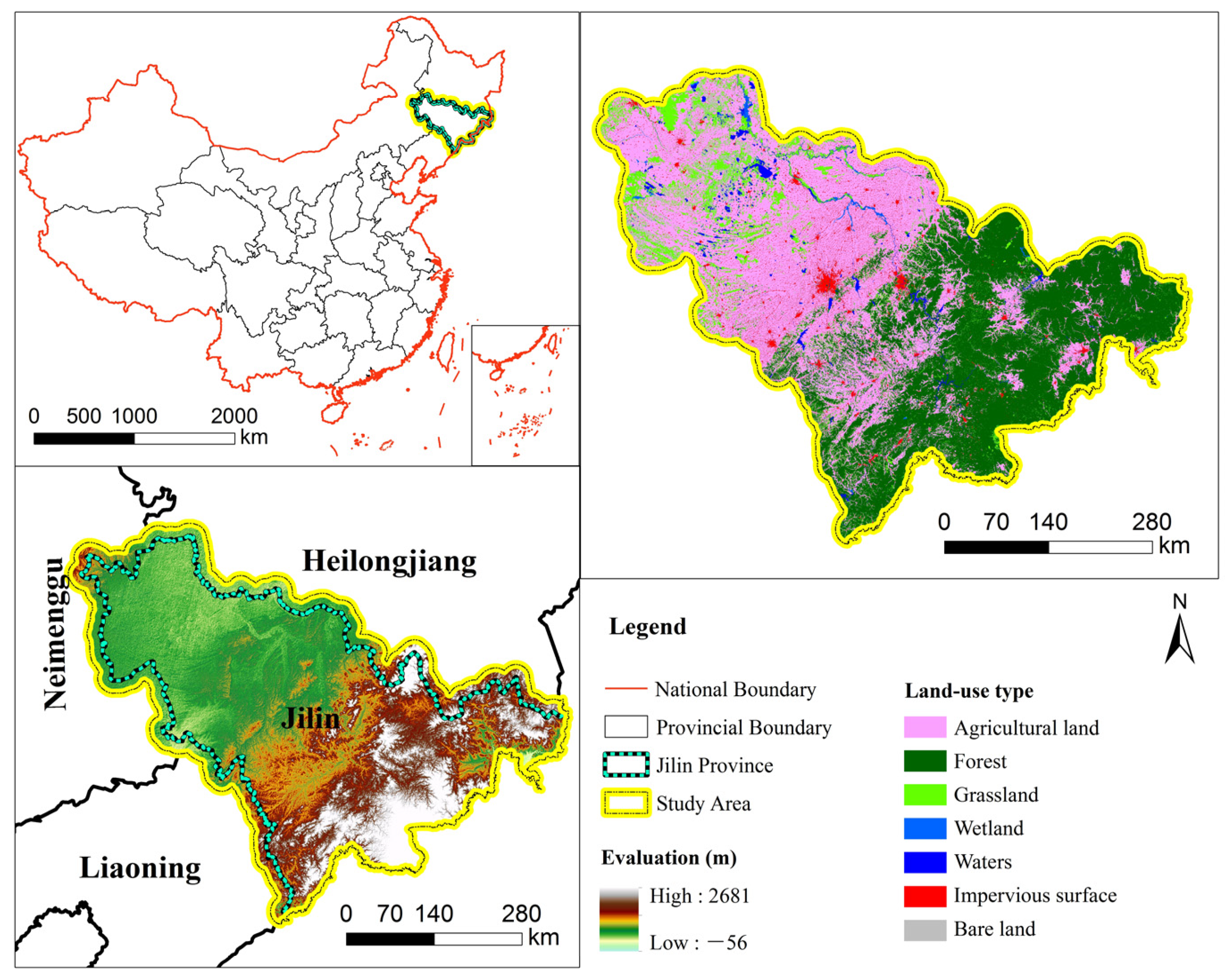
2. Study Area

Jilin Province (121°38′–131°19′ E, 40°50′–46°19′ N) (Figure 1) is nestled in the heart of Northeast China, bordering Liaoning Province to the south, the Inner Mongolia Autonomous Region to the west, and Heilongjiang Province to the north. It governs eight prefecture-level cities and one autonomous prefecture, encompassing 60 districts and counties. With a total population of 24.0735 million in 2020, the eastern, central, and western regions account for 19.80%, 56.86%, and 23.34% of the population, respectively. Jilin Province boasts a wealth of ecological resources; the Changbai Mountains in the east serve as a vital ecological shield in Northeast China, with water conservation among its functions. The central plain is a significant grain-producing area, while the grassland wetland ecosystem in the west features a unique distribution and functions. This diverse, multifunctional, and zonal terrestrial ecosystem is representative of the nation, playing an irreplaceable role in the national ecological security strategy. The province is home to nationally protected wildlife and plants, such as the Siberian tiger, the Amur leopard, the eastern white stork, the Northeast Yew, and the long white pine. Forests, grasslands, wetlands, and other natural resources offer ecological services like soil and water conservation, as well as landscape recreation, and support industries like logging, livestock production, and fisheries.

These resources provide the material basis and act as the spatial carrier of the province’s economic and social development and ecological civilization construction. However, Jilin Province still grapples with systemic ecological issues, including severe soil erosion, mounting pressure on biodiversity protection, and desertification and salinization trends in the west, which remain uncontrolled at their core. To systematically identify key areas for protection and restoration within the province’s “social–ecological” system, targeted measures in regional development are essential. Establishing a social–ecological security pattern aids in comprehensively understanding the socioeconomic and ecological development patterns of Jilin Province, pinpointing crucial zones for protection and restoration, and understanding the mismatch between the province’s socioeconomic development and ecological system services. This pattern also provides a scientific basis for advancing green and low-carbon economies, optimizing the natural ecological environment, and enhancing ecosystem services in Jilin Province. Considering the fluidity and extraterritorial effects of ecosystem services [10], and referring to relevant studies [22], a 20 km buffer zone surrounding Jilin Province was included in the research.

3. Materials and Methods

Liu Jianguo et al. from Michigan State University have systematically elucidated the concept of coupled human and natural systems (CHANS). They posit that CHANS encapsulate the intricate web of interactions between human activities and natural elements. The research within this domain zeroes in on the patterns and processes within “social–ecological” systems, examining the dynamics and feedback loops that characterize these interactions. It also delves into the intra-scale and cross-scale dynamics among the various elements within the system [23]. Within the framework of CHANS, the coupled “social–ecological” system is envisioned as a complex hierarchy of entities that interact at multiple levels of organization. These interactions form a dense network, creating a tapestry of interwoven relationships [2]. To unravel the complexity of this interplay between societal and ecological realms, ecosystem services serve as a pivotal entry point. Ecosystems and their ecological processes are the wellspring of ecosystem services, which are then harnessed by the social system to foster the ecological well-being of human societies. This constitutes a comprehensive mechanism for the demand and supply of ecosystem services [24]. A thorough analysis of the social-landscape ecological security pattern, predicated on the effect on demand and supply of ecosystem services, enables a profound analysis of this multifaceted dual system (Figure 2).

3.1. Data Sources and Preprocessing

Multi-source datasets, including land cover datasets, physical geographic datasets, socioeconomic datasets, and other auxiliary datasets for 2020, were applied in order to evaluate ecosystem services in this study (Table 1). In the preprocessing stage, all data were uniformly converted into the GCS_WGS_1984 coordinate system and UTM projection, and a 1 km × 1 km resolution was generated after resampling.

3.2. Research Methods

3.2.1. Ecosystem Service Supply

Ecosystem service supply is defined by the competence of an ecosystem to offer matter and products that are anticipated by human society in a sustainable manner within a specified geographical area [25].

Based on certain production functions and empirical modeling methods, the InVEST model establishes a specific ecological process equation model, which can display the supply situation of ecosystem services to users in spatial patterns such as maps. The model can fully incorporate supply situation of ecosystem services into research system for scholars to conduct relevant research [16]. The procedure for calculating ecosystem service supply is detailed in the Appendix A.

After normalizing the data for each ecosystem service supply, the results are aggregated using the same set of weights. This approach can help obtain a comprehensive overview of the ecosystem services supply in Jilin Province.

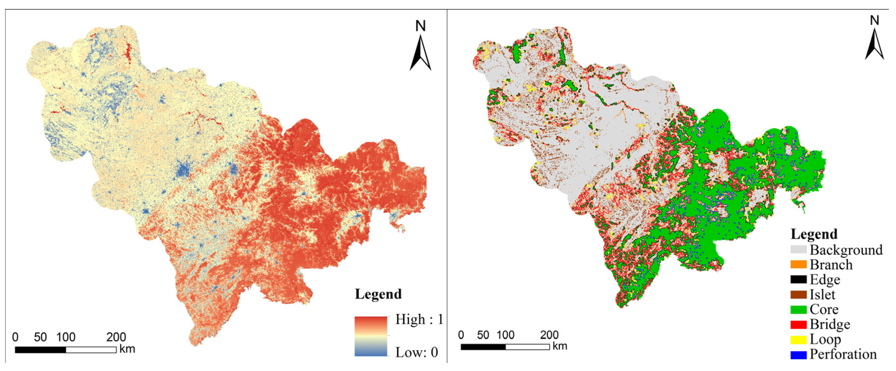
3.2.2. Ecological Source Determination—MSPA

Morphological spatial pattern analysis (MSPA) measures and segments grids on the basis of the principle of mathematical morphology; it emphasizes structural connectivity in spatial form and ecological processes and ecological networks in principle to enhance the scientificity of ecological source selection [17,18].

To conduct the MSPA, the categories of land that were taken as the foreground were forestland, grassland, wetland and water areas. The remaining land types were assigned to the background. After they were converted into GeoTIFF binary maps, distinct landscape types, namely the bridge, loop, core, islet, edge, perforation, and branch, were discerned via Guidos 3.3 software. Core patches were selected as ecological source areas, and patches that were too small (less than 1 km²) to provide favorable conditions for species survival and dispersal were removed. By using Conefor 2.6 software, the probability of connectivity (PC) [26,27] and integral index of connectivity (IIC) [28,29] were calculated on the basis of the topological space. The patch importance index was calculated through the summation of them with equal weighting applied to each.

d_{I I C} = \frac{\sum_{i = 1}^{n} \sum_{j = 1}^{n} \frac{A_{i} \times A_{j}}{1 + C_{i j}}}{{A_{e}}^{2}}

d_{P C} = \frac{\sum_{i = 1}^{n} \sum_{j = 1}^{n} A_{i} \times A_{j} \times {P_{i j}}^{*}}{{A_{e}}^{2}}

d = {0.5 d}_{I I C} + {0.5 d}_{P C}

where

d_{I I C}

is the overall connectivity index,

d_{P C}

is the possible connectivity index, d is the importance index of patches, A_e represents the total area, n represents the total number of patches in the landscape surface e, A_j and A_i are the areas of patches j and i, and C_ij is the total number of connections between patches j and i under the shortest path. P_ij is the maximum connectivity probability between patches j and i. Finally, patches with a high importance index (top 25%) were deemed to be ecological sources of MSPA.

3.2.3. Demand for Ecosystem Services

The demand for ecosystem services can be defined as quantity that is presently used, depleted, or expected to be obtained from all services and products provided by ecosystems, as well as the preferred demand of human society in a particular region [25], which depends mainly on the level of socioeconomic development [30]. Xie Gaodi et al. believed that the three levels of material, safety, and spiritual needs are the main aspects of human needs [31]. Wu Xuan et al. divided human demand for ecosystem into material culture, ecological security, and environmental quality [32]. Referring to the classification methods published by scholars, this paper proposes a classification of ecosystem service demand based on three groups: primary, development, and advanced demand. The ecosystem service demand indicators correspond to the supply indicators to facilitate supply and demand comparison and status quo analysis. Among them, primary demand is the essential basic condition furnished by the ecosystem, without which human survivability in modern society would be unfeasible; development demand is selected from the perspective of industrial production and other economic and social development; and advanced demand refers to the diversified spiritual needs such as leisure tourism for people with leisure time and discretionary economic income.

Primary demand pertains to fulfilling the fundamental survival requirements of humans. Population density most directly drives the escalation in the demand for ecosystem services. Consequently, indicators tied to essential human needs—such as respiration, potable water, and food production—were categorized under primary demand (Table 2).

The per capita GDP, fixed asset investment, per capita electricity consumption, night light intensity, construction land density, and road network density are important indicators used to measure regional development, reflecting the development intensity of human activities. The density of secondary industry, demand for industrial water resources, carbon and oxygen emissions, discharge of wastewater and waste, and degree of air pollution serve to reflect how human productive actions impact the ecosystem, both in terms of inputs and outputs. These factors were classified as development demand.

The advancement of tertiary industry is an inevitable result of improvements in productivity and social progress. The growth in retail sales of consumer goods is indicative of an improvement in living standards, both material and cultural, as well as an increase in the purchasing capacity of social goods and the level of activity within the retail market. The growth of tourism facilities, tourism places, and the number of tourists reflects people’s increasing spiritual demand for a better ecological environment via a material basis, which was classified as advanced demand.

3.2.4. Circuit Theory

The circuit theory in landscape ecology is to compare material flow or gene flow to electric current and define the resistance of their migration and diffusion as resistance surfaces. The movement of current (material flow or gene flow) in the circuit (path between sources) is disturbed by the resistance (resistance surface). The current in the region with lower resistance moves more smoothly, and the greater the cumulative current value in a region, the more optimal the circuit network connectivity. According to the characteristics of random walk of current (material flow or gene flow) in the circuit, diverse calculative methodologies are applied in order to evaluate the performance of multiple scattered paths in the network [33,34]. The field of circuit theory has been employed in the analysis of network connectivity across a range of disciplines, including ecology, chemistry, neuroscience, economics, and sociology [35]. Therefore, it is also applicable in the research of this paper.

3.2.5. Construction of Landscape Ecological Security Pattern

(1) Supply sources. Various ecosystem supply services reflect their functional attributes, whereas MSPA measures interregional structural connectivity in accordance with the spatial form attributes. Therefore, the overlapping patches of the high-level integrated supply area of ecosystem services (top 25%) and the ecological source area of MSPA were taken as the final supply source. Then, the importance of the supply source was categorized within three levels utilizing the Natural Breaks Method (slightly important, generally important, and extremely important). The calculation process is outlined in the following formula:

I_{es} = 0.5 d + 0.5 m

In the formula, I_es is the importance score of the supply source, d is the patch importance index, and m is the average value of comprehensive supply services.

(2) Landscape comprehensive resistance surface. The movement of energy and matter between ecological sources is subject to the effects of multiple elements, including actions of humanity and geographical background [36]. Land use type exerts a significant influence on the movement of ecological flow, so it was used as a resistance factor, and the resistance coefficient was set with reference to relevant studies [37]: forestland 1, wetland 10, grassland 50, water 100, agricultural land 200, bare land 500, and impervious surface 1000. The effect resulting from human actions was manifested in ecosystem service demand, and landscape resistance surface was modified accordingly. The stronger the demand is, the greater the interference and obstruction effect and the higher the resistance value. Through this approach, the landscape comprehensive resistance surface was obtained. The calculation formula is as follows:

R_{e} = R_{v} \times \frac{E S D_{i}}{E S D_{l}}

where R_e is modified landscape comprehensive resistance value, R_v is land use resistance value, ESD_i is the ecosystem service demand value, and ESD_l represents average ecosystem demand value for land type to which the raster corresponds.

(3) Ecological corridor. In accordance with the principles of circuit theory, the linkage mapper module, as incorporated within the Circuitscape plug-in of ArcGIS 10.8 software, was employed for the purpose of identifying the ecological corridor within the designated study area. The following formula is utilized for calculation:

I = \frac{U}{R}

where I represents connected ecological flow between source areas, U represents the connected probability of source areas, R represents resistance of ecological flow.

Subsequently, the Centrality Mapper tool was adopted for calculation of flow centrality and classification of the degree of significance attributed to the ecological corridors, in accordance with the Natural Breaks Method. (slightly important, generally important, and extremely important).

(4) Ecological nodes. The ecological nodes are constituted by pinch points and barrier points, which were calculated by pinch point mapper and barrier mapper modules in the Circuitscape plug-in of ArcGIS software, respectively.

3.2.6. Construction of a Social–Ecological Security Pattern

(1) Demand source. After the normalization of each ecosystem service demand in the study area, the entropy method and analytic hierarchy process were used to combine objective and subjective weights, and the two weights were averaged to obtain the final weight coefficient. The comprehensive demand value of the ecosystem was obtained by superimposing the weight coefficients, and the patches with an area exceeding the minimum threshold (1 km²) in the high-value area (top 25%) were extracted as the demand source. Then, the importance levels of the demand source were classified (extremely important, generally important, and slightly important) in accordance with the Natural Breaks Method through the comprehensive demand value of the ecosystem.

(2) Social–ecological resistance surfaces. The mismatch and imbalance of ecosystem service demand and supply lead humans to actively approach areas with high levels in terms of ecosystem service provision close to their spatial range, with the aim of achieving ecological well-being. In this process, the level of spatial reachability determines the strength of the hindrance when humans acquire ecological material, energy, and information flow. Therefore, spatial reachability was calculated via the Gaussian two-step floating catchment area method as resistance surface. The following formula is used for the calculation [38]:

R_{j} = \frac{S_{j}}{\sum_{k \in d_{k j} \leq d_{0}} D_{k} G (d_{k j})}

where R_j is the supply-demand ratio of supply source j, S_j is the area of supply source j, d_kj is the cost distance from supply source j to demand source k, d₀ is the distance threshold, D_k is the population of demand source k within the search domain of supply source j with radius d₀, and G (d_kj) is the Gaussian attenuation function.

G (d_{k j}) = \frac{e^{- \frac{1}{2} \times {(\frac{d_{k j}}{d_{0}})}^{2}} - e^{- \frac{1}{2}}}{1 - e^{- \frac{1}{2}}} (d_{k j} \leq d_{0})

A_{i} = \sum_{l \in \{d_{i l} \leq d_{0}\}} R_{l} G (d_{k j})

where A_i is the spatial accessibility of demand source i to the ecological supply source, d_il is the cost distance from demand source i to supply source l, and R_l is the supply-demand ratio of supply source l within demand source i.

In the “social–ecological” system, the ecological flow also naturally flows from supply source to demand source due to homeopathic differences [39,40]. Therefore, this natural flow trend of the ecosystem service supply should also be incorporated within establishment of social–ecological resistance surface as a correction factor, and the spatial accessibility resistance value should be corrected through the reciprocal value of ecosystem service supply [41]. The specific calculation is represented by the following equation:

R_{c} = \frac{E S S_{i}}{E S S_{l}} \times A_{i r}

R_c is the revised social–ecological resistance value, ESS_i is the reciprocal value of ecosystem service supply, ESS_l is the reciprocal value of average ecosystem service supply of grid corresponding to the land class, and Air is the spatial accessibility resistance value.

(3) Supply–demand corridor. Supply–demand corridors are channels of material and energy transfer between human society and natural ecosystems. In accordance with supply source, demand source, and social–ecological resistance surface, the supply–demand corridor was constructed via circuit theory, in the same method as the construction of ecological corridors. The Centrality Mapper tool was then adopted for calculation of flow centrality and classification of the degree of significance attributed to the supply–demand corridor in accordance with the Natural Breaks Method (extremely important, generally important, and slightly important).

3.2.7. Ecological Network Integrity Evaluation

The ecological network integrity method was adopted for the purpose of evaluating the overall situation of the ecological network, and assessment criteria comprise the following elements: network circuitry (α), network connectivity (γ) and line-to-node ratio (β). Prior to and following the proposed optimization of the social–ecological security pattern, a comparative analysis of its integrity was conducted [42,43,44]. The detailed calculation procedure is shown in the Appendix A.

4. Results

4.1. Ecosystem Service Supply

The distribution of ecosystem service supply exhibits a spatially varying pattern, with a higher level of supply observed in the eastern regions and a lower level in the western regions of Jilin Province. Areas exhibiting low levels of supply are predominantly located at the center of Baicheng City, the south of Changchun City, the south of Siping City, and the west of Jilin City. The regions with high levels of supply are situated in Yanbian Korean Autonomous Prefecture, Tonghua City, and Baishan City, due to the significant ecosystem services provided by woodlands and grasslands, which include carbon fixation and oxygen release, soil conservation, habitat quality, and water conservation. A comparison of the area of high-value of importance index with the range of high-value of ecosystem service supply revealed an overlap of 90.47% (Figure 3 and Figure 4).

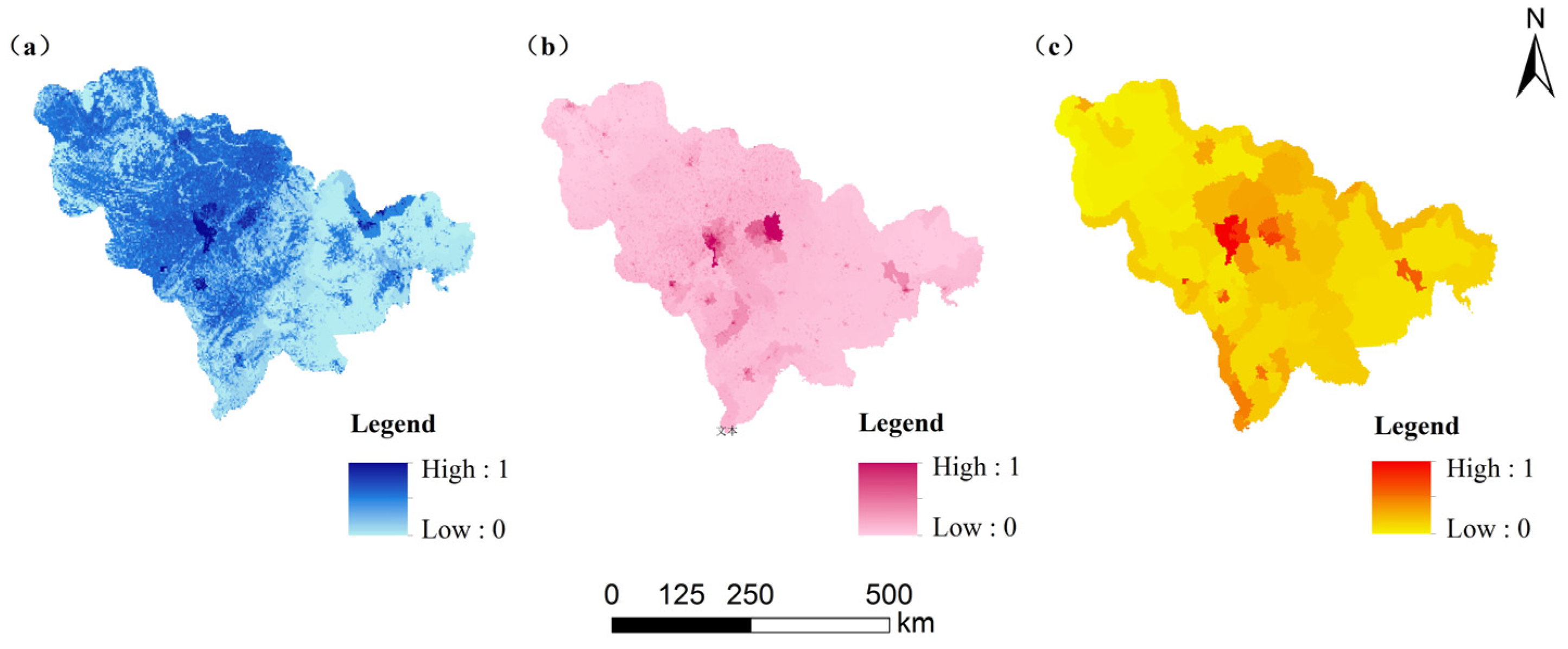
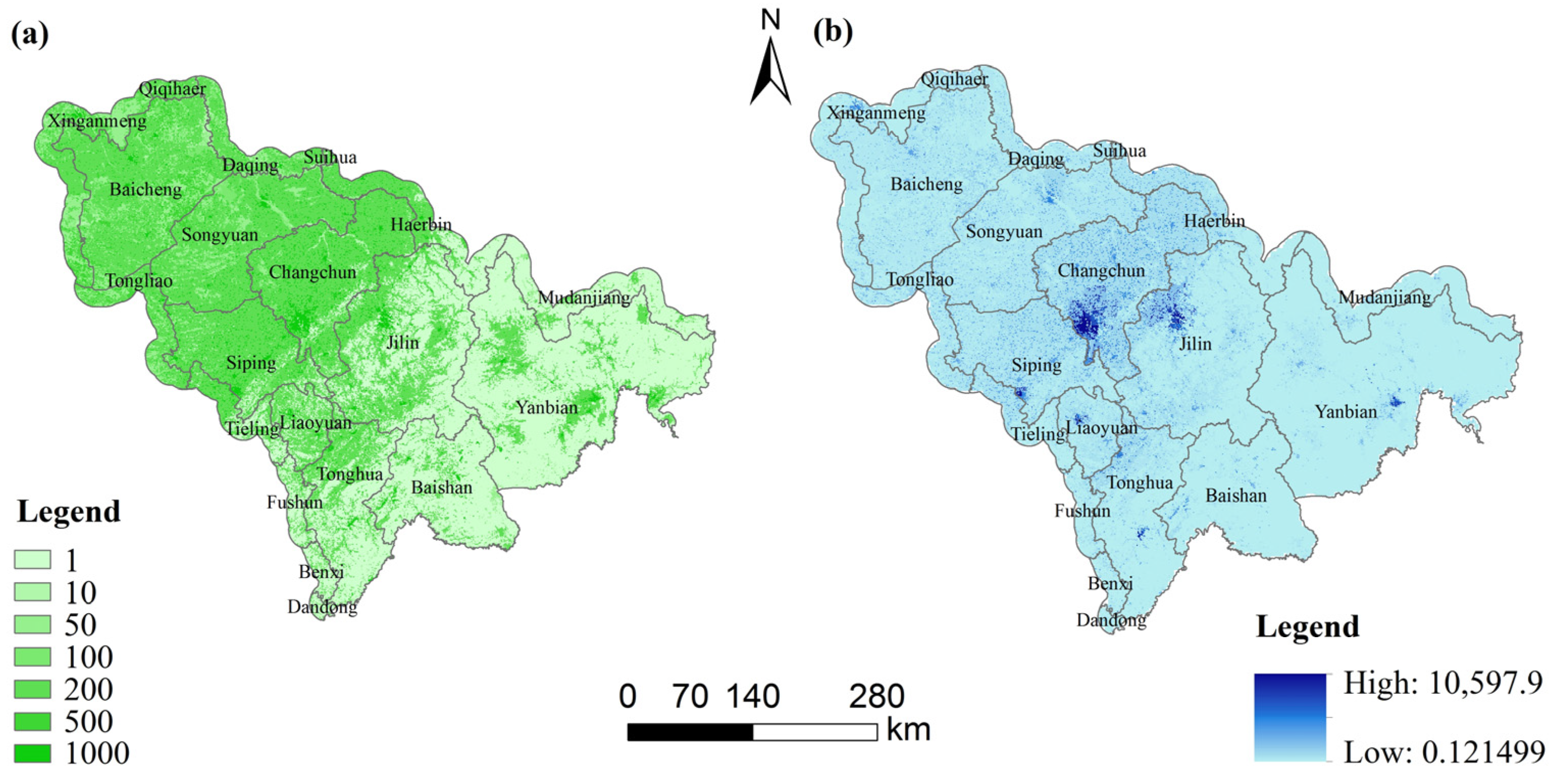
4.2. Ecosystem Service Demand

The demand for ecosystem services in Jilin Province is notably higher in the central areas compared to the eastern and western regions. High-demand zones are predominantly found in the southern parts of Changchun city, the western areas of Jilin city, the northern sections of Songyuan city, the southern regions of Siping city, the central areas of Liaoyuan city, the middle parts of Tonghua city, and the central areas of Yanbian Korean Autonomous Prefecture. These high-demand areas share common traits such as dense population, advanced industry, and a significant level of development. It is apparent that there is a clear imbalance between the supply and demand of ecosystem services in these regions (Figure 5 and Figure 6).

4.3. Ecological Security Pattern

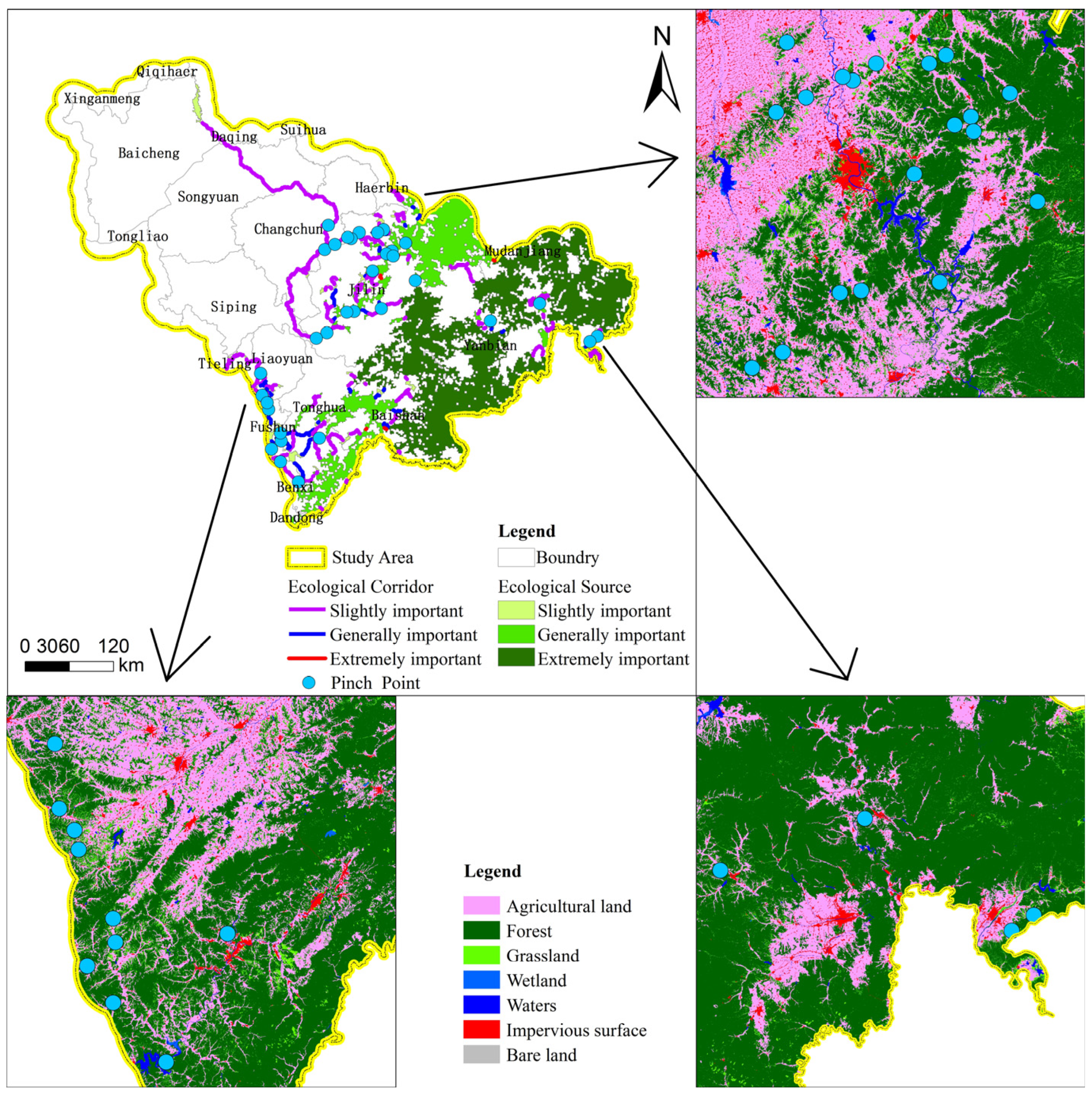
4.3.1. Landscape Ecological Security Pattern

(1) Supply source. The whole number of 101 supply sources were discerned, encompassing an area of 54,393.02 km², representing 23.05% of the study region. Within this area, forestland constituted the predominant land cover type, constituting 95.04% of the area, followed by grassland (3.95%), water area (0.67%), and wetland (0.34%). With regard to the spatial distribution, the supply source east of the study area was large and densely distributed, composed mainly of woodland and grassland, and near Huashan National Forest Park, Changbai Mountain National Nature Reserve, the Tumen River, and other places. In the middle, the supply source area was small and scattered, composed mainly of woodland and water, and was mainly distributed near the Shitoumen Reservoir, Songhua Lake, Yantongshan, and other places. There was only one supply source in the northwest, which was mainly wetland, grassland, and water, and it was located in Momoge National Nature Reserve (Figure 7).

Among the supply sources, two extremely important supply sources, representing 67.09% of the overall area, were located within the range of Baishan city and Yanbian Korean Autonomous Prefecture. Forty-six generally important supply sources, accounting for 29.18%, were located in Jilin city, south of Tonghua city, and west of Baishan city. There were 53 slightly important supply sources, accounting for 3.73%, scattered in the eastern portion of the study area.

(2) Resistance surface. The comprehensive landscape resistance surface, obtained from the land use type resistance value modified by the total ecosystem service demand, displayed a progressively declining distribution pattern from the center to the periphery. The central area of high resistance value was predominantly situated within the Jilin City northwestern and Changchun City southern areas, which had high ecosystem service demand and high human interference intensity; these factors were not conducive to overall ecosystem connectivity. The adjacent region surrounding the high-value region also substantially obstructed the flow of matter and energy (Figure 8).

(3) Corridors and nodes. On the basis of circuit theory, the research region was found to comprise 166 ecological corridors, collectively extending 3157.58 km in length. Among these corridors, the one linking the Jingyuetan National Forest Park in the center to the Momoge National Nature Reserve in the northwest was identified as the longest, while the remaining corridors were located in the middle, eastern, and southern regions, exhibiting varying lengths (Figure 7).

Among them, the length of 12 extremely important ecological corridors accounted for 1.66%. These corridors were distributed mainly in Jilin city and Baishan city. Thirty-eight generally important ecological corridors accounted for 15.16% of the total length. Finally, 116 ecological corridors of slight importance accounted for 83.18%.

According to circuit theory, there were 33 ecological pinch points, with the majority situated at intersection points or important turning points of ecological corridors. The distribution was concentrated in the middle and south and scattered in the east, among which five ecological pinch points were densely distributed on the ecological corridor connecting the Shitoumen Reservoir and Shulan Forest Park. The ecological pinch points were primarily agricultural land, forestland, and water areas, with an average resistance value of 14.29. This indicates that the pinch points are of critical importance for maintaining the structural integrity of the ecosystem, serving as vital hubs for the exchange of energy and substance with minimal disruption (Figure 9).

There were 18 ecological barrier points (i.e., high-value areas of cumulative current recovery), most of which were concentrated in the central region, while a few were situated in the eastern portion of research area. Among them, five ecological barrier points were densely distributed on the ecological corridor which connects Momoge source area and Jingyuetan source area. The land type was principally constituted by imperious surface and cultivated land, with an average resistance value of 1817.16, which seriously hinders species migration and diffusion and information exchange, leading to ecological circulation obstruction and damage to ecological function. Ecological restoration should be prioritized, ecological barrier points should be restored, and an ecological security pattern with efficient connectivity and good habitat should be built (Figure 10).

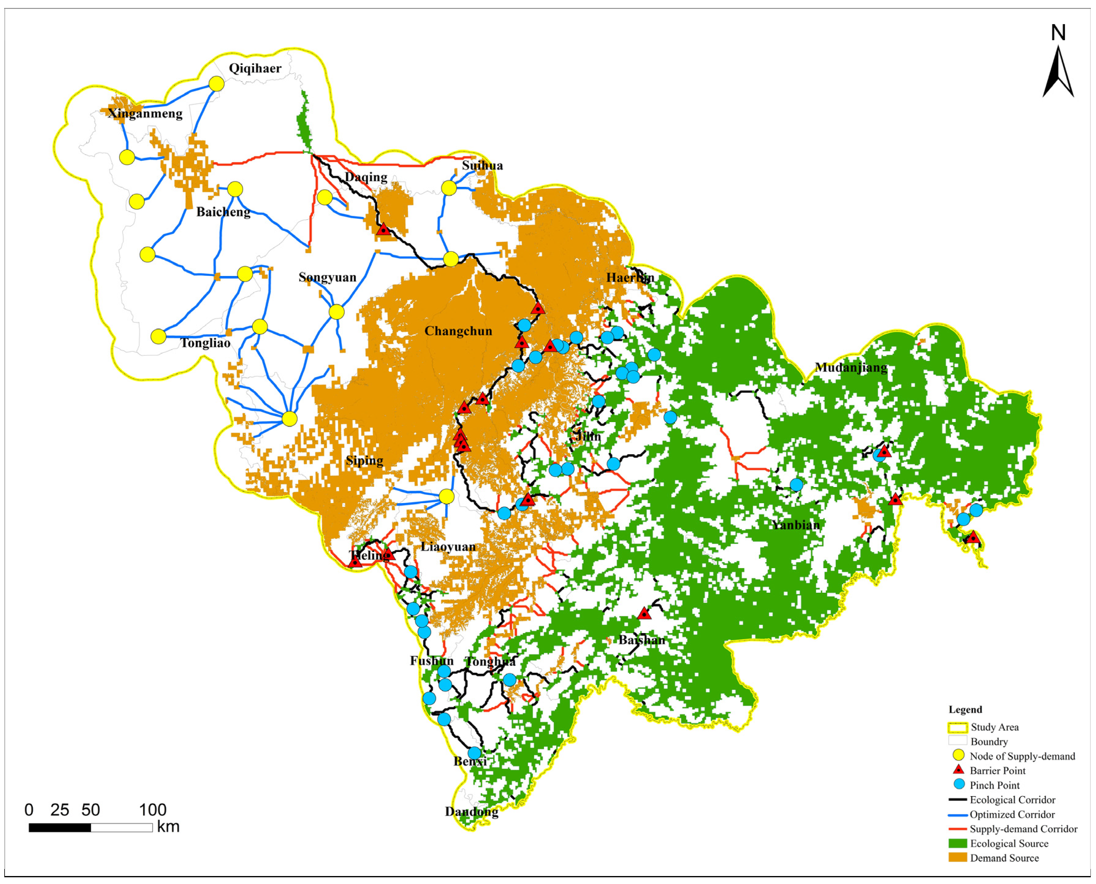
4.3.2. Social–Ecological Security Pattern

(1) Demand Source. The whole number of 119 demand sources were discerned, encompassing an area of 44,904.98 km², representing 19.03% of the study area. In further analysis, it was determined that 86.89% of this area was classified as agricultural land, 13.06% as construction land, and 5.00% as unused land. In consideration of spatial distribution of demand, the area of demand source in the central portion was large and densely concentrated within the research area, comprising 87.89% of Changchun city and 51.31% of the area of Siping city. The areas of demand sources in the eastern and western regions were small and scattered across various cities, and the land types were largely comprising impervious surface and agricultural land.

Among them, 11 extremely important demand sources, accounting for 58.82%, were located mainly in southern Changchun city, the middle of Siping city and Ningjiang District of Songyuan city. A total of 60 generally important demand sources, representing 40.42% of the entire region, were identified, with the majority situated in Jilin City, the Baicheng Taobei District, northern Changchun City, and northern Tonghua City. A total of 48 slightly important demand sources, constituting 0.76% of the overall region, were dispersed throughout Tonghua City, Songyuan City, and Baicheng City.

(2) Resistance surface. The spatial accessibility resistance surface obtained via the Gaussian two-step floating catchment area method took the central urban areas of Changchun city, Baicheng city, and Liaoyuan city as the low-value areas. In these regions, as peripheral accessibility gradually decreased, the resistance value increased progressively. This phenomenon can be attributed to the substantial influence of the road network on accessibility [45], with the central urban zone exhibiting a higher density of road networks, consequently enhancing accessibility. The spatial accessibility resistance surface was modified by the flow trend of the ecosystem service flow, thereby reflecting the spatial disparities inherent to the accessibility of disparate ecosystem service supplies. The obtained social–ecological resistance surface distribution was relatively scattered, with the overall resistance value being smaller in the east and greater in the west. The resistance value of central urban areas still tended to increase from the center outward approximately (Figure 11).

(3) Corridor. In accordance with the principle of circuit theory, a total of 150 supply–demand corridors, encompassing a combined length of 1565.60 km, were determined through the construction of a “supply source—demand source—social–ecological resistance surface” within the designated research area. The five supply–demand corridors connecting the Momog supply source and its surrounding demand sources in the northwest are relatively long, while the remainder are dispersed throughout the central, eastern, and southern areas, exhibiting a range of lengths. The overall distribution of supply–demand corridors was uneven, and the western demand area lacked supply–demand corridors to connect with the supply area. The addition of supply–demand nodes is urgently imperative to satisfy the requirements of various ecosystem services in the demand area, guarantee natural connectivity and uninterrupted flow of energy and material, as well as to improve overall ecological connectivity of the research region (Figure 12).

Nineteen extremely important supply–demand corridors, representing a combined length of 3.01%, were predominantly situated within Jilin City and Liuhe County of Tonghua City. There were 31 generally supply–demand corridors, representing 6.72% of the entire length, that were primarily situated in Jilin City, Tonghua City, and Dongfeng County of Liaoyuan City. There were 100 slightly important supply–demand corridors, representing 90.27% of the entire length, that were scattered throughout the study area.

4.4. Optimization of Social–Ecological System Patterns

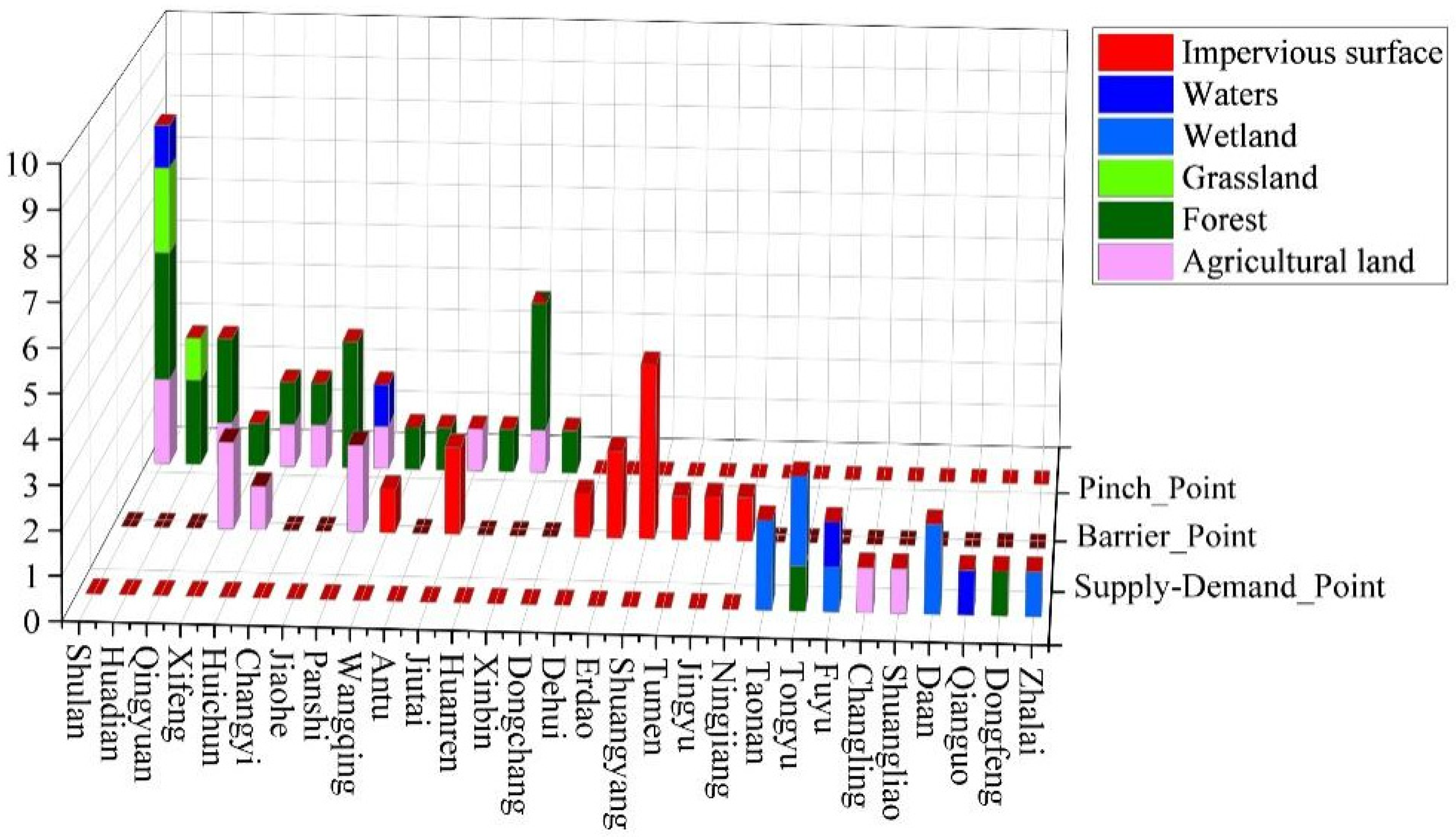
4.4.1. Additional Supply–Demand Nodes

As it is difficult to coordinate the development of social and economic structures with the natural ecological surroundings in some regions, the supply of ecosystem services has difficulty meeting human needs. The addition of ecological supply–demand nodes is urgently needed to improve human ecological well-being, enhance the integrity and resilience of the “social–ecological” system, and achieve regionally coordinated progression.

In order to ensure that each demand source can find the supply source nearby to provide ecosystem services for it, the high-value area of ecosystem service supply capacity that is the closest to the isolated demand source and has been removed due to its small area (less than 1 km²) is taken as the supply–demand node, so as to form a structural connection with the isolated demand source and optimize the social–ecological network. These added supply–demand nodes are all high-value areas obtained from the comprehensive results of various ecosystem service supply calculated by the research method stated in this paper before, and they are also high-value patches of importance index obtained after MSPA. A series of ecological restoration programs can serve to achieve the purpose of making the area of the added supply–demand nodes larger and the supply ability of ecosystem services stronger. According to existing ecological security pattern, 14 supply–demand nodes are added (Figure 13) to avoid the fragmentation of ecosystem integrity and connectivity and prevent the fragmentation of ecological space. These nodes are distributed mainly in Baicheng city and Songyuan city in the western part of research region and included Xianghai Lake, Chagan Lake, Tumuji, and other national nature reserves. Most of the supply–demand nodes are areas with high supply and service values below the minimum area threshold and are mainly wetlands, water areas, and forestlands.

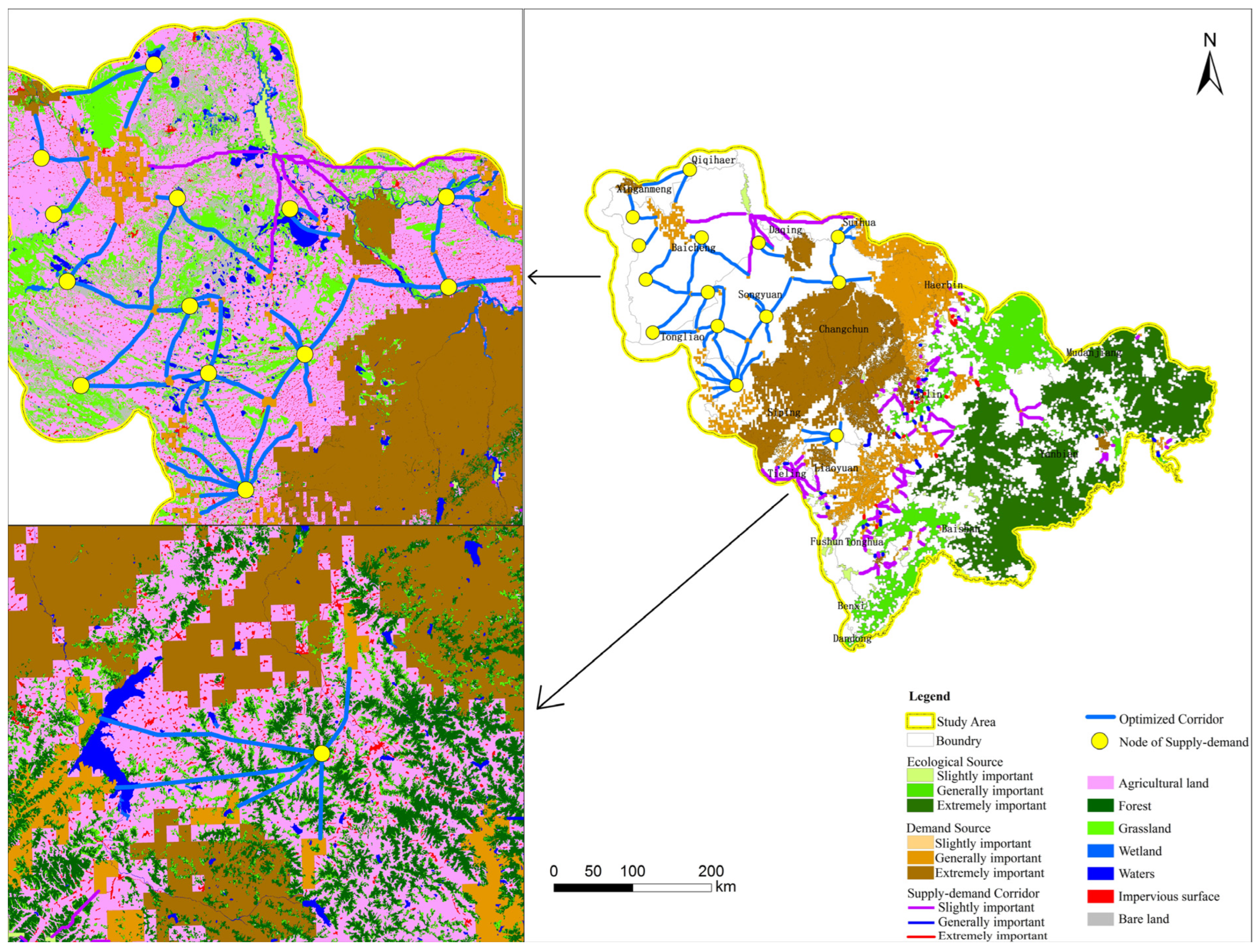
4.4.2. Optimize Corridor Connections

In order to detect the optimal corridor, the circuit theory approach was utilized, integrating the additional supply–demand nodes, the original supply source, demand source and social–ecological resistance surface. The newly added corridor connecting the supply–demand nodes and the isolated demand source in the identification result is the optimized corridor. A more balanced layout, more reasonable structure and stronger function of Jilin Province’s social–ecological security pattern was constructed, which was founded upon “supply and demand source—social–ecological resistance surface—supply–demand corridor” and supplemented by “supply–demand node—optimization corridor”.

On the basis of the additional supply–demand nodes, 47 optimized corridors with a cumulative length of 1773.78 km were constructed to connect the source of demand for ecosystem service supply, which was difficult to obtain in the western and central sections of the research region. The additional supply–demand nodes and optimized corridors were distributed uniformly in the western section of the research region and thus enhanced the connectivity between patches and improved the multifunctional ecological network of the “source corridor network and habitat connectivity.” The results of the ecological network integrity evaluation revealed that the α index increased from 0.39 to 0.56, the β index increased from 1.74 to 2.07, and the γ index increased from 0.59 to 0.71, indicating that the degree of closure, connection level, and ecological efficiency of the optimized social–ecological network in the research region were significantly enhanced and that there were more paths for humans to achieve ecological well-being. The circulation of information, material, and energy was better, consolidating the social–ecological security support system (Figure 13).

5. Discussion

5.1. Zone Protection and Restoration Suggestions

Considering the spatial distribution characteristics of “sources-corridors-nodes”, the eastern part of Jilin Province, renowned for its robust ecosystem foundation and elevated social–ecological well-being, has been designated as a core protected area. The strategic approach prioritizing natural restoration, complemented by artificial measures, has been implemented. In contrast, the central area of Jilin Province, characterized by high social–ecological demands and challenges in obtaining ecological benefits, was divided into ecological demand zones. Conversely, the western region of Jilin Province, with poor ecosystem service function and severe damage to the integrity of the “social–ecological” system, was designated as a core restoration area, and the corresponding restoration strategy of “artificial restoration is the primary one and natural restoration is the secondary one” was adopted. The specific suggestions for each zone are as follows:

(1) Many ecological supply sources, ecological corridors, and supply–demand corridors are concentrated in the eastern core protected area. In the Changbai Mountain Global Geopark, the area should strengthen the construction of key national ecological functional areas and constantly enrich the “ecological museum” and “species gene bank”. On the premise of not disturbing the social landscape ecological security pattern, the planning and guidance of human beings should actively obtain ecological welfare, ecological value, economic benefits, and appropriate development of the forest tourism health industry to meet human needs and ensure the dual goals of ecological security. Moreover, as the main provider of ecosystem services, the establishment of a compensatory mechanism on a cross-regional transverse basis for ecosystem services is a viable proposition [11,46]. The barrier points and pinch points in the east are scattered in northern Antu County, southern Wangqing County, middle Tumen city, and southern Hunchun city. The pinch points are largely forestland and cultivated land, and the barrier points are construction land. The ecological pinch points are densely located at the south, running from north to south through Liaoyuan city, Tonghua city, and the junction of Liaoning Province, involving cross-provincial ecosystem information exchange and energy flow. More attention should be given to the construction of their connectivity, cross-provincial cooperation, and overall planning of protection measures to avoid or reduce the negative human interference that may be caused by ecological pinch points (Figure 14).

(2) The central ecological demand area is a concentrated distribution area of ecological demand sources, ecological corridors, supply–demand corridors, barrier points, and pinch points. As the driving force for revitalization of Jilin province, this region is experiencing a significant deficit in ecological space, largely due to its considerable population concentration and advanced level of industrialization. This has led to a number of pressing issues pertaining to the population, resources, and the environment. In the region, Shulan City exhibits the highest concentration of ecological pinch points (8), while the Shuangyang District displays the greatest density of ecological barrier points (4) (Figure 15). However, the ecological supply sources are very scarce, and it is difficult to meet regional human ecological needs. While regional ecological construction continues to increase, the ecosystem service function can be comprehensively improved by adding ecological supply–demand nodes and optimizing corridors near Erlong Lake Scenic spot at the junction of Yitong Manchu Autonomous County and Dongfeng County. The farmland in the middle of the region is known as the “golden corn belt” and the “township of black land”. As the core area of national grain production, the focus should extend beyond mere land and production technology to encompass the ecological environment in which food is produced. Through measures such as clearing and returning forestland, the multiple functions of protecting black land and conserving water sources can be considered, effectively improving the agricultural ecological environment and building a strong ecological protection barrier. To ensure food security, more attention should be given to landscape versatility in rural areas, and tourism products and services should be created on the basis of the traditional resources of local agricultural landscapes as one way to achieve ecological well-being [47]. We should continue to optimize ecological protection and restoration work, build a functional social–ecological pattern, increase the carrying capacity of social development, create green wealth and welfare, accelerate economic and social transformation and upgrading, promote a prosperous ecological culture, and foster the ecological core value of a community of life for man and nature.

(3) In recent years, in Western Jilin, a typical ecologically fragile region in China, soil desertification, expansion of saline alkali land, grassland degradation, and wetland water shortages have become increasingly serious [48]. Among the core restoration areas in the west, the larger demand sources are distributed mainly in Taobei District of Baicheng city, the northern part of Qiangueros Mongolian Autonomous County of Songyuan city, and Ningjiang District of Songyuan city, whereas the other smaller demand sources are scattered throughout the region. At present, there is only one ecological supply source near the Momoge National Nature Reserve in the region, and the discrepancy between the ecological demand and supply is relatively serious. The grassland ecosystem has been degraded to different degrees, the wetland has shrunk, the aquatic environment has deteriorated, and the ecological environment is relatively vulnerable; thus, an effective ecological restoration process urgently needs to be accelerated. Ecological protection and restoration in the region ought to prioritize restoration by restoring the functions of grasslands and wetlands, promoting the control actions for land desertification and salinization, curbing the trend of desertification, strengthening weak links in the ecosystem, and building a more dynamic ecological economic zone in the western region. Therefore, we should focus on adding supply–demand nodes with relatively strong ecological supply capacity and optimization corridors with relatively small resistance, among which Tongyu County of Baicheng city has the most supply–demand nodes (3) (Figure 15). Artificial intervention procedures warrant consideration as a means of optimizing ecosystem service functions of supply–demand nodes. Such measures include comprehensive management of desertified land in Tongyu County, where sand dunes cover a wide area; increases in vegetation coverage; and the construction of supporting infrastructure to promote vegetation restoration. In Chagan Lake and other areas where freeze-thaw damage is serious, steep slopes, rivers, and lake shorelines should be treated, and a lakeside buffer zone should be built to reduce the amount of pollutants entering the lake. The protection and restoration of wetlands in Xianghai National Nature Reserve and Zhenlai Huancheng National Wetland Park should constantly be strengthened to optimize the ecological functionality of these wetland ecosystems. The construction of green infrastructure in regions that are not served by ecological supply sources continues to be a priority; the existing ecological supply sources should be supplemented, and the interconnection of regional ecological flow should be enhanced [49]. Moreover, we can accelerate the construction of management information system platforms by actively promoting scientific and technological means and establishing resource management systems such as grasslands and wetlands. This approach can realize the health and stability of the “social–ecological” system by using an information database as the basic data source during the planning period, strengthening ecological monitoring, and ensuring that the newly added optimized corridors with low resistance values do not have ecological breakpoints due to human interference. These actions can form a closed-loop system for scientific and systematic ecological restoration and evaluation of restoration effects.

5.2. Innovation

Most existing studies focus on a single region, neglecting cross-regional social–ecological interactions [50]. However, the establishment of ecological security patterns across administrative boundaries is decisive to solving large-scale ecological security problems [51]. Therefore, the buffer zone added outside Jilin Province in this study makes ecosystem service flow not subject to the limitations of administrative divisions. Additionally, the transmission of information, energy, and material between Jilin Province and its three neighboring provinces is included in the establishment of a social–ecological security pattern, bringing it closer to the actual interaction process of ecosystem service demand and supply. The majority of existing research indicators for measuring ecosystem service demand are population density, per capita GDP, and land use intensity [52,53,54]. In this study, these indicators are expanded to a total of 22 indicators covering three aspects, namely, basic demand, development demand, and advanced demand. This process enhances systematic, scientific, and comprehensive research. A substantial proportion of extant research merely concerns itself with the establishment of landscape ecological security patterns [55,56,57]. The present article is distinct from the aforementioned ones; a social–ecological security pattern was established upon the foundation laid by landscape ecological security pattern. The combination of the two forms a social landscape ecological security pattern that is more accurate in reflecting the overall situation of the social–ecological system as well as the interplay between the natural environment and human society. On this basis, reasonable optimization measures and repair schemes proposed are more scientific and valuable for reference.

5.3. Limitation

However, the following shortcomings remain. First, owing to the establishment of a 20 km buffer zone outside the study area, the data collection scope includes Liaoning Province, Heilongjiang Province, the Inner Mongolia Autonomous Region, and Jilin Province. However, some statistical data in other regions are different and confidential, resulting in poor accessibility to some ecosystem service demand indicators, so estimation and indirect calculations are adopted. Second, the spatial and temporal alterations of ecological sources and corridors during different periods have not been analyzed [58,59]. Third, the concrete practice of the lack of patch-scale connectivity and practical problems such as how to ensure the stability of the additional supply–demand nodes and optimized corridors through restoration projects also need to be addressed to propose practical implementation plans [60]. The ecological corridors depicted in the figure are not represented with a specific thickness; they are merely illustrated as lines on the map. These corridors are generated within the software following the application of the aforementioned research methodology. We have altered their visual representation on the map to enhance esthetics and to facilitate clearer observation by readers. It is important to note that the thickness of the ecological corridors in the figure is not indicative of their actual dimensions in the real world. The ecological corridor is defined as the pathway that offers the least resistance for the movement and dispersion of materials and energy between ecological sources. This is determined through extensive and intricate calculations performed by the software. Given that the resistance surface is influenced by numerous factors, a thorough analysis of the origins of each ecological corridor is beyond the scope of this study.

5.4. Future Research Directions

The “social–ecological” system not only have the basic characteristics of the social system and the ecosystem but also have structures and functions that differ from those of the social system or the ecosystem [61]. Under the common influence of many uncertain elements, including human actions and climate change, the complexity, nonlinearity, uncertainty, and multilayer nesting of “social–ecological” system have become more prominent, and multielement integration and composite function measurement of coupled systems have become more difficult. Their factors are not only incomparable but also intertwined and difficult to separate. Multiple aspects, such as patterns, processes, nature, and society, need to be coupled simultaneously [62]. The correlation of demand and supply in the context of ecosystem services provides a crucial starting point for the study of the “social–ecological” system. Through the movement of services, the natural provision is transmitted to human society to form benefits; moreover, human behavior can provide feedback and adjustment to nature to ultimately achieve “social–ecological” system collaborative improvement under the sustainable development goals [63]. Therefore, the optimization of the “social–ecological” system pattern in accordance with the perspective of ecosystem service demand and supply is one of the main explore directions of the “social–ecological” system in the future. The protection and restoration projects of the “social–ecological” system are systematic, large in quantity, and long in cycle, which require a large amount of capital support. To solve the dilemma, both the arduous task of restoring the “social–ecological” system and the limited available financial resources are urgent aspects to be explored. At the same time, the evaluation results of the ecosystem service demand and supply relationship will be affected by the size of the evaluation unit (scale effect) and the way of division (zoning effect) [64]. Therefore, the influence of the option of diverse research scales on research results and the differences in the specific implementation process need to be further clarified in future research.

6. Conclusions

This paper, in consideration of the interrelationship between the demand and supply of ecosystem services, aimed to elucidate the interaction process within the social–ecological system through the establishment of social–ecological security pattern and landscape ecological security pattern. Following the presentation of the research findings, which indicated an evident disparity between the demand and supply of ecosystem services, further enhancements were made to the social-landscape ecological security pattern. This involved the insertion of supply–demand nodes and the delineation of optimal corridors in a logical manner. In addition, targeted protection and restoration recommendations were proposed with the purpose of offering a point of guidance for the implementation of optimization measures. The principal findings can be summarized as follows:

1. While supply of ecosystem services exhibits a distinct spatial characteristic of lower value in the west and higher value in the east, demand distribution displays a distinct trend, with higher value concentrated in the central area but lower value in both the west and east, indicating an obvious spatial mismatch phenomenon.

2. In the landscape ecological security pattern, there were 101 supply sources collectively encompassing an area of 54,393.02 km², which were mainly forestland, among which 2 extremely important supply sources were located in Yanbian Korean Autonomous Prefecture and east of Baishan city. There were 46 generally important supply sources, which were located mainly in Jilin city, southern Tonghua city, and western Baishan city. There were 53 slightly important supply sources scattered in the east. There were 166 ecological corridors encompassing an aggregate length of 3157.58 km. It was determined that 12 of these corridors were of extreme importance, with a primary concentration in Jilin City and Baishan City. A total of 38 ecological corridors were identified as being of general importance. There were 116 ecological corridors of slight importance scattered in the east and center. There were 33 ecological pinch points, predominantly comprising cultivated land, forestland, and water areas, and 18 ecological barrier points, predominantly comprising agricultural land and impervious surface.

3. In the social–ecological security pattern, analysis revealed the presence of 119 demand sources, encompassing collectively a region of 44,904.98 km². The majority of these demand sources were identified as agricultural land and impervious surfaces. Of these, 11 were identified as being of extreme importance, with a concentration observed in the southern Changchun city, middle Siping city, and Ningjiang District of Songyuan city. There were 60 generally important demand sources located mainly in Jilin city, northern Changchun city, northern Tonghua city, and Taobei District of Baicheng city. There were 48 slightly important demand sources, which were scattered in Tonghua city, Songyuan city, and Baicheng city.

4. There were 150 supply–demand corridors encompassing a cumulative length measured at 1565.60 km, among which 19 were extremely important and were distributed mainly in Jilin city and Liuhe County, Tonghua city. There were 31 generally important supply–demand corridors, which were distributed mainly in Jilin city, Tonghua city, and Dongfeng County of Liaoyuan city. Overall, 100 slightly important supply–demand corridors were scattered throughout the study area.

5. Fourteen supply–demand nodes, mainly wetland, water area, and forestland, were added. A total of 47 optimized corridors, aggregating to an overall length of 1773.78 km, were incorporated into the network. A plan for the eastern core protection area, the central ecological demand area, and the western core restoration zone was proposed, and corresponding protection and restoration strategies were proposed in accordance with the different traits of the ecological corridor, supply–demand corridor, ecological pinch point, and ecological barrier point in each zone. On this basis, optimization suggestions for adding supply–demand nodes and optimizing the corridor were proposed. The values of the integrity evaluation index of the optimized social–ecological network have been found to be higher than previously, which indicates the effectiveness of the optimization measures.

Author Contributions

Conceptualization, H.L.; Methodology, Y.C.; Software, Y.C.; Writing—original draft, Y.C.; Writing—review & editing, W.L. All authors have read and agreed to the published version of the manuscript.

Funding

This research was funded by project of National Natural Science Foundation of China (Identification of Cultivated land Function of Land Use Change in urban and rural interleaved zone of Black soil—based on soil geochemical perspective), grant number 42071255; Jilin Province Philosophy and Social Science Think Tank Fund Project (Timing Study of Cultivated Land Reserve Resources Development in Jilin Province), grant number 2023 JLSKZKZB066; Research Project on Revitalization and Development of Northeast China, Jilin University (Study on Spatiotemporal Differentiation and Influence Mechanism of Non-grain Farmland in Jilin Province), grant number 23dbzx10; Philosophy and Social Science Research Project of Jilin University (Research on Potential development of cultivated land Reserve resources in western Jilin Province), grant number 2024QNXNZX110.

Data Availability Statement

The original contributions presented in the study are included in the article, further inquiries can be directed to the corresponding author.

Conflicts of Interest

The authors declare no conflict of interest.

Appendix A

Table A1. The calculation process of ecosystem service supply.

Type of Service	Calculation Method		Explanation
water conservation	$V_{1} = P_{x} \times (1 - \frac{{AET}_{xj}}{P_{x}})$	(A1)	$V_{1}$ is the water conservation of evaluation unit, $P_{x}$ is the annual precipitation of evaluation unit. ${AET}_{xj}$ is the annual evapotranspiration, $R_{xj}$ is the ratio of potential evapotranspiration and precipitation of the evaluation unit, and $ω_{x}$ is the ratio of effective water content of vegetation to annual precipitation. ${AWC}_{x}$ is the available water content of soil, which is related to the available water capacity of plants ( $PAWC$ [65]), the minimum root limiting layer and the rooting depth of vegetation. Reference root limiting layer [66]. $k_{xj}$ is the evapotranspiration coefficient of vegetation in the evaluation unit. $Sand$ , $silt$ , $clay$ , $oc$ refer to the content (%) of sand (0.05–2 mm), silt (0.002–0.05 mm) and clay (<0.002 mm), organic matter in soil, respectively. Z-coefficient is adjusted by the actual operation of the model 0.8. ${ET}_{ox}$ is the potential evapotranspiration coefficient of the evaluation unit.
	$\frac{{AET}_{xj}}{P_{x}} = \frac{1 + ω_{x} R_{xj}}{1 + ω_{x} R_{xj} + \frac{1}{R_{xj}}}$	(A2)
	$R_{xj} = 1.25 + \frac{{AWC}_{x}}{P_{x}} \times Z$	(A3)
	$R_{xj} = \frac{k_{xj} \times {ET}_{ox}}{P_{x}}$	(A4)
	$PAWC = 54.509 - 0.132 sand - 0.003 {sand}^{2} - 0.055 silt - 0.006 {silt}^{2} - 0.738 clay + 0.007 clay - 2.688 oc + 0.501 {oc}^{2}$	(A5)
carbon fixation and oxygen release	$C = C_{a b o v e} + C_{b e l o w} + C_{s o i l} + C_{d e a d}$	(A6)	Input parameters include land cover type, wood harvesting amount, degradation rate of harvesting products and four carbon pools, etc., where $C_{a b o v e}, C_{b e l o w}, C_{s o i l,} C_{d e a d}$ are above ground, underground, soil and dead organic matter carbon reserves, respectively. Refer to the carbon density values of different land use types [67,68].
habitat quality	$V_{2} = H_{j} [1 - (\frac{D_{x j}^{Z}}{D_{x j}^{Z} + k^{z}})]$	(A7)	$V_{2}$ is the habitat quality value of the evaluation unit, and $D_{x y}$ is the habitat degradation degree (degradation risk index) of the x grid in habitat type j. R is the number of risk sources; $W_{r}$ is the weight of risk source r; $Y r$ is the number of grids of risk sources. $r_{y}$ is the stress value of grid y. $i_{r x y}$ is the stress value of grid y and the stress level of $r_{y}$ on grid x; $β_{x}$ is the accessibility of the risk source to grid x; $S_{j r}$ is the sensitivity of habitat type j to risk source r. $d_{x y}$ is the linear distance between grid x and grid y; $d_{r m a x}$ is the maximum stress distance of risk source r. $Q_{x j}$ is the habitat quality index of x grid in habitat j; $D_{x j}$ is the stress level of grid x in habitat type j; k is the semi-satiety sum parameter; z is the model default parameter; $H_{j}$ is the habitat suitability of habitat type j. Relevant parameters in the model were adjusted according to the specific situation of Jilin Province, and the maximum stress distance and weight of each threat source, habitat suitability of different habitat types and sensitivity to stress factors were assigned by referring to the InVEST model examples and related studies [69,70].
	$D_{x y} = \sum_{j = 1}^{R} \sum_{y = 1}^{Y r} (W_{r} \sum_{r = 1}^{R} W_{r}) r_{y} i_{r x y} β_{x} S_{j r}$	(A8)
	$i_{r x y} = 1 - (\frac{d_{x y}}{d_{r m a x}} (l i n e a r a t t e n u a t i o n))$	(A9)
	$i_{r x y} = e x p (\frac{- 2.99 d_{x y}}{d_{r m a x}} (e x p o n e n t i a l a t t e n u a t i o n))$	(A10)
soil conservation	$R K L S_{i} = R_{i} \times K_{i} \times L S_{i}$	(A11)	Soil conservation service is the difference between potential soil erosion and actual soil erosion, plus the sum of the amount of vegetation on the plot to slow surface runoff erosion and intercept uphill sediments [71]. In this paper, the quality of soil conservation services in the study area was calculated by using SDR model in InVEST. Where $S C_{i}$ is the soil retention of grid i (t/km²), and $S E D R_{i}$ is the sediment retention of grid i (t/km²). $R K L S_{i}$ is the potential soil erosion amount (t/km²) of grid i under geomorphic and climatic conditions. $U S L E_{i}$ and $U S L E_{j}$ are the actual soil erosion amount (t/km²) of grid i and uphill grid j after considering soil conservation engineering and vegetation management measures, respectively. $R_{i}$ , $K_{i}$ , $L S_{i}$ , $P_{i}$ and $C_{i}$ are the precipitation erosion factors (MJ·mm) of grid i, respectively/(km²·h·a)), soil erodibility factor (t·km²·a/(km²·MJ·mm)), slope length and slope factor (dimensionless), vegetation cover factor (dimensionless), soil conservation measure factor (dimensionless); $S D R_{i}$ is the retention of grid i; $S S R_{i}$ is the sediment holdup of the upslope grid cell (t/(km²·a)). Precipitation erosion factor (R) estimates the erosive force based on the rainfall model constructed by Zhang Wenbo et al. [72], where p is the annual precipitation (mm). Soil erodibility factor (K) can be calculated by referring to the erosion-productivity impact assessment model proposed by Williams et al. [73]. In the formula, $K_{EPIC}$ and K represent soil erodibility factor (t·km2·h/(km²·MJ·mm)) in American and international units, respectively. SAN is the sand content (%);SIL is silt content (%); CLA is clay content (%); C is the content of surface soil organic carbon (%). Slope length slope factor (LS) is obtained based on the calculation method provided by Wei Jianli et al. [74], where λ is slope length and θ is slope. Soil conservation measure factor (P) was assigned with reference to the research results of Gao Qingfeng et al. [75], that is, the cultivated land was 0.25. Forest land is 0.5; The grassland is 0.2; The water area is 0; Construction land and unused land are 1. In the calculation formula of vegetation cover factor (C), FVC is vegetation cover (dimensionless); NDVI is the normalized vegetation index (no dimension).
	$U S L E_{i} = R_{i} \times K_{i} \times L S_{i} \times P_{i} \times C_{i}$	(A12)
	$S E D R_{i} = S D R_{i} \sum_{j = 1}^{i - 1} U S L E_{j} \prod_{z = j + 1}^{i - 1} (1 - S D R_{z})$	(A13)
	$S C_{i} = R K L S_{i} - U S L E_{i} + S E D R_{i}$	(A14)
	$R = 0.0534 \times P^{1.6548}$	(A15)
	$K_{EPIC} = 0.2 + 0.3 \times e x p [- 0.0256 \cdot SAN \cdot (1 - \frac{SIL}{100})] \times {(\frac{SIL}{CLA + SIL})}^{0.3} \times [1 - (0.25 \cdot C) / (C + e x p (3.72 - 2.95 \cdot C))] \times [1 - (0.7 \cdot (1 - S A N / 100)) / ((1 - S A N / 100) + e x p (- 5.51 + 22.9 \cdot (1 - S A N / 100)))]$	(A16)
	$K = (- 0.01383 + 0.51575 K_{E P I C})$	(A17)
	$L = {(λ / 22.13)}^{m}$	(A18)
	$m = \{\begin{matrix} 0.2 \\ 0.3 \\ 0.4 \\ 0.5 \end{matrix} \begin{matrix} θ < 0.57 ° \\ 0.57 ° \leq θ < 1.72 ° \\ 1.72 ° \leq θ < 2.56 ° \\ θ \geq 2.56 ° \end{matrix}$	(A19)
	$S = \{\begin{matrix} 10.8 \cdot \sin θ + 0.03 \\ 16.8 \cdot \sin θ - 0.5 \\ 21.9 \cdot \sin θ - 0.96 \end{matrix} \begin{matrix} θ < 5 ° \\ 5 ° \leq θ < 10 ° \\ θ \geq 10 ° \end{matrix}$	(A20)
	$F V C = (N D V I - N D V I_{m i n}) / (N D V I_{m a x} - N D V I_{m i n})$	(A21)
	$C = \{\begin{matrix} 1 \\ 0.6508 - 0.3436 \cdot l g F V C \\ 0 \end{matrix} \begin{matrix} (F V C = 0) \\ (0 < F V C < 78.3 %) \\ (F V C \geq 78.3 %) \end{matrix}$	(A22)
food supply	$F S_{i} = F_{s u m} \times \frac{N D V I_{i}}{N D V I_{s u m}}$	(A23)	The grain supply service in this paper is based on the statistical data of grain production in Jilin Province and the NDVI dataset of 2020. By using ArcGIS software, the negative phenomena caused by the ground cover with high reflection to visible light (the ground cover is cloud, water, snow, etc.) are reduced to zero, and the NDVI data of Jilin Province is obtained after cutting. In space, the grain supply service allocated the grain output of each county to each grid according to the ratio of NDVI of each grid to the total amount of all NDVI. Where $F S_{i}$ is the grain production of grid i of cultivated land (t/km²); $F_{s u m}$ is the total grain production in the study area (t); $N D V I_{i}$ is the normalized vegetation index of the I-th cultivated land grid. $N D V I_{s u m}$ is the sum of the normalized vegetation index of cultivated land in the study area.
Landscape recreation	$E a = \frac{1}{7} \sum_{i = 1}^{n} \frac{m_{i} p_{i} q_{i}}{M}$	(A24)	By referring to relevant studies [76], the landscape recreation result was obtained after the equivalent of ecosystem service value was revised. In the equivalent factor method calculation formula, $E a$ is the economic value of food production service function provided by farmland ecosystem per unit area (yuan/hm²), i is the crop type, and $p_{i}$ is the national average price of i crop in a certain year (yuan/t). $q_{i}$ is the yield per unit area of i crops (t/ hm²), $m_{i}$ is the planted area of i crops (hm²), and M is the planted area of all crops (hm²). The main crops in Jilin Province are rice, corn and vegetables. The equivalent $e_{i}$ of landscape recreation service value per unit area in the study area were: cultivated land 0.06, forest land 1.06, grassland 0.25, wetland 4.73, water area 1.89, construction land 0, unused land 0.01. Where ESV is the total value of landscape recreation services and $S_{i}$ is the area of Class i land ecosystem (hm²).
Landscape recreation	$E S V = E a \times e_{i} \times S_{i} (i = 1, 2, \dots n)$	(A25)

Table A2. Ecosystem service demands calculation process.

Demand Category	Ecosystem Service Demand Indicators	Computational Formula	Formula Interpretation
primary demand	The intensity of carbon emission and oxygen consumption in life	Cp = Cb × Pc × 366 × 10⁻³ Op = Ob × Pc × 366 × 10⁻³	Cp is the CO₂ emission per unit area, Cb is the CO₂ exhaled per person per day (0.75 kg), Pc is the population density per unit area (person/km²). Op is respiratory oxygen consumption per unit area, Ob is the amount of O₂ inhaled per person per day (0.9 kg).
	Density of basic water demand	Wt = Wa +Wd Wa = W₁/S₁ + W₂/S₂ Wd = (W₃/Pt) Pc	Wt is water consumption per unit area, Wa is agricultural water consumption per unit area (m³/km²), W₁ is farmland irrigation water consumption (m³), S₁ is cultivated land area (km²), W₂ is forest, grassland and water area (km²), Wd is domestic water consumption per unit area (m³/km²), W₂ is forest, grassland and water area (km²), Wd is domestic water consumption per unit area (m³/km²). W₃ is the water consumption of residents (m³), Pt is the total population (people), Pc is the population density per unit area (people/km²).
	The density of cultivated land distribution	Pc = Sc/Si	Pc is the ratio of cultivated land area, Sc is the cultivated land area within a single grid (km²), Si is a single grid area (1 km²).
	Intensity of fertilizer application	F = Ft/St	F is the fertilizer application intensity, Ft is the amount of agricultural fertilizer applied in the county (t), and St is the cultivated land area of the county (km²).
	density of population	Pc = Pi × (P_R/P_r)	Pc is the corrected population density data (person/km²), Pi is the population data (person/km²) in the WorldPop database, Pr is the population data (person) in the statistical yearbook, and Pr is the population data (person) obtained from the statistics of Pi subdivision counties.
development demand	Density of industrial wastewater discharge	W = (Ww − Wd)/S	W is the discharge density of industrial wastewater, Ww is the total amount of industrial wastewater discharged (t), Wd is the total amount of wastewater discharged into the sewage treatment plant (t), and S is the area of the county (km²).
	Per capita GDP	GDPc = GDPo × (GDP_R/GDP_r)	GDPc is the adjusted average regional GDP, GDPo is the spatial distribution data of GDP (10,000 yuan/km²), GDP_R is the GDP of the counties in the statistical yearbook (10,000 yuan), GDPr is the GDP of the counties in the GDPo area (10,000 yuan).
	Density of industrial waste discharges	Ws = (Wp − Wu)/S	Ws is the emission density of industrial solid waste, Wp is the amount of general industrial solid waste generation (t), Wu is the comprehensive utilization of general industrial solid waste (t), and S is the area of the district and county (km²).
	Electricity consumption of the land	E = Et/S	E is the average electricity consumption of the ground, Et is the electricity consumption of the district and county (kWh), S is the area of the district and county (km²).
	Intensity of carbon emission and oxygen consumption in production	Ci = Mi × k/S Mi = (GDPi/GDPj) × Mj Oi = Ci × (9/11)	Ci is CO₂ emissions per unit area of the county, Mi is the total energy consumption of the county (t standard coal), k is the standard coal and CO₂ conversion coefficient (2.77 t/t), and S is the area of the county (km²). Mj is the total energy consumption (t standard coal) of prefecture-level cities. Since there is no total energy consumption data in some districts and counties, the ratio of GDPi of districts and counties to GDPj of their local cities is estimated. Oi is the oxygen consumption per unit area of the district and county, calculated by using the carbon oxidation reaction equation, that is, 36 g O₂ is consumed for every 44 g CO₂ produced.
	The density of investment in fixed assets	I = It/S	I is the local average fixed asset investment (ten thousand yuan), It is the district and county fixed asset investment (ten thousand yuan), S is the district and county area (km²).
	Density of construction land distribution	Pu = Su/Si	Pu is the construction land area ratio, Su is the construction land area within a single grid (km²), Si is a single grid area (1 km²).
	The intensity of the night lights	-	-
	Density of industrial water demand	Wi = (W₄ + W₅ + W₆₎/S₄	Wi is the industrial water consumption per unit area (m³/km²), W4 is the industrial water consumption (m³), W₅ is the construction water consumption (m³), W₆ is the service water consumption (m³), S4 is the construction land area (km²).
	Intensity of air pollution control needs	AODy = ∑AODd	AOD data can reflect the degree of air pollution, AODy is the annual aerosol optical thickness data, and AODd is 366 daily aerosol optical thickness data.
	Density of secondary industry	I_GDP = GDPi/GDPt	I_GDP is the proportion of secondary production, GDPi is the value added of secondary production, and GDPt is the total regional output value.
	density of road network	R = Rl/Si	R is the network density, Rl is the sum of the network lengths within a single grid (km), Si is the area of a single grid (1 km²).
advanced demand	Density of tourist facilities	H = Ht/S	H is the density of tourist facilities, Ht is the number of district and county hotels (units), S is the district and county area (km²).
	Density of tourist destinations	V = Vt/S	V is the density of tourist destinations, Vt is the number of scenic spots in districts and counties, and S is the area of districts and counties (km²).
	The density of tourist numbers	P = Pt/S	P is the density of tourists, the number of tourists received by Pt district and county (domestic and foreign), S is the area of district and county (km²).
	Per capita retail sales of consumer goods	M = Mt/Pt	M is the per capita retail sales of consumer goods, Mt is the total retail sales of consumer goods in districts and counties (yuan), and Pt is the total population in districts and counties (people).
	Density of tertiary industry	S_GDP = GDPs/GDPt	S_GDP is the proportion of tertiary industries, GDPs is the added value of tertiary industries, and GDPt is the total regional output value.

Table A3. Threat source, weight, maximum stress distance, and attenuation type.

Threat Source	Weight	Maximum Stress Distance (km)	Attenuation Type
barren	0.3	2.5	exponential
constructionland	0.7	6	exponential
cultivatedland	0.6	3.5	linear

Table A4. Sensitivity of land use types to different threat sources.

Habitat Type	Habitat Suitability	Agricultural Land	Impervious Surface	Bare Land
Agricultural land	0.5	0	0.4	0.2
Forest	1	0.5	0.6	0.2
Grassland	0.8	0.4	0.5	0.2
Wetland	0.7	0.7	0.8	0.3
Waters	0.9	0.5	0.8	0.15
Impervious surface	0	0	0	0.1
Bare land	0.05	0	0	0

Table A5. Ecological Network Integrity Evaluation Indicators.

Index Type	Calculation Method	Index Meaning	Value Range
α (network circuitry)	$α = \frac{L - V + 1}{2 V - 5}$	The degree of the loop of ecological source and node in the spatial structure of ecological landscape measures the circulation and circulation of ecological network.	0–1 (The greater the value, the more paths there are for the flow of material and energy).
β (line to node ratio)	$β = \frac{L}{V}$	Describe the average number of connections of ecological nodes, and measure the difficulty of connecting ecological sources or nodes with other sources or nodes.	The value of β less than 1 signifies that the network is a tree structure; a value of β equal to 1 indicates that the network is a single loop structure, whereas a value of β greater than 1 implies that the connection level of the network is more intricate.
γ (Network connectivity)	$γ = \frac{L}{3 (V - 2)}$	Describe the degree of connection of ecological nodes, the ratio of the quantity of corridors in ecological landscape to the greatest potential quantity of corridors.	0–1 (γ = 1 indicates that the network nodes have high connectivity and γ = 0 indicates that there are no corridors between the nodes).

V is the number of nodes and L is the number of corridors.

References

Fath, B.D. Challenges in sustainable resource management. Front. Sustain. Resour. Manag. 2022, 1, 943359. [Google Scholar] [CrossRef]
Huang, X.; Han, L.; Zhao, Y.H.; Huang, X.J. Theoretical foundations and analytical frameworks for urban socio-ecological system. Acta Ecol. Sin. 2024, 44, 6892–6905. [Google Scholar] [CrossRef]
Reyers, B.; Selig, E.R. Global targets that reveal the social–ecological interdependencies of sustainable development. Nat. Ecol. Evol. 2020, 4, 1011–1019. [Google Scholar] [CrossRef] [PubMed]
Gan, Z.C.; Zhu, D.L. Study on good land governance. China Land Sci. 2020, 34, 115940. [Google Scholar] [CrossRef]
Zhou, B.B.; Ma, Q.; Wu, J.G.; Hu, G.H.; Mao, D.H.; Zeng, X.J.; Guo, J.; Fang, X.N.; Liu, Y.P.; Lyu, L.G. Sustainability science revisited: Recent advances and new opportunities. Chin. J. Appl. Ecol. 2019, 30, 325–336. [Google Scholar]
Ma, J. The Analysis on the Theory of Revolutionary Ecological Socialism of Joel Kovel. Ph.D. Dissertation, Jilin University, Changchun, China, 2024. [Google Scholar] [CrossRef]
Ma, K.M.; Fu, B.J.; Li, X.Y.; Guan, W. The regional pattern for ecological security (RPES): The concept and theoretical basis. Acta Ecol. Sin. 2004, 24, 761–768. [Google Scholar]
Peng, J.; Zhao, H.J.; Liu, Y.X. Research progress and prospect on regional ecological security pattern construction. Geogr. Res. 2017, 36, 407–419. Available online: https://link.cnki.net/urlid/11.1848.P.20170323.1521.002 (accessed on 1 January 2024).
Yin, J.; Li, H.; Wang, D.; Liu, S. Optimization of rural settlement distributions based on the ecological security pattern: A case study of Da’an city in Jilin province of China. Chin. Geogr. Sci. 2020, 30, 824–838. [Google Scholar] [CrossRef]
Peng, J.; Li, B.; Dong, J.Q.; Liu, Y.; Lv, D.; Du, Y.; Luo, M.; Wu, J. Basic logic of territorial ecological restoration. China Land Sci. 2020, 34, 18–26. [Google Scholar] [CrossRef]
Liu, H.M.; Xing, L.; Wang, C.X.; Zhang, H.Y. Sustainability assessment of coupled human and natural systems from the perspective of the supply and demand of ecosystem services. Front. Earth Sci. 2022, 10, 1025787. [Google Scholar] [CrossRef]
Zhai, T.L.; Chang, M.Y.; Li, Y.C.; Huang, L.; Chen, Y.; Ding, G.; Zhao, C.; Li, L.; Chen, W.; Zhang, P.; et al. Integrating maslow’s hierarchy of needs and ecosystem services into spatial optimization of urban functions. Land 2023, 12, 1661. [Google Scholar] [CrossRef]
Tian, H.J.; Wang, H.; Lyu, X.; Li, X.; Yang, Y.; Zhang, Y.; Liu, J.; Lu, Y.; Zhao, X.; Qu, T.; et al. Construction and optimization of ecological security patterns in Dryland watersheds considering ecosystem services flows. Ecol. Indic. 2024, 159, 111664. [Google Scholar] [CrossRef]
Tu, Y.; Liu, M.; Gao, C.C.; Sun, Y.W.; Cai, C.L.; Su, L. Construction of ecological sources identification system for metropolitan areas and diagnosis of key areas for ecological restoration in nationally spatial areas. Acta Ecol. Sin. 2022, 42, 7056–7067. [Google Scholar] [CrossRef]
Miao, X.; Leng, C.; Dai, S.; Jin, J.; Peng, J. Construction of multi-level ecological security pattern for world natural heritage sites from the perspective of coupling and coordination between humans and nature: A case study of shilin yi autonomous county, China. Sustainability 2023, 15, 15052. [Google Scholar] [CrossRef]
Nelson, E.; Sander, H.; Hawthorne, P.; Conte, M.; Ennaanay, D.; Wolny, S.; Manson, S.; Polasky, S. Projecting global land-use change and its effect on ecosystem service provision and biodiversity with simple models. PLoS ONE 2010, 5, e14327. [Google Scholar] [CrossRef] [PubMed]
Qi, Q.Q.; Xu, Z.J. Analysis on the spatio-temporal evolution of ecological security patterns: A case study over Taiyuan Urban Agglomeration. China Environ. Sci. 2023, 43, 5987–5997. [Google Scholar] [CrossRef]
Xiao, L.; Cui, L.; Jiang, Q.Q.; Wang, M.; Xu, L.; Yan, H. Spatial structure of a potential ecological network in nanping, china, based on ecosystem service functions. Land 2020, 9, 376. [Google Scholar] [CrossRef]
Gao, F.; Yang, W.; Zhang, S.; Xin, X.; Zhou, J.; Du, G. An integrated approach to constructing ecological security pattern in an urbanization and agricultural intensification area in northeast China. Land 2023, 12, 330. [Google Scholar] [CrossRef]
Fang, X.; Li, J.; Ma, Q.; Zhou, R.; Du, S. A quantitative review of nature-based solutions for urban sustainability (2016–2022): From science to implementation. Sci. Total Environ. 2024, 927, 172219. [Google Scholar] [CrossRef]
Lafortezza, R.; Chen, J.; van den Bosch, C.K.; Randrup, T.B. Nature-based solutions for resilient landscapes and cities. Environ. Res. 2018, 165, 431–441. [Google Scholar] [CrossRef]
Zhou, J.; Wang, H.W.; Tan, B.; Ma, C.; Wang, X.Q.; Dai, X.Y. Construction of ecological security pattern and identification of ecological rehabilitation zones in Kaidu River Basin. Acta Ecol. Sin. 2022, 42, 10127–10137. [Google Scholar] [CrossRef]
Liu, J.; Dietz, T.; Carpenter, S.R.; Folke, C.; Alberti, M.; Redman, C.L.; Schneider, S.H.; Ostrom, E.; Pell, A.N.; Lubchenco, J.; et al. Coupled human and natural systems. Ambio 2007, 36, 639–649. [Google Scholar] [CrossRef] [PubMed]
Liang, K.Y.; Jin, X.B.; Zhang, X.L.; Song, P.; Li, Q.; Yong, S.; Qi, K.; Zhou, Y. Construction of ecological security patterns coupling supply and demand of ecosystem services: A case study of Southern Jiangsu Province. Acta. Ecol. Sin. 2024, 44, 3880–3896. [Google Scholar] [CrossRef]
Burkhard, B.; Kroll, F.; Nedkov, S.; Müller, F. Mapping ecosystem service supply, demand and budgets. Ecol. Indic. 2012, 21, 17–29. [Google Scholar] [CrossRef]
Wang, C.; Yu, C.; Chen, T.; Feng, Z.; Hu, Y.; Wu, K. Can the establishment of ecological security patterns improve ecological protection? An example of Nanchang, China. Sci. Total Environ. 2020, 740, 140051. [Google Scholar] [CrossRef]
Ward, M.; Saura, S.; Williams, B.; Ramírez-Delgado, J.P.; Arafeh-Dalmau, N.; Allan, J.R.; Venter, O.; Dubois, G.; Watson, J.E.M. Just ten percent of the global terrestrial protected area network is structurally connected via intact land. Nat. Commun. 2020, 11, 4563. [Google Scholar] [CrossRef]
Qian, W.; Zhao, Y.; Li, X. Construction of ecological security pattern in coastal urban areas: A case study in Qingdao, China. Ecol. Indic. 2023, 154, 110754. [Google Scholar] [CrossRef]
Andrea, S.; Sebastian, C.; Jaroslav, M. Mapping a green infrastructure network: A framework for spatial connectivity applied in Northern Italy. Environ. Sci. Policy 2022, 131, 57–67. [Google Scholar] [CrossRef]
Baró, F.; Palomo, I.; Zulian, G.; Vizcaino, P.; Haase, D.; Gómez-Baggethun, E. Mapping ecosystem service capacity, flow and demand for landscape and urban planning: A case study in the Barcelona metropolitan region. Land Use Policy 2016, 57, 405–417. [Google Scholar] [CrossRef]
Xie, G.D.; Zhen, L.; Lu, C.X.; Cao, S.Y.; Xiao, Y. Supply, consumption and valuation of ecosystem services in China. Resour. Sci. 2008, 30, 93–99. [Google Scholar]
Wu, X.; Wang, W.M.; Li, H.Y.; Zhang, N. Analysis on supply and demand of ecosystem services based on the “functional equivalent” relative evaluation mode. Ecol. Econ. 2013, 2, 390–393+397. [Google Scholar]
Fu, Y.; Zhang, W.; Gao, F.; Bi, X.; Wang, P.; Wang, X. Ecological Security Pattern Construction in Loess Plateau Areas—A Case Study of Shanxi Province, China. Land 2024, 13, 709. [Google Scholar] [CrossRef]
Wang, Y.Z.; Li, J.L.; Gu, K.K.; Lin, L. Optimization of urban green infrastructure network layout based on MSPA-CIRCUIT: Case of Hefei. Acta Ecol. Sin. 2022, 42, 2022–2032. Available online: https://link.cnki.net/urlid/11.2031.Q.20211116.1748.040 (accessed on 1 January 2024).
McRae, B.H.; Dickson, B.G.; Keitt, T.H.; Shah, V.B. Using circuit theory to model connectivity in ecology, evolution, and conservation. Ecology 2008, 89, 2712–2724. [Google Scholar] [CrossRef] [PubMed]
Dee, L.E.; Allesina, S.; Bonn, A.; Eklöf, A.; Gaines, S.D.; Hines, J.; Jacob, U.; McDonald-Madden, E.; Possingham, H.; Schröter, M.; et al. Operationalizing network theory for ecosystem service assessments. Trends Ecol. Evol. 2016, 32, 118–130. [Google Scholar] [CrossRef] [PubMed]
Cao, X.F.; Liu, Z.S.; Li, S.J.; Gao, Z.; Sun, B.; Li, Y. Identification of key areas of ecological protection and restoration based on the pattern of ecological security: A case of Songyuan City, Jilin Province. China Environ. Sci. 2022, 42, 2779–2787. [Google Scholar] [CrossRef]
Li, M.T.; Yang, L.B.; Wei, Y. Improved Gaussian based 2-step floating catchment area method: A case study of green space accessibility in Shanghai. Prog. Geogr. 2016, 35, 990–996. [Google Scholar] [CrossRef]
Du, H.; Zhao, L.; Zhang, P.; Li, J.; Yu, S. Ecological compensation in the Beijing-Tianjin-Hebei region based on ecosystem services flow. J. Environ. Manag. 2023, 331, 117230. [Google Scholar] [CrossRef]
Wu, J.; Fan, X.; Li, K.; Wu, Y. Assessment of ecosystem service flow and optimization of spatial pattern of supply and demand matching in Pearl River Delta, China. Ecol. Indic. 2023, 153, 110452. [Google Scholar] [CrossRef]
Zhao, Y.-H.; Luo, Y.-H.; Yi, T.-Y.; Wang, Z.-Y.; Wang, N.; Wu, J.-S. Constructing an ecological security pattern in Shenzhen, China, by matching the supply and demand of ecosystem services. Chin. J. Appl. Ecol. 2022, 33, 2475–2484. [Google Scholar] [CrossRef]
Kong, F.; Yin, H.; Nakagoshi, N.; Zong, Y. Urban green space network development for biodiversity conservation: Identification based on graph theory and gravity modeling. Landsc. Urban Plan. 2010, 95, 16–27. [Google Scholar] [CrossRef]
Zhang, Y.J.; Yu, B.Y. Analysis of urban ecological network space and optimization of ecological network pattern. Acta Ecol. Sin. 2016, 36, 6969–6984. [Google Scholar] [CrossRef]
Xiao, D.N.; Li, X.Z.; Gao, J.; Chang, Y.; Zhang, N.; Li, T.S. Landscape Ecology; Science Press: Beijing, China, 2010. [Google Scholar]
Song, L.; Kong, X.; Cheng, P. Supply-demand matching assessment of the public service facilities in 15-minute community life circle based on residents’ behaviors. Cities 2024, 144, 104637. [Google Scholar] [CrossRef]
Zhao, H.; He, J.; Liu, D.; Han, Y.; Zhou, Z.; Niu, J. Incorporating ecological connectivity into ecological functional zoning: A case study in the middle reaches of Yangtze River urban agglomeration. Ecol. Inform. 2023, 75, 102098. [Google Scholar] [CrossRef]
Ferreira, D.I.R.; Loures, L.C.; Sánchez-Martín, J.-M. Spatial analysis of sustainability measures from agritourism in iberian cross-border regions. Land 2023, 12, 826. [Google Scholar] [CrossRef]
Shang, Y.; Wang, D.; Liu, S.; Li, H. Spatial-Temporal Variation and Mechanisms Causing Spatial Differentiation of Ecosystem Services in Ecologically Fragile Regions Based on Value Evaluation: A Case Study of Western Jilin, China. Land 2022, 11, 629. [Google Scholar] [CrossRef]
Wang, S.; Song, Q.; Zhao, J.; Lu, Z.; Zhang, H. Identification of key areas and early-warning points for ecological protection and restoration in the yellow river source area based on ecological security pattern. Land 2023, 12, 1643. [Google Scholar] [CrossRef]
Han, Z.; Deng, X. The impact of cross-regional social and ecological interactions on ecosystem service synergies. J. Environ. Manag. 2024, 357, 120671. [Google Scholar] [CrossRef]
Jia, Q.; Jiao, L.; Lian, X.; Wang, W. Linking supply-demand balance of ecosystem services to identify ecological security patterns in urban agglomerations. Sustain. Cities Soc. 2023, 92, 104497. [Google Scholar] [CrossRef]
Han, N.L.; Li, N.H.; Li, X.Q. Ecosystem services flow-based ecological compensation accounting research: A case study of 18 cities and counties on Hainan Island. J. Ecol. Rural. Environ. 2024, 63, 1–17. [Google Scholar] [CrossRef]
Gai, Y.Y.; Zhao, H.; Wang, F.Q. Changes and driving factors of ecosystem services supply and demand in the Yellow River Basin. Environ. Sci. 2024, 44, 1–14. [Google Scholar] [CrossRef]
Wu, J.; Huang, Y.; Jiang, W. Spatial matching and value transfer assessment of ecosystem services supply and demand in urban agglomerations: A case study of the Guangdong-Hong Kong-Macao Greater Bay area in China. J. Clean. Prod. 2022, 375, 134081. [Google Scholar] [CrossRef]
Qiao, E.; Reheman, R.; Zhou, Z.; Tao, S. Evaluation of landscape ecological security pattern via the “pattern-function-stability” framework in the Guanzhong Plain Urban Agglomeration of China. Ecol. Indic. 2024, 166, 112325. [Google Scholar] [CrossRef]
Han, P.; Xiong, H.; Hu, H.; Zhou, J.; Wang, M. Integrating Risk-Conflict assessment for constructing and optimizing ecological security patterns of Polder landscape in the Urban-Rural fringe. Ecol. Indic. 2024, 166, 112256. [Google Scholar] [CrossRef]
Hu, J.; Qing, G.; Wang, Y.; Qiu, S.; Luo, N. Landscape ecological security of the lijiang river basin in China: Spatiotemporal evolution and pattern optimization. Sustainability 2024, 16, 5777. [Google Scholar] [CrossRef]
Zhao, H.; Liu, D.; Li, F.; Liu, X.; Niu, J.; He, J.; Liu, Y. Incorporating spatio-temporal connectivity for prioritized conservation of individual habitat patches in a dynamic landscape. Ecol. Indic. 2021, 124, 107414. [Google Scholar] [CrossRef]
Wu, S.; Zhao, C.; Yang, L.; Huang, D.; Wu, Y.; Xiao, P. Spatial and temporal evolution analysis of ecological security pattern in Hubei Province based on ecosystem service supply and demand analysis. Ecol. Indic. 2024, 162, 112051. [Google Scholar] [CrossRef]
Huang, X.X.; Wang, H.J.; Shan, L.Y.; Xiao, F. Constructing and optimizing urban ecological network in the context of rapid urban-ization for improving landscape connectivity. Ecol. Indic. 2021, 132, 108319. [Google Scholar] [CrossRef]
Song, S.; Wang, S.; Fu, B.J.; Chen, B.; Liu, Y.; Zhao, W. Study on adaptive governance of social-ecological system: Progress and prospect. Acta Geogr. Sin. 2019, 74, 2401–2410. Available online: https://link.cnki.net/urlid/11.1856.P.20191028.1136.026 (accessed on 1 January 2024).
Fu, B.J. Geography: From Knowledge, Science to Decision Making Support. Acta Geogr. Sin. 2017, 72, 1923–1932. Available online: https://link.cnki.net/urlid/11.1856.P.20171114.1031.002 (accessed on 1 January 2024).
Gao, Y.; Shen, Z.; Zhang, Z.H. Advance in simulation of social-ecological system coupling under the perspective of ecosystem services. Acta Geogr. Sin. 2024, 79, 134–146. [Google Scholar] [CrossRef]
Tao, Y.; Ou, W.X.; Sun, X. Some critical thinking on the integrative assessment of ecosystem service supply and demand rela-tionships. Chin. J. Appl. Ecol. 2024, 35, 2423–2431. [Google Scholar] [CrossRef]
Zhou, W.; Liu, G.; Pan, J.; Feng, X. Distribution of available soil water capacity in China. J. Geogr. Sci. 2005, 15, 5–14. [Google Scholar] [CrossRef]
Yan, F.; Shangguan, W.; Zhang, J.; Hu, B. Depth-to-bedrock map of China at a spatial resolution of 100 meters. Sci. Data 2020, 7, 2. [Google Scholar] [CrossRef] [PubMed]
Wu, H.Q.; Liu, Z.G. Influencing factors of ecosystem carbon storage in Jilin Province. China Environ. Sci. 2004, 44, 1706–1717. [Google Scholar]
Eggleston, H.S.; Buendia, L.; Miwa, K.; Ngara, T.; Tanabe, K. 2006 IPCC Guidelines for National Greenhouse Gas Inventories; National Greenhouse Gas Inventories Programme Japan: Hayama, Japan, 2006. [Google Scholar]
Zhao, B.X.; Li, S.J.; Ma, J.; Gao, Z.J.; Zhang, J.; Cao, X.F. Evaluation of Habitat in Jilin Province Based on InVEST Model. J. Northeast. Norm. Univ. (Nat. Sci. Ed.) 2022, 54, 132–141. [Google Scholar] [CrossRef]
Hu, F.; Zhang, Y.; Guo, Y.; Lv, S.; Zhang, C. Spatial and temporal changes in land use and habitat quality in the Weihe River Basin based on the PLUS and InVEST models and predictions. Arid. Land Geogr. 2022, 45, 1125–1136. [Google Scholar] [CrossRef]
Bao, Y.B. Temporal and Spatial Change of Ecological Services on Loess Plateau of Shaanxi by InVEST Model. Master’s Thesis, Northwest University, Shaanxi, China, 2015. [Google Scholar]
Zhang, W.B.; Fu, J.S. Rainfall Erosivity Estimation Under Different Rainfall Amount. Resour. Sci. 2003, 25, 35–41. [Google Scholar]
Williams, J.R.; Jones, C.A.; Dyke, P.T. A modeling approach to determining the relationship between erosion and soil productivity. Trans. ASAE 1984, 27, 129–144. [Google Scholar] [CrossRef]
Wei, J.M.; Li, C.B.; Wu, L.; Xie, X.; Lv, J.; Zhou, X. Study on soil erosion in Northwestern Sichuan and Southern Gansu (NSSG) based on USLE. J. Soil Water Conserv. 2021, 35, 31–37+46. [Google Scholar] [CrossRef]
Gao, Q.F.; Guo, S.; Song, S.M.; Que, Z.; Li, X. RUSLE model-based quantitative estimation and spatial characteristics study on regional soil erosion. Water Resour. Hydropower Eng. 2018, 49, 214–223. Available online: https://link.cnki.net/doi/10.13928/j.cnki.wrahe.2018.06.030 (accessed on 1 January 2024).
Xie, G.D.; Zhang, C.X.; Zhang, L.M.; Chen, W.F.; Li, S.M. Improvement of the evaluation method for ecosystem service value based on per unit area. J. Nat. Resour. 2015, 30, 1243–1254. [Google Scholar] [CrossRef]

Figure 1. Geographic location map of study area.

Figure 2. The research framework.

Figure 3. Supply of ecosystem services: (a) landscape recreation; (b) carbon fixation and oxygen release; (c) grain supply; (d) water conservation; (e) soil conservation; (f) habitat quality.

Figure 4. Total supply of ecosystem services and result of MSPA.

Figure 5. (a) Primary demand; (b) development demand; (c) advanced demand.

Figure 6. Total demand of ecosystem services.

Figure 7. Ecological source and ecological corridor.

Figure 8. (a) Resistance surface of land use types; (b) Landscape comprehensive resistance surface.

Figure 9. Pinch point.

Figure 10. Barrier point.

Figure 11. (a) Space accessibility resistance surface; (b) Social–ecological resistance surface.

Figure 12. Ecological source and demand source and supply–demand corridor.

Figure 13. Nodes of supply–demand and optimized corridor.

Figure 14. Social-landscape ecological security pattern.

Figure 15. Statistical data on pinch points, barrier points, and supply–demand points.

Table 1. Data sources.

Data Type	Data Sources	Resolution
Land use	GLOBELAND30 (http://www.webmap.cn/mapDataAction.do?method=globalLandCover/ (accessed on 1 January 2024))	30 m
DEM	Geospatial data cloud ASTER GDEM (http://www.gscloud.cn/ (accessed on 1 January 2024))	30 m
GDP spatial distribution data	National Earth System Science Data Center (https://www.geodata.cn (accessed on 1 January 2024))	1 km
AOD	National Earth System Science Data Center (https://www.geodata.cn (accessed on 1 January 2024))	1 km
NPP-VIIRS	https://doi.org/10.3974/geodb.2022.06.01.V1 (accessed on 1 January 2024)	500 m
Root limit layer depth	http://globalchange.bnu.edu.cn/research/cdtb.jsp (accessed on 1 January 2024)	100 m
NPP: MODIS	https://www.earthdata.nasa.gov/search?q=mod17a3 (accessed on 1 January 2024)	500 m
NDVI	National Ecosystem Science Data Center (http://www.nesdc.org.cn/ (accessed on 1 January 2024))	30 m
Population density dataset	Worldpop (https://www.worldpop.org/ (accessed on 1 January 2024))	100 m
Road network traffic dataset	Open Street Map (https://www.openstreetmap.org (accessed on 1 January 2024))	1 km
Available water content of plants	International Soil Reference and Information Centre (ISRIC), Available Soil Water Capacity (volume fraction)	250 m
Soil attribute data	Chinese soil dataset based on the World Soil Database (HWSD) (http://data.tpdc.ac.cn/zh-hans/ (accessed on 1 January 2024))	1 km
Rainfall data	National Tibetan Plateau Third Pole Environment Data Center.1 km monthly precipitation dataset for China (1901–2022).	1 km
Evaporation data	National Tibetan Plateau Data Center (https://data.tpdc.ac.cn/ (accessed on 1 January 2024))	1 km
Total energy consumption, GDP, total population, various types of water consumption, etc.	China provincial, city and county statistical Yearbook, China Water Conservancy Statistical Yearbook, etc.	County scale

Table 2. Ecosystem service demand indicators and their corresponding relationships with ecosystem services.

Requirement Categories and Their Corresponding Weights	Ecosystem Service Demand Indicators	Unit	Weight Coefficient	The Corresponding Ecosystem Provides Services
primary demand 0.30	The intensity of carbon emission and oxygen consumption in life	t/km²	0.121	C
	Density of basic water demand	m³/km²	0.052	B
	The density of cultivated land distribution	%	0.048	A
	Intensity of fertilizer application	t/km²	0.048	A
	density of population	Person/km²	0.031	A, B, C, D, E, F
development demand 0.45	Density of industrial wastewater discharge	t/km²	0.060	B, C
	Per capita GDP	Wan Yuan/km²	0.057	A, B, C
	Density of industrial waste discharges	t/km²	0.057	B, C
	Electricity consumption of the land	kWh/km²	0.056	B, C, E
	Intensity of carbon emission and oxygen consumption in production	t/km²	0.054	C
	The density of investment in fixed assets	Wan Yuan/km²	0.039	C
	Density of construction land distribution	%	0.035	C, E
	The intensity of the night lights	Lm/km²	0.035	C, E
	Density of industrial water demand	m³/km²	0.019	B
	Intensity of air pollution control needs	/km²	0.016	C
	Density of secondary industry	%	0.013	C, E
	density of road network	km/km²	0.010	C, E
advanced demand 0.25	Density of tourist facilities	One/km²	0.091	F
	Density of tourist destinations	One/km²	0.077	D, F
	The density of tourist numbers	Person/km²	0.042	F
	Per capita retail sales of consumer goods	Yuan	0.032	A, C
	Density of tertiary industry	%	0.008	C, F

Note: A, B, C, D, E and F represent the food supply, water conservation, carbon sequestration and oxygen release, habitat quality, soil conservation and landscape recreation services of the ecosystem, respectively; the specific calculation process is detailed in Appendix A.

Disclaimer/Publisher’s Note: The statements, opinions and data contained in all publications are solely those of the individual author(s) and contributor(s) and not of MDPI and/or the editor(s). MDPI and/or the editor(s) disclaim responsibility for any injury to people or property resulting from any ideas, methods, instructions or products referred to in the content.

© 2024 by the authors. Licensee MDPI, Basel, Switzerland. This article is an open access article distributed under the terms and conditions of the Creative Commons Attribution (CC BY) license (https://creativecommons.org/licenses/by/4.0/).

Share and Cite

MDPI and ACS Style

Cai, Y.; Li, H.; Li, W. Optimization of a “Social-Ecological” System Pattern from the Perspective of Ecosystem Service Supply and Demand: A Case Study of Jilin Province. Land 2024, 13, 1716. https://doi.org/10.3390/land13101716

AMA Style

Cai Y, Li H, Li W. Optimization of a “Social-Ecological” System Pattern from the Perspective of Ecosystem Service Supply and Demand: A Case Study of Jilin Province. Land. 2024; 13(10):1716. https://doi.org/10.3390/land13101716

Chicago/Turabian Style

Cai, Yuchi, Hong Li, and Wancong Li. 2024. "Optimization of a “Social-Ecological” System Pattern from the Perspective of Ecosystem Service Supply and Demand: A Case Study of Jilin Province" Land 13, no. 10: 1716. https://doi.org/10.3390/land13101716

APA Style

Cai, Y., Li, H., & Li, W. (2024). Optimization of a “Social-Ecological” System Pattern from the Perspective of Ecosystem Service Supply and Demand: A Case Study of Jilin Province. Land, 13(10), 1716. https://doi.org/10.3390/land13101716

Note that from the first issue of 2016, this journal uses article numbers instead of page numbers. See further details here.

Article Menu

Optimization of a “Social-Ecological” System Pattern from the Perspective of Ecosystem Service Supply and Demand: A Case Study of Jilin Province

Abstract

1. Introduction

2. Study Area

3. Materials and Methods

3.1. Data Sources and Preprocessing

3.2. Research Methods

3.2.1. Ecosystem Service Supply

3.2.2. Ecological Source Determination—MSPA

3.2.3. Demand for Ecosystem Services

3.2.4. Circuit Theory

3.2.5. Construction of Landscape Ecological Security Pattern

3.2.6. Construction of a Social–Ecological Security Pattern

3.2.7. Ecological Network Integrity Evaluation

4. Results

4.1. Ecosystem Service Supply

4.2. Ecosystem Service Demand

4.3. Ecological Security Pattern

4.3.1. Landscape Ecological Security Pattern

4.3.2. Social–Ecological Security Pattern

4.4. Optimization of Social–Ecological System Patterns

4.4.1. Additional Supply–Demand Nodes

4.4.2. Optimize Corridor Connections

5. Discussion

5.1. Zone Protection and Restoration Suggestions

5.2. Innovation

5.3. Limitation

5.4. Future Research Directions

6. Conclusions

Author Contributions

Funding

Data Availability Statement

Conflicts of Interest

Appendix A

References

Share and Cite

Article Metrics

Article Access Statistics

Further Information

Guidelines

MDPI Initiatives

Follow MDPI