Article

Numerical Modeling of Kinetic Features and Stability Analysis of Jinpingzi Landslide

1
Chinese-German Institute of Engineering, Zhejiang University of Science and Technology, Hangzhou 310023, China
2
32023 Troops, Dalian 116023, China
3
Department of Civil and Resource Engineering, University of Science and Technology Beijing, Beijing 100083, China
*
Author to whom correspondence should be addressed.
Land 2023, 12(3), 679; https://doi.org/10.3390/land12030679
Submission received: 14 February 2023 / Revised: 7 March 2023 / Accepted: 11 March 2023 / Published: 14 March 2023
(This article belongs to the Topic Advances in Earth Observation and Geosciences)

Abstract

:
The kinetic features of a slow-moving landslide situated above the Wudongde hydropower station were analyzed using particle flow code 3D (PFC3D) software. This research was based on geological investigations, remote sensing interpretation, and digital elevation models to build the structure of the Jinpingzi landslide. Finite element analysis (FEM) was used to determine the sliding surface. Strength reduction theory (SRT) and particle flow code coupling were used to invert the macro-strength parameters into micro-strength parameters. Finally, the slope failure process was simulated. Meanwhile, the displacement vector angle (DVA) and velocity were used for stability analysis. The simulation results of the kinetic features of slow-moving landslides show that the initial stage begins with accelerated movement, followed by constant-velocity movement and instability failure. The larger the reduction coefficient is, the shorter the duration of each stage is. A two-parameter instability criterion is proposed based on velocity, DVA, and reduction coefficient. Using this criterion, the critical velocity was 200 mm/s, and the critical DVA was 28.15°. The analysis results agree with the actual field monitoring results and motion process. This work confirms that the PFC3D modeling method is suitable for simulating the motion features of landslides.

1. Introduction

Landslides are among the main geological disasters in China and can be divided into high-speed, medium-speed, low-speed, and slow-moving landslides [1]. A slow-moving landslide refers to a creeping landslide with small destructive power and is difficult to detect with the naked eye. Their average annual speed is generally less than 1.6 m/year to 13 m/month [2]. Although slow-moving landslides have little destructive power over a short time frame, they tend to have a long duration with a wide distribution. Moreover, most medium- and high-speed landslides also exhibit creep characteristics before failure, similar to those of slow-moving landslides [3,4,5]. Therefore, the kinetic features of slow-moving landslides are of great significance to early landslide detection and prevention.
There are several methods for identifying the kinetic features of slow-moving landslides, which have the following advantages and disadvantages: (1) Field investigations [6] and remote sensing interpretation [7,8] have good potential for capturing the basic dynamic characteristics of landslides but are limited in quantitative studies in terms of revealing the kinetic features of slow-moving landslides. (2) Physical simulation [9,10] can be used to analyze the failure mechanisms of slow-moving landslides and obtain the deformation; however, the landslide scale is limited in the laboratory setting. Moreover, physical tests are time-consuming and require excessive materials, and the indoor environment cannot fully represent the actual sliding situation. (3) Theoretical formulas [11,12] can quickly determine the motion distance and velocity of landslides; however, the analysis results are not intuitive and hypothetical conditions are required in the calculation process. (4) Numerical simulation [13,14,15,16] has the ability to simulate the sliding processes of landslides, failure mechanisms, and slope stability analysis. However, the volume of slow-moving landslides tends to be very large, and too many spheres in the simulation cause slow computations.
Numerical simulations primarily include the continuous and discontinuous medium methods. The constant medium method is dominated by the finite element method (FEM) [17,18,19]; results have shown that slow-moving landslides have different movement stages. In the discontinuous medium method, the discrete element method is used to simulate large-deformation problems. The software technique is known as particle flow code (PFC) three-dimensional (3D; collectively: PFC 3D), which is a discrete element simulation software that scholars commonly use to simulate the kinetic features of landslides. Lei and Wang (2006) [20] analyzed the stability of a rock slope by combining the universal discrete element model and strength reduction theory, and the numerical results demonstrated that strength reduction theory (SRT) was a reliable and powerful alternative to the limited equilibrium method. However, that research relied on only one standard geometry model of a landslide, not an actual landslide model. Some scholars [21,22,23] have taken an actual landslide to use PFC 3D software to simulate the kinetic features, energy features, and stability of high-speed landslides. The results showed that PFC 3D was suitable for simulating movement processes of high-speed landslides. Therefore, the above research studies show that PFC 3D has the ability to simulate the kinetic features of landslides with large deformation, especially for 3D modelling. It has the advantages that benefit inversion studies of deformation and stability analysis of landslides. However, the above studies neglect to compare the simulation results and the actual monitoring results [24].
For slow-moving landslides, Zhang et al. (2021) [25] used unmanned aerial vehicle photography, field investigation, displacement monitoring, and laboratory testing to analyze the failure mechanism of a real landslide. The results identified three stages of the slow-moving landslide: Stage I (landslide precursor), Stage II (creep deformation), and Stage III (creep deformation to accelerated deformation). Zhang et al. (2021) [26] used a numerical model to simulate the failure mechanism and displacement rate of the Ximo slow-moving landslide. Jiang et al. (2018) [27] used the known relationships between resisting and driving forces to assume the rigid–plastic frictional slip of slow-moving landslides using the limit equilibrium method in the Wudongde area. Based on the literature, the monitoring method and numerical modeling method are both useful approaches for determining the kinetic features and failure mechanism of a slow-moving landslide.
In the above research studies, there are several problems relative to the numerical simulation of landslides: 1. most studies built the numerical model based on standard landslide models or homogeneous soil. This is quite different from actual landslides [28,29]. 2. In PFC3D modelling, it is difficult to accurately transform the macro-parameters into micro-parameters of soil materials [30]. 3. Most landslides show creep deformation features at the beginning. Thus, it is very important to analyze the kinetic features and instability criterion of slow-moving landslides. Displacement is a very important instability criterion in landslides [31,32]. However, displacement is a vector value, which includes value and direction. The one-parameter instability criterion, displacement or velocity, cannot fully reflect the changes in deformation.
In this paper, the Jinpingzi slow-moving landslide, which located in the southwest of China, was selected as the study area. Based on the results of remote sensing interpretation, triaxle compression tests were added to describe the microscopic parameters. FEM was used to obtain the sliding surface, and the soil layer above the sliding surface was simulated by filling it with spheres. According to SRT, the motion process and kinetic features of the Jinpingzi slow-moving landslide, from initial deformation to instability, were simulated. The stability of the Jinpingzi landslide was determined using two instability criterion parameters. This model can provide theoretical support for the motion characteristics and stability analysis of slow-moving landslides.

2. Geological Conditions of the Jinpingzi Landslide

2.1. Geological Conditions

The Jinpingzi landslide is located in Luquan City, Sichuan Province, 2.5 km from the Wudongde hydropower station (Figure 1) [33]. The Wudongde hydropower station is the fourth largest hydropower station in China and the seventh largest in the world. It came into service in June 2021. The storage capacity is 3.02 billion m3, and the installed capacity is 10,200 MW. The control basin area is 406,100 km2, and the average annual runoff is 122 billion m3 [34]. The stability of the Jinpingzi landslide directly affects the safety of the Wudongde hydropower station located at the dam. Thus, the kinetic features and stability analysis of the Jinpingzi landslide are very important for the station’s safety.
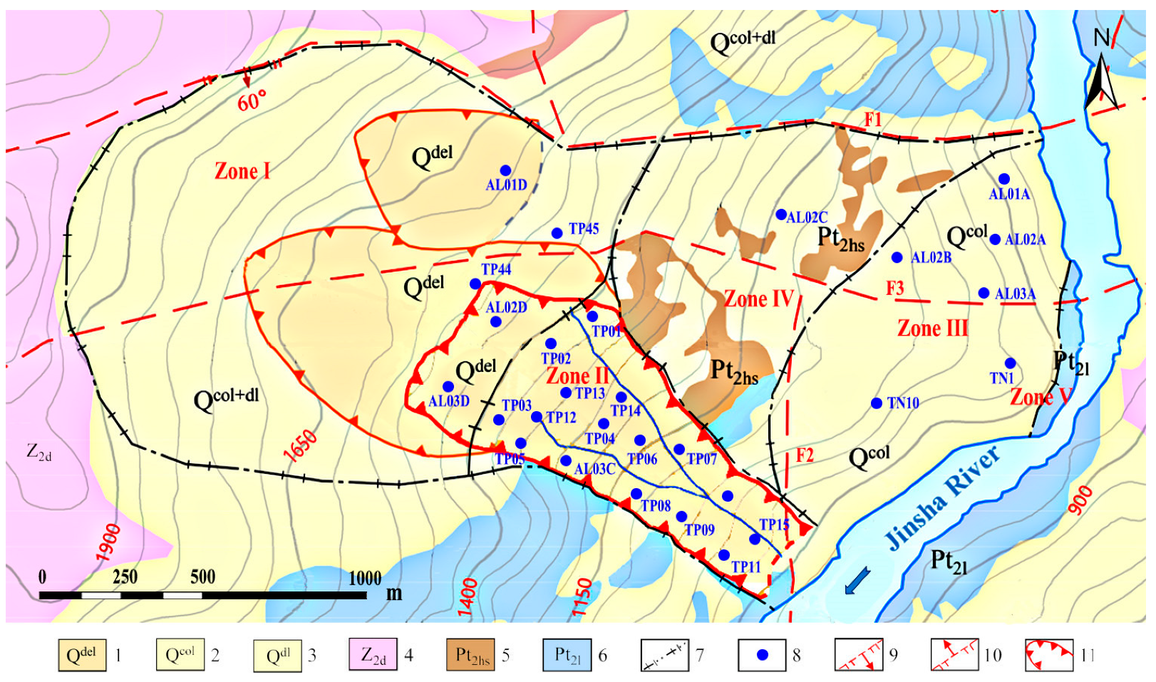
The landslide toe (leading edge) is curved and flows out of a 225 ° circular arc. The elevation of the toe ranges from 820 to 850 m, and the crown (uppermost edge) of the landslide ranges from 1900 to 2200 m. The landslide occurred on the left bank of Jinsha River, which drains the Wudongde area. The annual rainfall on the Jinpingzi landslide ranges from 452 to 665 mm, and the average slope is 26 ° . A topographic and lithological map is shown in Figure 2. There are three medium faults across the landslide site (F1, F2, and F3). Fortunately, there are all inactive. Middle Proterozoic phyllites constitute the bedrock. Quaternary landslide deposits are in the middle of the landslide, and the Quaternary colluvial deposits in the front change the path of Jinsha River. Middle Proterozoic dolomites are found on both sides of the riverbanks. According to the geological features of the Jinpingzi landslide, there are five districts in the landslide area: Zone I, Zone II, Zone III, Zone IV, and Zone V.
The strata of the Jinpingzi landslide are divided into double-layer structures. The hard, upper layer is composed of shale, marl, and dolomite, and the soft, lower layer is composed of limestone, marble, phyllite, and slate. Moreover, several geological fault structures cross the landslide area, which can easily lead to rock fragmentation and further aggravate sliding. The slide zone soil is purplish-red silty clay with a small amount of phyllite clastic rock. The soil is hard and plastic, and the thickness is 2 to 9 m.

2.2. Characteristics of the Jinpingzi Landslide

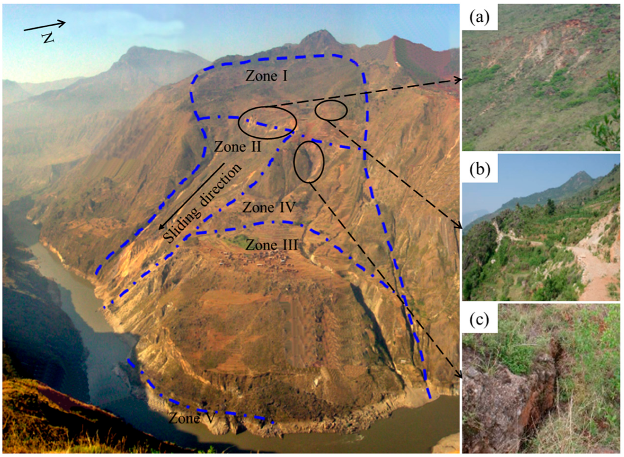
The volume of the Jinpingzi landslide is approximately 6.2 million m3, and the overburden thickness is 60 to 80 m. The noticeable features of the Jinpingzi landslide are depicted in Figure 3; the plane shape shows “a long neck and big belly” [35]. According to the geological conditions of the Jinpingzi landslide, it can be separated into five zones according to the bedrock beam in the sliding body, as shown by the blue line in Figure 3. Zone I is above the bedrock beam; Zone II is east of the bedrock beam; Zone III and Zone IV are in the middle; and Zone IV is in front of the bedrock beam, along the river. Zone II is the main sliding area according to the monitoring results.
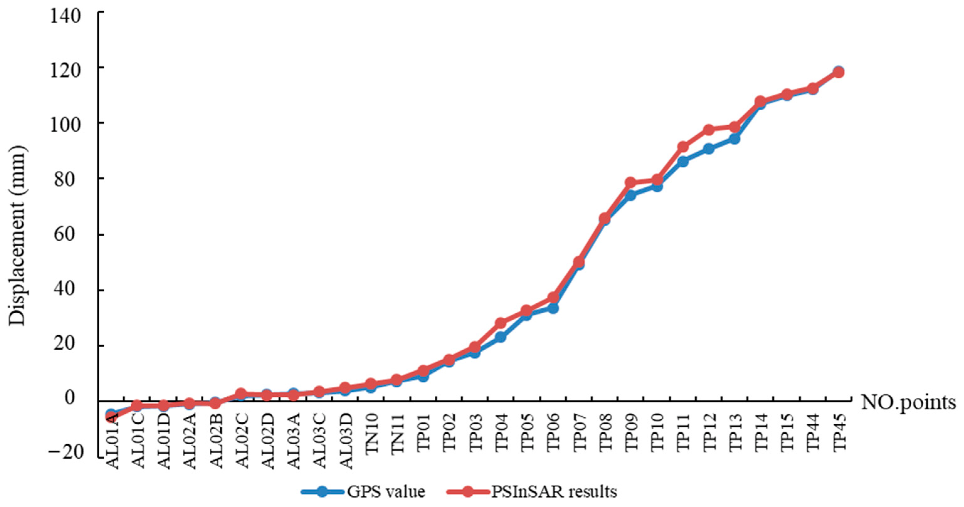
Radarsat-2 and global positioning system (GPS) data were used to obtain the displacement of the Jinpingzi landslide according to its position in July 2015 [36] The distribution map of the GPS points is shown in Figure 2. GPS points AL01D, AL02D, AL03D, TP44, and TP45 are in Zone I; TP01 to TP15 are in Zone II; AL01C is in Zone IV; and Zone III includes six GPS points (AL01A, AL02A, AL03A, AL02B, TN10, and TN11). The permanent scatterer interferometric synthetic aperture radar (PSInSAR) technique is an advanced InSAR technique based on permanent scatterer points to overcome time incoherence. Permanent scatterer points were used to extract the mean deformation value of the nearest 5 m to the GPS points. The monitoring results of GPS and the PSInSAR technique are shown in Figure 4. According to these results, the main deformation was caused by the traction creep of the overburden layer in Zone II (Figure 3a; GPS points from TP01 to TP15). The displacement ranges from 20 to 100 mm. GPS points TP44 and TP45 are located at the small-scale slump of the steep slope at the rear edge of the landslide (Figure 3b), and the movement starts in this area. Thus, the deformation is relatively large. Figure 3c shows a large crack forming with movement during the rainy season. Zone III is located at the foot of the slope, and the sliding soil banks up here. Thus, the monitoring results show negative values.

3. Numerical Model of Particle Flow Code 3D (PFC 3D)

The PFC 3D model is a discrete element method that uses the specific contact model of particles (i.e., 3D elements) to simulate the microscopic characteristics of rock–soil as an equivalent model [37,38]. The PFC 3D model consists of particles and walls. Walls are used to confine the boundary or the surface of landslides. Particles are used to simulate landslide soil by setting different micro-parameters. Particles are characterized by radius, density, coefficient of friction, and form of contact [39]. Moreover, particles are assigned gravity. Then, the landslide model can be modulated using the coefficient of friction and connection among particles under external forces. It is a dynamic process of the interactions among particles used in the PFC 3D model to achieve balance. Newton’s second law, F = ma, represents the relationship between force and displacement. Thus, Newton’s second law is used to calculate the motion and rotation of particles when the contact force of particles is unbalanced [40]. The gravity and force of adjacent particles change in the process of particle motion. Therefore, the contact force and torque of particles is calculated based on the relationship of force and displacement.

3.1. Micro-Parameters of PFC3D

In the PFC 3D model, the micro-strength parameters and the contact among particles are used to represent the characteristics of rock–soil mass. However, there is no direct calculation for transforming the macro-strength parameters of rock–soil mass into micro-strength parameters, and there is a nonlinear relationship between these two parameter types [31]. In the current study, to obtain the micro-strength parameters of the rock–soil mass of the Jinpingzi landslide, strength reduction theory (SRT) was used in uniaxial compression tests with 3259 particle units, as shown in Table 1. Further, a nonlinear relationship model was established between macro- and micro-parameters. The macro-parameters were the modulus of elasticity ( E = 38.5 M P a ) , Poisson’s ratio ( υ = 0.175 ), and normal stress ( σ = 82.6 M P a ). The obtained stress–strain curves are shown in Figure 5. Meanwhile, laboratory uniaxial compression tests were used to obtain the macro-strength parameters that carry soil materials along the landslide. The results of these parameters are as follows: E = 38.3 M P a ,   υ = 0.174 , and σ = 82.56   M P a . The macro-strength parameters obtained with two methods are very similar. The parallel contact-bond model was chosen to represent the acting force in the macro-strength test. Thus, the calculated micro-parameters in Table 1 could be used in the PFC 3D model based on SRT applied to the Jinpingzi landslide. The particle radii ranged from 3.75 to 6.25, and the particle and bond normal-to-shear stiffness ratios are represented by K = K = p b _ k n p b _ k s , respectively.

3.2. Strength Reduction Theory (SRT)

Owing to rainfall, earthquakes, and other external factors, the cohesion and internal friction angle of the slope soil constantly decrease due to the continuous action of rainfall infiltration or horizontal seismic force. Thus, the shear strength of soil and the sliding resistance of the slope body tend to decrease until failure. SRT is a simulation theory for slope stability analysis based on this principle and can be used to simulate the entire landslide process from the beginning to instability failure [37].
SRT reduces the shear strength of soil by reducing its material parameters (such as the angle of internal friction and cohesion) until the actual stress and slope reach the limit equilibrium state [41]. The reduction coefficient ( R ) is an important parameter for stability evaluation and can be expressed as
R = c c = tan φ t a n φ
where c is the initial cohesion, c′ is the reduced cohesion, φ is the internal friction angle, and φ is the reduced internal friction angle.
In the PFC 3D model, the internal failure mechanism of the soil was simulated using the bond mode among particles, including parallel and contact bonds. The parallel-bonded landslide can not only transfer force, but also transfer moment, which simulates the tension, shear, and bending moment among particles during landslide movement. Using SRT, the parallel-bond strength before the particle is reduced until the bond strength reaches a critical value to determine the stability state of the slope. The reduction coefficient ( R ) can be expressed as
R = p b _ k n p b _ k n = p b _ k s p b _ k s = f f
The parallel-bond strength among particles includes bond normal strength ( p b _ k n ), bond tangential strength ( p b _ k s ), and friction coefficient ( f ). When the slope body enters an unstable state, the bond strength determines critical bond normal strength ( p b _ k n ), critical bond tangential strength ( p b _ k s ), and friction coefficient ( f ).

3.3. Generation of the Jinpingzi Landslide Model

The discrete element method has advantages in simulating the discontinuous medium method and is suitable for simulating landslide kinetic features [42]. However, the scale of landslides is generally large, and the number of particles generated in the landslide area is very large, both of which seriously affect the calculation efficiency of the model. Of the entire slope, the region above the sliding surface is the sliding body area, and that below the sliding surface is considered non-sliding. Therefore, particles only need to be included above the sliding surface, which can significantly reduce the number of particles and improve the calculation efficiency.
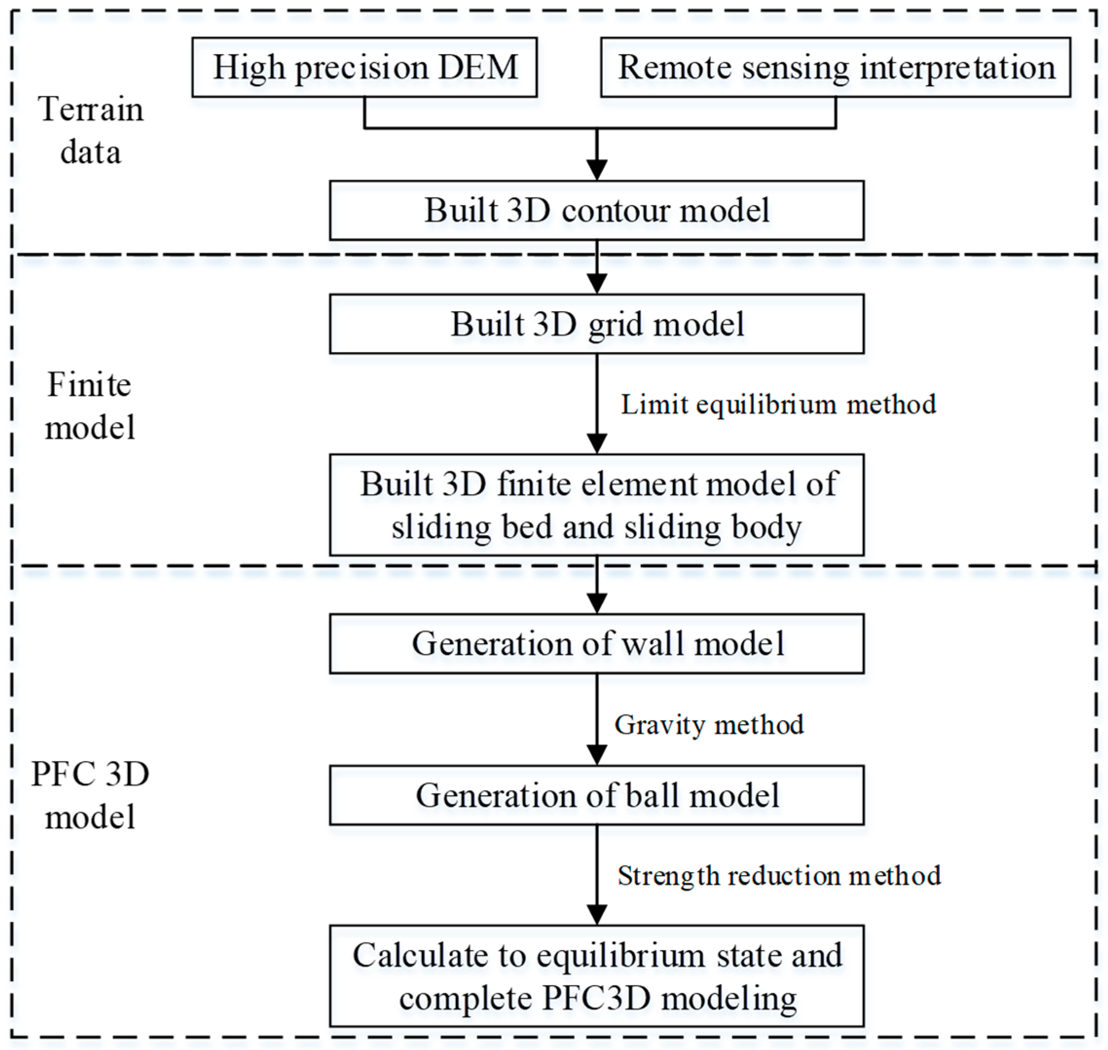
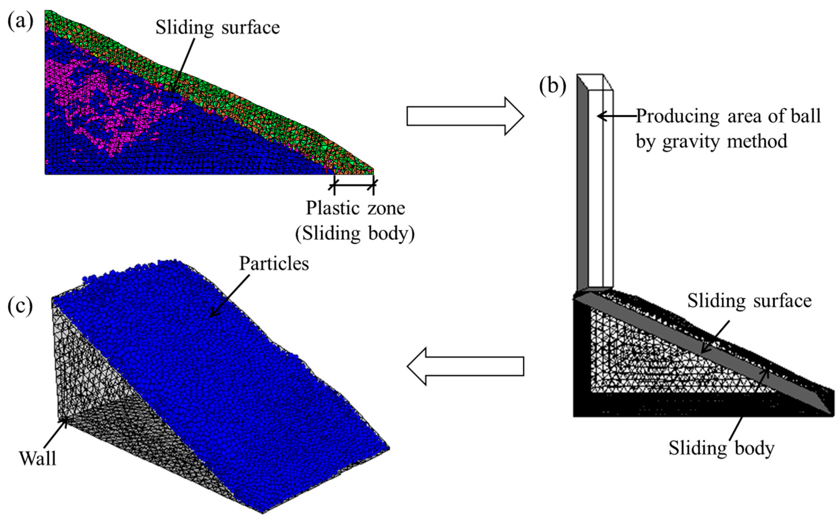
The sliding surface and bed were represented using the rigid wall model in the construction of the landslide model. As shown in Figure 6, the first step was to extract digital elevation model (DEM) data and conduct remote sensing interpretation to construct the finite element model (Figure 7a). Subsequently, SRT was adopted to obtain the sliding failure surface, which is the plastic zone of the Jinpingzi landslide, based on the finite element model using FLAC 3D (Fast Lagrangian Analysis of Continua in 3 Dimensions) software. As the reduction coefficient increased, the plastic zone expended until a through crack was formed on the slope, which was the sliding surface. The green area depicted in Figure 7a represents this sliding surface. In addition to the particle elements, the model also included wall elements as boundary conditions. The finite element model was transformed into the wall element structure of the PFC 3D model to impose boundary constraints around the slope, and the slip surface was separately established in the wall element structure. Finally, the sphere elements filled the gap between the slip surface and landslide surface.
In this model, the gravity method was used to generate ball particles, and a quadrilateral wall unit was built on top of the landslide to generate ball particles. By setting the gravity, the balls slid along the slope until the entire sliding zone was filled, as shown in Figure 7b. The bond among particles and the particle size was set according to the micro-parameters of the model. The particle size of the model ranged from 3.75 to 6.25 cm, with an average particle size of 5 cm. A total of 22,488 spherical elements were generated in the 3D sliding plane. The particle flow model of the Jinpingzi landslide is shown in Figure 7c, with the micro-parameters having only been applied to the particles above the sliding surface. Moreover, to simulate the sliding of soil on the surface of the landslide, the spheres on the surface of the landslide could freely slide along the slope without constraint. Therefore, it was necessary to delete the wall element on the landslide surface, allowing the spherical particles to slide freely along the slope under force without being constrained by the wall element.

3.4. Stability Analysis Based on Displacement Vector Angle (DVA)

Displacement is a vector value that includes magnitude and direction. The displacement value of the landslide can be directly monitored, but it is difficult to detect changes in the displacement direction. He et al. (2003) [43] proposed the concept of DVA. The DVA of landslide displacement refers to the inclination angle of the main sliding line, which indicates the vertical orientation of landslide body displacement. The DVA was introduced to study the change in landslide direction. As shown in Figure 8, in the 3D model, the DVA can be represented by the average displacement in the X- (D(x)), Y- (D(y)), and Z-directions (D(z)), as follows:
S m k x = D m k x 2 + D m k y 2
S m k z = D m k ( z )
α m k = a r c t a n S m k ( z ) S m k ( x ) ( m t , k n )
where S m k x is the horizontal displacement of point k at time m, representing the resultant displacement in the X- and Y-directions; and S m k z is the vertical displacement of point k in meters. Thus, the DVA can be represented by the horizontal and vertical displacements. N monitoring points can form the space–time matrix:
α m n = α 1 1 ( θ ) α m 1 ( θ ) α 1 n ( θ ) α m n ( θ )
In Newton’s second law, F = m a = m ( v / t ) , v represents the difference in the displacement rates between two adjacent time series. This implies that the directions of F and v are the same, which means that the change direction of F is followed by the change direction of v . Therefore, the stability state of the landslide can be predicted by analyzing the dynamic change direction of the displacement vector before and after the two periods. As shown in Figure 9, α 1 and α 2 represent the DVAs in the two consecutive periods. When the velocity gradually increases, as shown in Figure 9a, when α > 0 and v > 0 , the lower soil is compressed by the upper soil due to sliding force F , and the DVA changes from small to large. The slope is subjected to tensile stress. As shown in Figure 9b, when α = 0   a n d   v > 0 , the DVA is relatively stable; the slope slides overall; and the landslide is in the constant deformation stage. As shown in Figure 9c, when α < 0 and v > 0 , the DVA changes from large to small. The slope is subjected to squeezing and shearing in the stress state due to sliding force F . When the sliding surface is in a plastic state, the surface DVA of the slope is mutated. This mutation inevitably causes the DVA to increase or decrease. The DVA abruptly decreases in the extruded shear outlet region and abruptly increases in the tensioning and loosening zones. Thus, the changes in the DVA reflect the changes in the force direction and displacement of the slope body.

4. Simulation Results

The simulation results show that the bond strength among soil particles in the initial equilibrium state was gradually reduced by different reduction factors until the strength reduction stopped at 20,000 steps. After moving along the slope, these particles accumulated in the river channel at the toe of the slope. The river was incised by sliding particles, and barrier lakes were formed.

4.1. Kinetic Features of the Jinpingzi Landslide

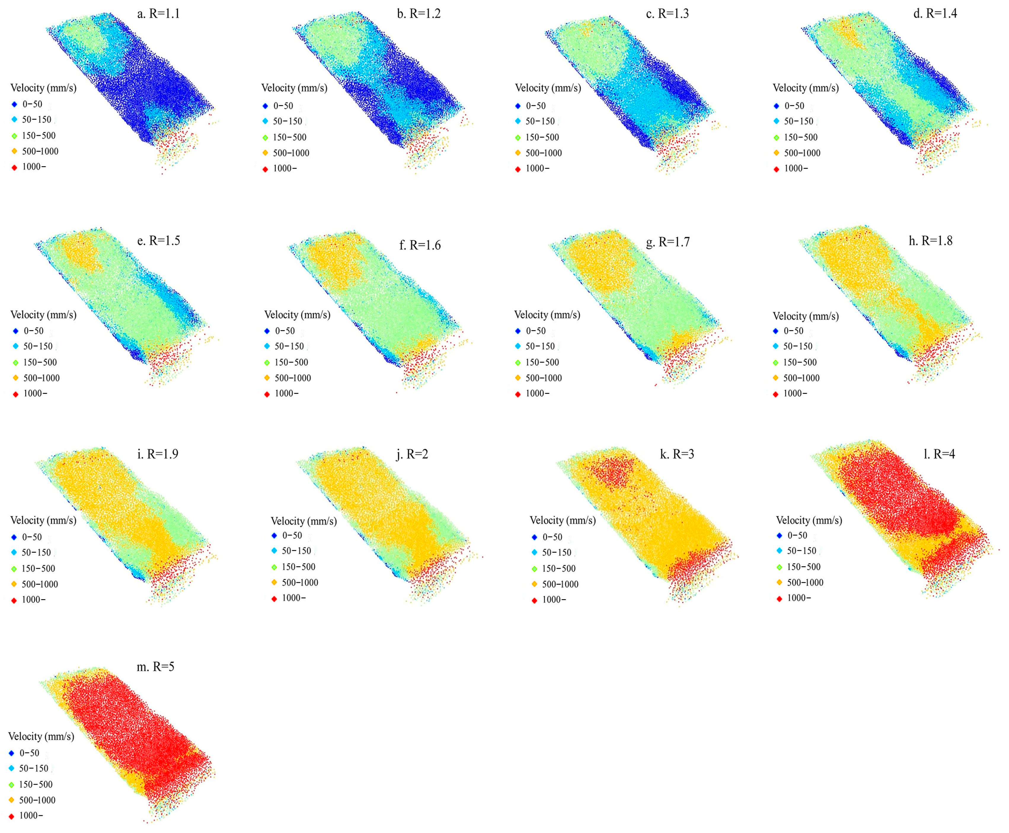
The simulation results with different reduction coefficients are shown in Figure 10. The reduction coefficients ranged from 1.1 to 5; when the reduction coefficient was small (1.1–1.4), the landslide began to deform under the influence of gravity due to the reduction in the bond strength among particles (Figure 10a–d). The particles were dark blue to light blue, which means that the displacement increased. The movement began at the front and rear edges of the slope, which is consistent with reality (Figure 10e–h). With an increase in R, the displacement continued to increase until it ran through the entire sliding surface. Meanwhile, more and more particles turned to yellow. The sliding surface gradually moves to the deeper area. As shown in Figure 10i–m, the sliding region continued to expand downward along the landslide. Most particles slid along the slope with very fast velocity (red balls) and then fell into Jinsha River.
The sliding surface gradually coalesced after the initial deformation stage, and the landslide was in the constant deformation stage with a low velocity and did not enter the accelerated deformation stage. This phenomenon occurred because the reduction coefficient was small; thus, the simulation required a longer time for the landslide to enter the stage of accelerated deformation. As the reduction coefficient increased, the bond strength decreased, and the time from the initial deformation stage to the constant deformation stage of the landslide decreased. Meanwhile, the sliding surface extended in depth (Figure 10a–m). The sliding surface was formed as shown in Figure 10c; as shown in the figure, the light-blue particles connected the leading and rear edges. With the increase in R, the velocity of the first sliding surface was large and the sliding surface with light blue particles was extended in depth. After the constant deformation stage, the landslide entered the final accelerated deformation stage. Finally, Jinsha River was blocked by particles, and a barrier lake was formed. The different reduction coefficients simulated different time periods of the processing of the landslide. The simulation results are consistent with GPS and InSAR monitoring.
The cumulative displacement and velocity curves are shown in Figure 11. In Figure 11a, it can be observed that the cumulative displacement of all particles on the slope surface increased over time. The rate of displacement increased as the reduction coefficient increased. According to the growth trend, when R = 5, the maximum of cumulative displacement was approximately 10 m. When R = 1.1–1.3, the velocity of all particles rapidly increased at first and then slowly decreased with time. The velocity peaked at 0.3 × 10⁴ steps, approximately 120 mm/s. After that, the velocity decreased to 20, 42, and 86 mm/s and then stabilized at 1.6 × 10⁴ steps (Figure 11b). The landslide then entered a constant deformation stage, and the sliding velocity was stable. With the increase in the reduction coefficient, the duration of the constant deformation stage decreased. At R = 1.4, the first peak velocity was still approximately 120 mm/s, but the final accelerated deformation stage started at 0.6 × 10⁴ steps.
The critical velocity represents the velocity of the boundaries from the constant deformation stage to the final accelerated deformation stage, meaning that the landslide enters the final accelerated deformation stage after reaching its critical velocity. From Figure 11b, the critical velocity increased with the increase in R. Further, the first turning point of critical velocity occurred at R = 1.4, which is the indication of the change from the initial deformation stage to the constant deformation stage. The second turning point of critical velocity occurred at R = 3, with the final accelerated deformation stage starting at 0.45 × 10⁴ steps, and the critical velocity rapidly increased.

4.2. Stability Analysis of Jinpingzi Landslide

In Figure 9, it can be seen that the changes in the DVA and velocity reflect the different stability states of slow-moving landslides. According to mutation theory, the instantaneous abnormal change in parameters can be used as the basis for the change in the motion state. Thus, the critical velocity of the slow-moving landslide can be said to represent the abrupt velocity from the constant deformation stage to the final accelerated deformation stage. In this study, the 3D simulation displacement results were converted to DVA values using Equations (3)–(6). Thus, the two-parameter instability criterion was established according to the relationship among DVA, critical velocity, and reduction coefficient.
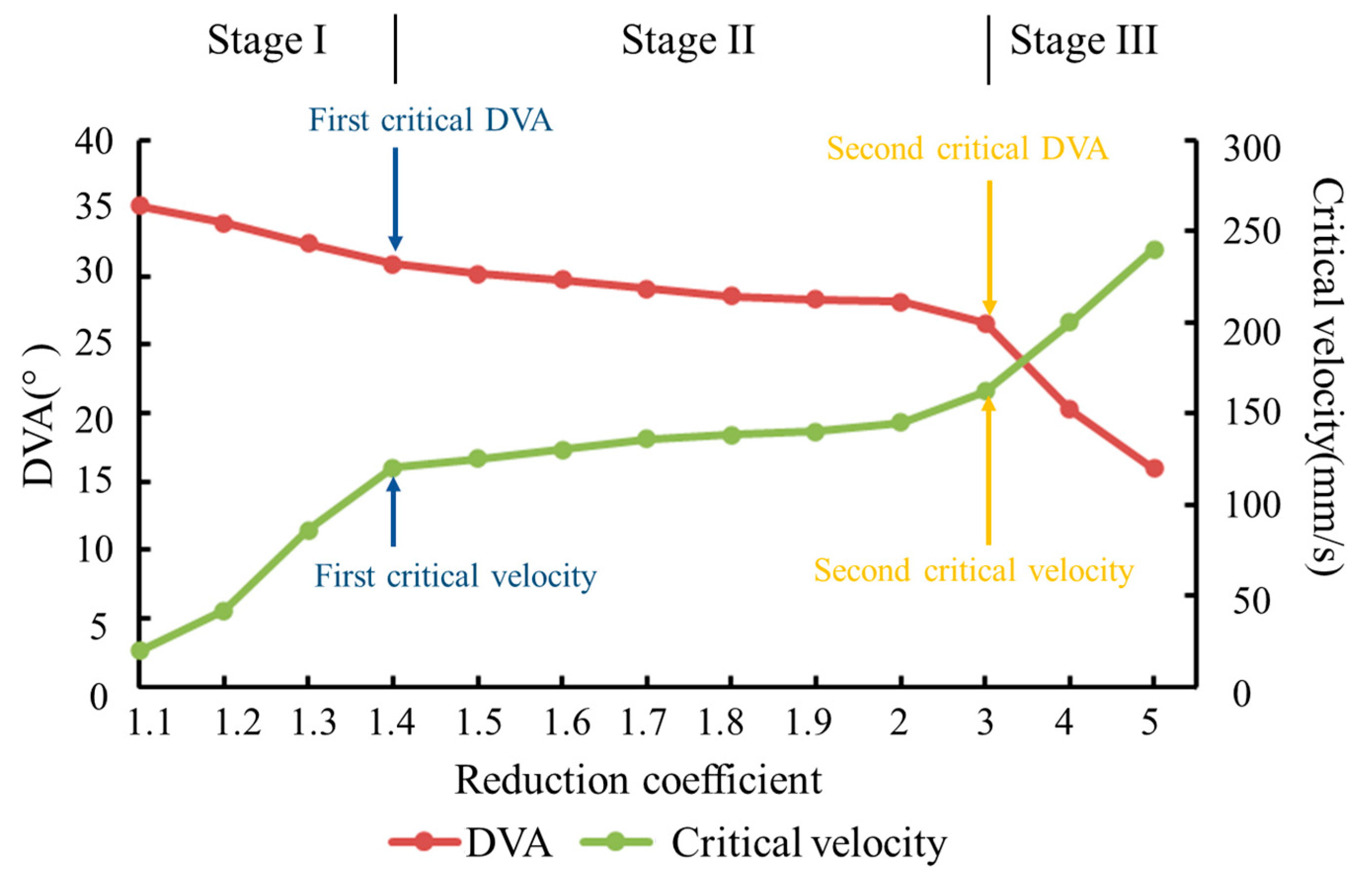
The average DVA and critical velocity curves of the Jinpingzi landslide with different reduction coefficients were calculated. Figure 12 shows the relationship between the average DVA and the reduction coefficient. The DVA decreased as the reduction factor gradually increased. This means that the angle between the inclination angle and the vertical direction became increasingly small, indicating that the landslide was slowing down. The first and second curve mutations occurred when the reduction coefficients was 1.4 (blue arrows in Figure 12) and 3 (orange arrows in Figure 12), respectively. At the first mutation point, the landslide moved from the initial accelerated deformation stage to the constant deformation stage. The inflection point of the DVA was 30.89°. At the second mutation point, the landslide entered the final accelerated deformation stage, and instability could occur at any time. The DVA of the second mutation point was 26.59°, which can be considered the critical DVA of the landslide.
Figure 12 shows the relationship between the average velocity and the reduction coefficient. The velocity increased as the reduction factor gradually increased. The occurrence time of the curve mutation was consistent with that of the DVA. Therefore, the critical velocity thresholds of the Jinpingzi landslide were 120 mm/s, from Stage I to Stage II, and 162 mm/s, from Stage II to Stage III. In Figure 12, the displacement features of Jinpingzi landslide are in accordance with those of a slow-moving landslide. Thus, it can be confirmed that the Jinpingzi landslide is a typical slow-moving landslide. Further, the numerical simulation results of the PFC3D model are consistent with the movement characteristics of slow-moving landslides. According to the above theory, the stability state of the Jinpingzi landslide can be determined with the continuous monitoring of displacement and velocity.

5. Discussion

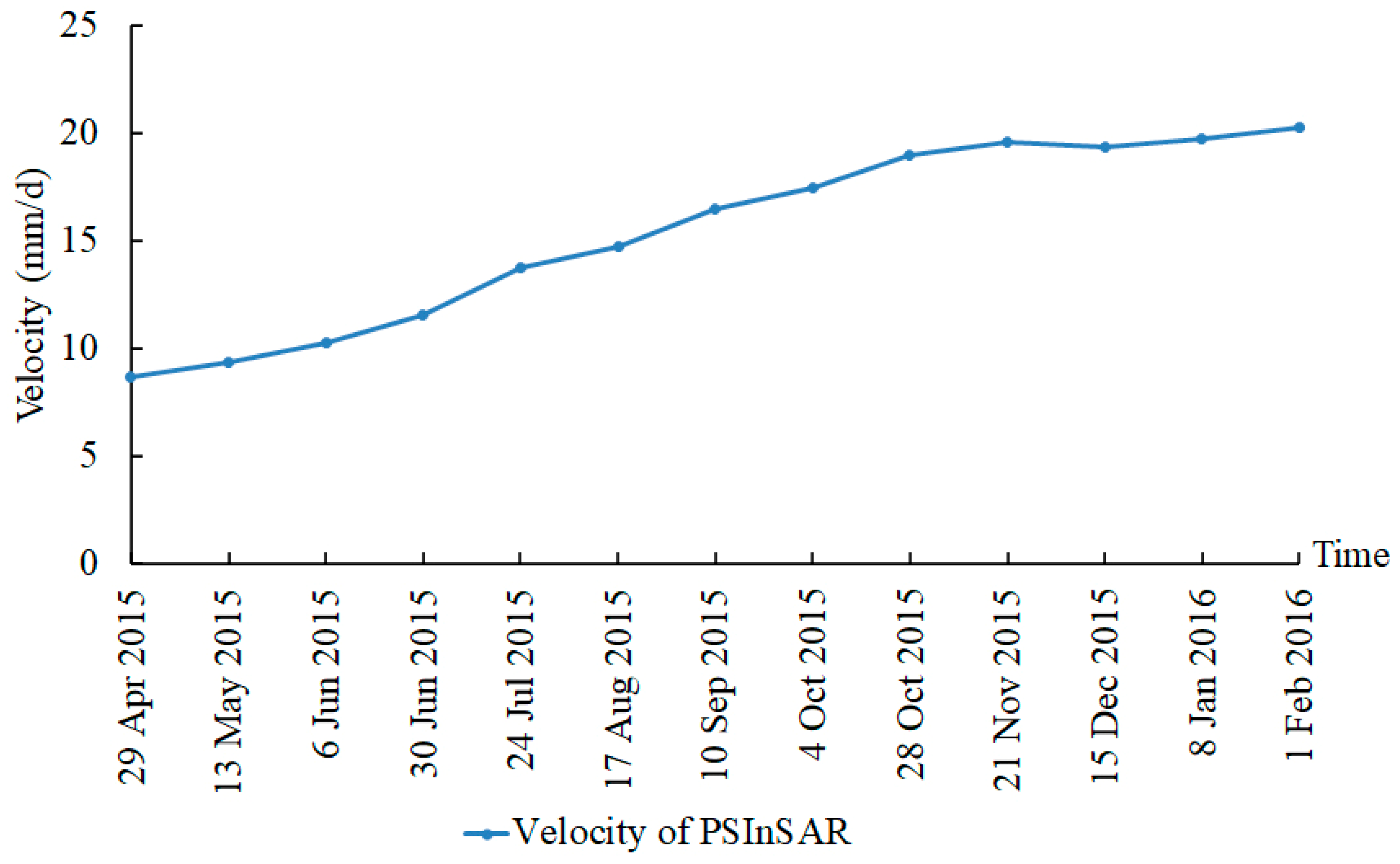
This research is based on the PFC method to simulate the kinetic features of a slow-moving landslide. The gravity method was used to generate particles to construct the landslide body, and SRT was used to simulate the movement mechanism of the entire process using different reduction coefficients. Figure 13 shows the average velocity monitoring results from 2015 to 2016 using the PSInSAR technique. It can be seen that the velocity gradually increased in the rainy season (from June to October), and the velocity was approximately 20 mm/d. In contrast, according to the simulation results of the PFC3D model, the kinetic features of the landslides were consistent with Stage I of slow-moving landslides, which proves the correctness of the model. Due to only one parameter having been considered in the numerical simulation, external factors such as rainfall were not taken into account. Nevertheless, although the velocity value obtained using PSInSAR was different from the simulation result, the movement trend of the landslide was consistent. Therefore, the critical displacement can be identified with continuous monitoring.
This research was based on SRT and the coupled two-parameter instability criterion to analyze the kinetic features and stability of the Jinpingzi landslide. Typically, the single-parameter approach is used, such as displacement value [44], velocity [45], vertical displacement direction rate [46], or precipitation [47], which is applied to one landslide or one kind of landslide. When using the single-parameter instability criterion, it can only be used for the originally studied landslide. Most scholars choose displacement as the instability criterion. However, displacement is a vector physical quantity that can be expressed using DVA and velocity. Velocity represents the change in value, and DVA represents the change in direction. Moreover, for regional landslides, the single-parameter approach could potentially misrepresent the situation under different geological conditions and climate factors. In contrast, the two-parameter instability criterion is suitable for all landslide types.
In this paper, the contour model was extracted using remote sensing interpretation and DEM, and the ball model was used to construct the landslide body. However, the finite element method for determining the sliding surface could reduce the number of balls and improve the computation speed. In this method, the position of the sliding surface could change owing to the influence of external conditions; thus, the second sliding surface could not be obtained, and the multistage sliding surface could not be considered. Moreover, the parallel-bond strength coefficients were reduced with the same reduction coefficient, which is inconsistent with the actual situation. In the future, multistage landslide sliding surfaces and different reduction coefficients for different parameters will be studied based on compression tests and field experiments.

6. Conclusions

Taking the Jinpingzi landslide in the Wudongde area as the study target, this research investigated the kinetic features and stability analysis of a slow-moving landslide, including displacement, velocity, and DVA. Based on remote sensing interpretation, the DEM was used to generate a contour model of the landslide, and the micro-parameters of the landslide model were obtained using uniaxial compression. The finite element model was used to extract the sliding body of the landslide. Then, the PFC3D model of the Jinpingzi landslide was established, and the motion process of the DVA and critical velocity were simulated from the beginning to the instability stage based on SRT. The simulation results are as follows.
(1) Sliding started at the front and rear edges of the Jinpingzi landslide under reduced parallel-bond strength; the displacement of the rear edge was the largest, which is in agreement with the actual monitoring results of the landslide. With the transfixion of the sliding surface, the velocity of the landslide gradually increased until it became unstable. The kinetic features of the Jinpingzi landslide conformed to the slow-moving landslide, which blocked the Jinsha River basin, formed a barrier lake, and affected the safety of the Wudongde hydropower dam.
(2) According to the DVA curves, the critical velocity and reduction coefficient showed that the DVA of the landslide decreased as the reduction coefficient increased, and the critical velocity increased as the reduction coefficient increased. The mutation points of the two curves occurred when the reduction coefficients were 1.4 and 3, respectively. When the reduction coefficient was 1.4, the DVA was 30.8°, and the critical velocity was 152 mm/s. When the reduction coefficient was 3, the DVA was 28.15°, and the critical velocity was 200 mm/s.
(3) According to Newton’s second law and catastrophe theory, changes in DVA and velocity can reflect the stability state of a landslide. In this study, a two-parameter instability criterion is proposed, and the stability state can be determined with the continuous monitoring of displacement and velocity. This method provides a theoretical basis for stability analysis and disaster prevention.

Author Contributions

Conceptualization, J.H. and M.X.; methodology, J.H.; software, J.H.; validation, J.H., W.D. and M.X.; formal analysis, J.H.; investigation, J.H.; resources, J.H. and M.X.; data curation, J.H.; writing—original draft preparation, J.H.; writing—review and editing, J.H. and W.D.; visualization, W.D.; supervision, M.X.; project administration, J.H.; funding acquisition, J.H. All authors have read and agreed to the published version of the manuscript.

Funding

This work was supported by Zhejiang Provincial Natural Science Foundation of China under grant No. LQ02D020001, Scientific research project of Zhejiang Provincial Department of Education (No. Y202146383), and Youth foundation of Zhejiang University of Science and Technology (No. 2021QN059).

Data Availability Statement

There are no new data were created.

Conflicts of Interest

The authors declare that there are non-financial interest or personal relationships that are directly or indirectly related to the work submitted for publication.

References

  1. Wan, S.; Lei, T.C.; Chou, T.Y. A novel data mining technique of analysis and classification for landslide problems. Nat. Hazards 2010, 52, 211–230. [Google Scholar] [CrossRef]
  2. Vinueza, A.U.; Handwerger, A.L.; Bakker, M.; Bogaard, T. A new method to detect changes in displacement rates of slow-moving landslides using InSAR time series. Landslides 2022, 19, 2233–2247. [Google Scholar] [CrossRef]
  3. Nefeslioglu, H.A.; Gokceoglu, C.; Sonmez, H.; Gorum, T. Medium-scale hazard mapping for shallow landslide initiation: The Buyukkoy catchment area (Cayeli, Rize, Turkey). Landslides 2011, 8, 459–483. [Google Scholar] [CrossRef]
  4. Luo, G.; Hu, X.; Gu, C.; Wang, Y. Numerical simulations of kinetic formation mechanism of Tangjiashan landslide. J. Rock Mech. Geotech. Eng. 2012, 4, 149–159. [Google Scholar] [CrossRef] [Green Version]
  5. Jeong, S.W. The viscosity of fine-grained sediments: A comparison of low- to medium-activity and high-activity clays. Eng. Geol. 2013, 154, 1–5. [Google Scholar] [CrossRef]
  6. Fan, X.; Qiang, X.; Scaringi, G.; Dai, L.; Havenith, H.B. Failure mechanism and kinematics of the deadly June 24th 2017 Xinmo landslide, Maoxian, Sichuan, China. Landslides 2017, 14, 2129–2146. [Google Scholar] [CrossRef]
  7. Intrieri, E.; Raspini, F.; Fumagalli, A.; Lu, P.; Conte, S.D.; Farina, P.; Allievi, J.; Ferretti, A.; Casagli, N. The Maoxian landslide as seen from space: Detecting precursors of failure with sentinel-1 data. Landslides 2018, 15, 123–133. [Google Scholar] [CrossRef] [Green Version]
  8. Kundu, J.; Sarkar, K.; Ghaderpour, E.; Scarascia Mugnozza, G.; Mazzanti, P. A GIS-Based Kinematic Analysis for Jointed Rock Slope Stability: An Application to Himalayan Slopes. Land 2023, 12, 402. [Google Scholar] [CrossRef]
  9. Huang, B.; Yin, Y.; Wang, S.; Chen, X.; Liu, G.; Jiang, Z.; Liu, J. A physical similarity model of an impulsive wave generated by gongjiafang landslide in Three Gorges Reservoir, China. Landslides 2014, 11, 513–525. [Google Scholar] [CrossRef]
  10. He, C.; Hu, X.; Tannant, D.D.; Tan, F.L.; Zhang, Y.M.; Zhang, H. Response of a landslide to reservoir impoundment in model tests. Eng. Geol. 2018, 247, 84–93. [Google Scholar] [CrossRef]
  11. Du, W.Q. Effects of directionality and vertical component of ground motions on seismic slope displacements in newmark sliding-block analysis. Eng. Geol. 2018, 239, 13–21. [Google Scholar] [CrossRef]
  12. Michele, F.D.; Cantagallo, C.; Spacone, E. Effects of the vertical seismic component on seismic performance of an unreinforced masonry structures. Bull. Earthq. Eng. 2020, 18, 1635–1656. [Google Scholar] [CrossRef]
  13. Jiang, J.W.; Ehret, D.; Xiang, W.; Rohn, J.; Huang, L.; Yan, S.J.; Bi, R.W. Numerical simulation of Qiaotou Landslide deformation caused by drawdown of the Three Gorges Reservoir, China. Environ. Earth Sci. 2011, 62, 411–419. [Google Scholar] [CrossRef]
  14. Huang, T.; Ding, M.T.; She, T.; Tian, S.T.; Yang, J.T. Numerical simulation of a high-speed landslide in Chenjiaba Beichuan, China. J. Mt. Sci. 2017, 14, 2137–2147. [Google Scholar] [CrossRef]
  15. Hu, Y.X.; Yu, Z.Y.; Zhou, J.W. Numerical simulation of landslide generated waves during the 11 October 2018 Baige landslide at the Jinsha River. Landslide 2020, 17, 2317–2328. [Google Scholar] [CrossRef]
  16. Cheng, Q.; Yang, Y.H.; Du, Y. Failure mechanism and kinematics of the Tonghua landslide based on multidisciplinary pre- and post- failure data. Landslides 2021, 18, 3857–3874. [Google Scholar] [CrossRef]
  17. Niu, Q. Secondary Development of Loess Creep Model Based on FLAC3D and Application on Time Prediction of Landslide Sliding; Lanzhou University of Technology: Lanzhou, China, 2014. (In Chinese) [Google Scholar]
  18. Bru, G.; Fernández-Merodo, J.A.; García-Davalillo, J.C.; Herrera, G.; Fernández, J. Site scale modeling of slow-moving landslides, a 3D viscoplastic finite element modeling approach. Landslides 2018, 15, 257–272. [Google Scholar] [CrossRef]
  19. Kafle, L.; Xu, W.J.; Zeng, S.Y.; Nagel, T. A numerical investigation of slope stability influenced by the combined effects of reservoir water level fluctuations and precipitation: A case study of the bianjiazhai landslide in China. Eng. Geol. 2022, 297, 106508. [Google Scholar] [CrossRef]
  20. Lei, Y.; Wang, S. Stability analysis of jointed rock slope by strength reduction based on UDEC. Rock Soil Mech. 2006, 10, 1693–1697. (In Chinese) [Google Scholar]
  21. Zhang, L.; Tang, H.; Xiong, C.; Huang, L.; Zou, Z. Movement process simulation of high-speed long-distance Jiweishan landslide with PFC 3D. Chin. J. Rock Mech. Eng. 2012, 31, 2601–2611. (In Chinese) [Google Scholar]
  22. Hu, X.; Fan, X.; Tang, J. Accumulation characteristics and energy conversion of high-speed and long-distance landslide on the basis of DEM: A case study of Sansicun Landslide. J. Geomech. 2019, 4, 527–535. (In Chinese) [Google Scholar]
  23. Li, Z.; Zhou, F.; Han, X.; Chen, J.; Bao, Y. Numerical simulation and analysis of a geological disaster chain in the Peilong valley, se Tibetan Plateau. Bull. Eng. Geol. Environ. 2021, 80, 3405–3422. [Google Scholar] [CrossRef]
  24. Shiu, W.J.; Lee, C.F.; Chiu, C.C.; Weng, M.C.; Yang, C.M.; Chao, W.A.; Liu, Y.L.; Lin, C.H.; Huang, W.K. Analyzing landslide-induced debris flow and flow-bridge interaction by using a hybrid model of depth-averaged model and discrete element method. Landslide 2023, 20, 331–349. [Google Scholar] [CrossRef]
  25. Zhang, J.M.; Zhou, Z.; Lin, F.; Yang, Q.G.; Luo, Y. Failure mechanism of a slow-moving landslide on September 27, 2020, in Chang Nong Village, Guangxi, China. Landslides 2021, 18, 2575–2592. [Google Scholar] [CrossRef]
  26. Zhang, N.; Zhang, J.W.; Mu, Q.Y.; Yang, Z.J. Numerical modeling of the Xinmo landslide from progressive movement to sudden failure. Environ. Earth Sci. 2021, 80, 355. [Google Scholar] [CrossRef]
  27. Jiang, S.; Wang, Y.F.; Tang, C.; Liu, K. Long-term kinematics and mechanism of a deep-seated slow-moving debris slide near Wudongde hydropower station in Southwest China. J. Mt. Sci. 2018, 15, 364–379. [Google Scholar] [CrossRef]
  28. Shah, S.S.; Mathur, S.; Chakma, S. Numerical modeling of one-dimensional variably saturated flow in a homogeneous and layered soil–water system via mixed form Richards equation with Picard iterative scheme. Model. Earth Syst. Environ. 2022. peer-reviewed. [Google Scholar] [CrossRef]
  29. Sutaih, G.H.; Aggour, M.S. A numerical model for analysis of a pile subjected to horizontal dynamic loading in elastic homogeneous and nonhomogeneous soils. Arab. J. Geosci. 2022, 15, 1085. [Google Scholar] [CrossRef]
  30. Chen, Z.; Song, D. Numerical investigation of the recent Chenhecun landslide (Gansu, China) using the discrete element method. Nat. Hazards 2021, 105, 717–733. [Google Scholar] [CrossRef]
  31. Li, Z.; Rao, Q.H. Quantitative determination of PFC3D microscopic parameters. J. Cent. South Univ. 2021, 28, 911–925. (In Chinese) [Google Scholar] [CrossRef]
  32. Yan, J.H.; Chen, J.P.; Zhou, F.J.; Li, Y.C.; Zhang, Y.W.; Gu, F.F.; Zhang, Y.S.; Li, Y.C.; Li, Z.H.; Bao, Y.D.; et al. Numerical simulation of the Rongcharong paleolandslide river-blocking event: Implication for the longevity of the landslide dam. Landslides 2022, 19, 1339–1356. [Google Scholar] [CrossRef]
  33. Hu, X.; Mei, H.; Zhang, H.; Li, Y.; Li, M. Performance evaluation of ensemble learning techniques for landslide susceptibility mapping at the Jinping county, southwest China. Nat. Hazards 2021, 105, 1663–1689. [Google Scholar] [CrossRef]
  34. Lu, W.Y.; He, C.C. Deformation Characteristics and Mechanism of Side Walls of Wudongde Hydropower Station. Geotech. Geol. Eng. 2022, 40, 4657–4671. [Google Scholar] [CrossRef]
  35. Mao, W.; Hei-Yan, R.U. Hazard evaluation for Jinpingzi landslide based on GIS and AHP method. Earth Environ. 2011, 39, 399–404. (In Chinese) [Google Scholar]
  36. Huang, J.X.; Xie, M.W.; Atkinson, P.M. Dynamic susceptibility mapping of slow-moving landslides using PSInSAR. Int. J. Remote Sens. 2020, 41, 7509–7529. [Google Scholar] [CrossRef]
  37. Chen, G.Q.; Li, H.; Wei, T.; Zhu, J. Searching for multistage sliding surfaces based on the discontinuous dynamic strength reduction method. Eng. Geol. 2021, 286, 10686. [Google Scholar] [CrossRef]
  38. Li, B.; Tang, H.; Gong, W.P.; Cheng, Z.; Li, T.Z.; Wang, L. Numerical study of the runout behavior of the Kamenziwan landslide in the Three Gorges Reservoir region, China. Landslides 2022, 19, 963–976. [Google Scholar] [CrossRef]
  39. Shi, C.; Li, D.J.; Chen, K.H.; Zhou, J.W. Failure mechanism and stability analysis of the Zhenggang landslide in Yunnan Province of China using 3D particle flow code simulation. J. Mt. Sci. 2016, 13, 891–905. [Google Scholar] [CrossRef]
  40. Potyondy, D.O. Simulating stress corrosion with a bonded-particle model for rock. Int. J. Rock Mech. Min. Sci. 2007, 44, 677–691. [Google Scholar] [CrossRef]
  41. Sun, W.; Wang, G.; Zhang, L. Slope stability analysis by strength reduction method based on average residual displacement increment criterion. Bull. Eng. Geol. Environ. 2021, 80, 4367–4378. [Google Scholar] [CrossRef]
  42. Wang, X.Q.; Xiao, L.; Zhao, J.K.; Ye, S.Q.; Wei, J.; Huang, X. Analysis of the formation mechanism of a landslide in the lacustrine sediment of the Diexi ancient dammed lake in the upper reaches of the Minjiang River. Bull. Eng. Geol. Environ. 2022, 81, 328. [Google Scholar] [CrossRef]
  43. He, K.Q.; Yang, J.B.; Wang, S.J. Displacement vector angle of colluvial slope and its significance. Chin. J. Rock Mech. Eng. 2003, 22, 1976–1983. (In Chinese) [Google Scholar]
  44. Qian, H.; Zhang, L.; Lan, J.; Wang, S. Analyses of critical sliding displacement of landslide induced by strong earthquake in mountainous area. Chin. J. Rock Mech. Eng. 2012, 31, 2619–2628. (In Chinese) [Google Scholar]
  45. Yang, Q.; Guan, M.; Peng, Y.; Chen, H. Numerical investigation of flash flood dynamics due to cascading failures of natural landslide dams. Eng. Geol. 2020, 276, 105765. [Google Scholar] [CrossRef]
  46. He, K.; Liu, H.; Guo, L.; Yuan, X.; Zhang, P. Innovative consideration of a directional appraisal parameter as destabilized criterion of the colluvial landslide. Environ. Earth Sci. 2019, 78, 685. [Google Scholar] [CrossRef]
  47. Hou, J.; Dou, M.; Zhang, Y.; Wang, J.; Li, G. An evaluation model for landslide and debris flow prediction using multiple hydrometeorological variables. Environ. Earth Sci. 2021, 80, 515. [Google Scholar] [CrossRef]
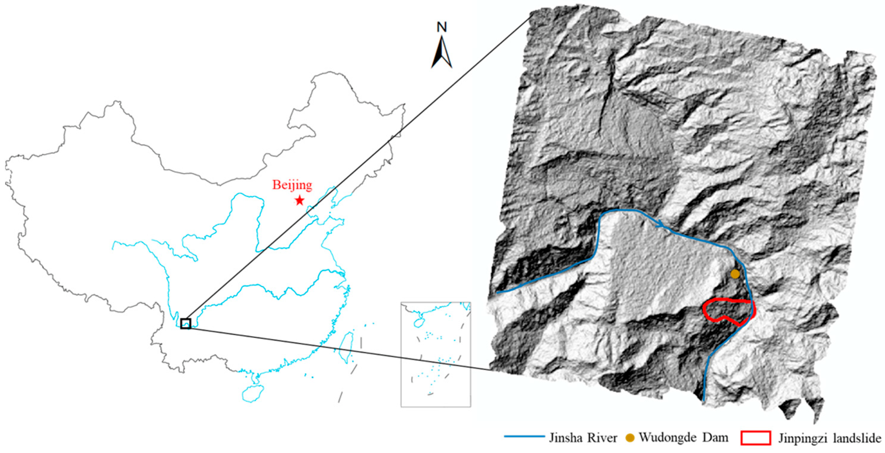
Figure 1. Location of the Jinpingzi landslide.
Land 12 00679 g001
Figure 2. Topographic and lithological map of the Jinpingzi landslide. (1. Quaternary landslide deposit; 2. Quaternary colluvial deposit; 3. Quaternary slope deposit; 4. Upper Sinian dolomite; 5. Middle Proterozoic phyllite; 6. Middle Proterozoic dolomite; 7. Boundaries of landslide and zone areas; 8. GPS point; 9. Normal fault; 10. Reversed fault; 11. Active Zone II area).
Land 12 00679 g002
Figure 3. Local features of the Jinpingzi landslide. (a) The main deformation of Zone II; (b) The small-scale slump of the steep slope at the rear edge of the landslide; (c) A large crack forming with movement.
Land 12 00679 g003
Figure 4. Monitoring results of GPS and permanent scatterer interferometric synthetic aperture radar (PSInSAR) data.
Land 12 00679 g004
Figure 5. Results of uniaxial compression test.
Land 12 00679 g005
Figure 6. Flowchart of particle flow code 3D (PFC3D) modeling.
Land 12 00679 g006
Figure 7. PFC 3D modeling for the Jinpingzi landslide: (a) FEM of the landslide; (b) The generation of wall model based on finite element model of the sliding bed; and (c) The generation of ball model in the sliding body.
Land 12 00679 g007
Figure 8. Schematic map illustrating the displacement vector angle (DVA).
Land 12 00679 g008
Figure 9. The relationship between DVA and sliding force F . (a) α > 0 and v > 0 ; (b) α = 0 a n d v > 0 ; (c) α < 0 and v > 0 .
Land 12 00679 g009
Figure 10. Kinetic features map of the Jinpingzi landslide with different reduction coefficients (R). (a) R = 1.1; (b) R = 1.2; (c) R = 1.3; (d) R = 1.4; (e) R = 1.5; (f) R = 1.6; (g) R = 1.7; (h) R = 1.8; (i) R = 1.9; (j) R = 2; (k) R = 3; (l) R = 4; (m) R = 5.
Land 12 00679 g010
Figure 11. (a) Displacement curves with different reduction coefficients. (b) Velocity curves with different reduction coefficients.
Land 12 00679 g011
Figure 12. Comparison of DVA, critical velocity, and reduction coefficient of the landslide.
Land 12 00679 g012
Figure 13. Velocity of the Jinpingzi landslide based on the PSInSAR technique.
Land 12 00679 g013
Table 1. Micro-strength parameters of the PFC 3D model.
ParameterDefinitionValue
RminMinimum particle radius (cm)3.75
RmaxMaximum particle radius (cm)6.25
Rmax/RminParticle radius ratio1.67
ρ Particle density (kg/m3)2150
K Particle normal-to-shear stiffness ratio0.33
K Parallel-bond normal-to-shear stiffness ratio0.33
E c Particle contact modulus (GPa)27.5
E c Bond effective modulus (GPa)27.5
f Micro-friction coefficient0.75
p b _ k n Bond normal strength (MPa)9.8
p b _ k s Bond tangential strength (MPa)29.7
Disclaimer/Publisher’s Note: The statements, opinions and data contained in all publications are solely those of the individual author(s) and contributor(s) and not of MDPI and/or the editor(s). MDPI and/or the editor(s) disclaim responsibility for any injury to people or property resulting from any ideas, methods, instructions or products referred to in the content.