Article

Monitoring the Rice Panicle Blast Control Period Based on UAV Multispectral Remote Sensing and Machine Learning

1
Nanjing Institute of Agricultural Mechanization, Ministry of Agriculture and Rural Affairs, Nanjing 210014, China
2
Graduate School of Chinese Academy of Agricultural Sciences, Beijing 100081, China
*
Authors to whom correspondence should be addressed.
Land 2023, 12(2), 469; https://doi.org/10.3390/land12020469
Submission received: 10 January 2023 / Revised: 7 February 2023 / Accepted: 10 February 2023 / Published: 14 February 2023
(This article belongs to the Section Land – Observation and Monitoring)

Abstract

:
The heading stage of rice is a critical period for disease control, such as for panicle blast. The rapid and accurate monitoring of rice growth is of great significance for plant protection operations in large areas for mobilizing resources. For this paper, the canopy multispectral information acquired continuously by an unmanned aerial vehicle (UAV) was used to obtain the heading rate by inversion. The results indicated that the multi-vegetation index inversion model is more accurate than the single-band and single-vegetation index inversion models. Compared with traditional inversion algorithms such as neural network (NN) and support vector regression (SVR), the adaptive boosting algorithm based on ensemble learning has a higher inversion accuracy, with a correlation coefficient (R2) of 0.94 and root mean square error (RMSE) of 0.12 for the model. The study suggests that a more effective inversion model of UAV multispectral remote sensing and heading rate can be built using the AdaBoost algorithm based on the multi-vegetation index, which provides a crop growth information acquisition and processing method for determining the timing of rice tassel control.

1. Introduction

Rice (Oryza sativa), one of the most important food crops in the world, is a staple food for about 50% of the global population [1]. Rice blast, a fungal disease of rice caused by Magnaporthe oryzae with the characteristics of wide distribution and high infectivity, is one of the most damaging diseases that occur in the northern and southern rice regions of China [2,3]. Rice blast usually causes a 10–30% yield reduction in rice and can induce total crop failure within 15–20 days in severe cases [4,5,6]. Panicle blast, a type of rice blast, usually occurs in the neck and grain of the panicle, which directly affects the yield and quality of rice and causes immeasurable economic losses to farmers. According to the Opinions on the Pest Occurrence Trends and Control Technologies at the rice heading stage issued by the Department of Agriculture and Rural Affairs of Jiangsu Province, the optimal period for panicle blast control is from the panicle opening/heading stage to the full heading stage, and pesticide spraying is currently the main method for panicle blast control. Hence, a quick and timely grasp of the rice heading rate and the rice canopy growth state can provide a crop data basis for plant protection operations such as spraying and assist farmers and other business entities to put forward scientific application decisions, to avoid environmental pollution and ecological balance destruction caused by an excessive use of pesticides. This is an extremely important part in the future development of precision agriculture [7,8]. It is of great significance to guarantee food security and the realization of high-quality development of green agriculture.
Traditional methods for monitoring rice physiological indices include a statistical survey and crop growth model [9,10]. A statistical survey is labor intensive and time consuming. It cannot obtain detailed temporal and spatial information of large-scale crops quickly and is highly subjective. Crop growth models have problems such as parameterized complexity and difficulty in acquiring spatial information for farm management, with inevitable simulation errors in practical applications [11]. Remote sensing (RS) is a non-contact, long-range detection technology that can efficiently acquire vegetation canopy spectral data. Compared with the data acquisition methods of satellite and aerial RS, unmanned aerial vehicles (UAVs) have the advantages of mobility, flexibility, low data acquisition costs, and a high spatial and temporal resolution of RS images acquired [12,13]. Currently, the spectral information obtained from UAV multispectral data has been extensively used for field-scale crop growth monitoring [14,15]. In the future, various aerial survey techniques with a UAV as the piggyback platform will be applied at high frequency in precision agriculture [16].
A vegetation index (VI) is calculated by combining different spectral bands. Studies indicate that canopy spectra and VI are closely related to crop growth; the canopy spectral reflectance presents a certain variation pattern at the growth and development stages of rice, with more evident regularity of VI. Most of the current monitoring studies on rice use spectral data and VI to obtain growth parameters such as chlorophyll content, leaf area index (LAI), and nitrogen content by quantitative inversion [17,18,19] and focus on monitoring the whole rice reproductive stage. As the time interval of research data collection is long, there are obvious changes in crop growth status. Current studies have deficiencies of continuous monitoring of a certain stage of rice growth and development, such as heading stage and maturity stage, which are important periods affecting rice yield and quality. This makes it difficult to provide accurate management decisions for crop growth. The simplest regression methods for spectral variables and VIs are linear and nonlinear regressions, which are easy to establish but less robust. In comparison, machine learning is interpretable [20] and can establish the connection between variables more effectively. Common machine learning methods such as neural networks and decision trees can make full use of spectral information to characterize their complex relationships with physiological variables. For example, Chen et al. [21] built inversion models of rice moisture content and thousand-grain weight (TGW) using neural networks and decision trees by extracting multispectral canopy information from rice UAV to implement the monitoring of a suitable harvest period of rice. In recent years, due to the great generalization capacity and robustness of ensemble learning, ensemble learning algorithms represented by methods such as random forest and AdaBoost have been applied by more and more scholars in crop growth monitoring. For example, Wan et al. [22] extracted rice VI and canopy spectral information from UAV RS images to build a random forest prediction model for grain yield and achieved an optimal prediction.
In summary, in order to solve problems such as low efficiency and strong subjectivity in information collection during the determination of time for the prevention and control of diseases such as panicle blast during the rice heading stage, the use of an unmanned aerial vehicle (UAV)-mounted multispectral camera was proposed to collect canopy spectral information during the rice heading stage. Assisted with five algorithms, namely, neural network (NN), support vector regression (SVR), random forest (RF), gradient boosting decision tree (GBDT), and adaptive boosting (AdaBoost), spectral variables and vegetation index were used to establish the prediction model of rice growth information respectively, and then the optimal model was selected. According to the requirement of pest control in the heading of rice, the fast identification method of crop status was provided for determining the unified control time and operation strategy of intelligent plant protection equipment.

2. Materials and Methods

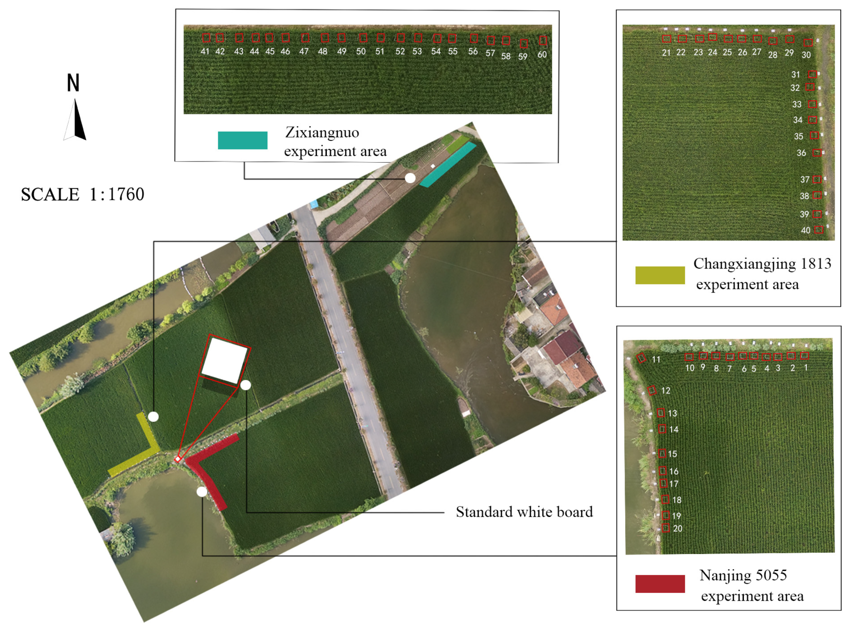
2.1. Field Experiment

The rice field experiment was conducted at Taiping Village, Qixia District, Nanjing (E119°16′18″, N32°20′47″). Located in the lower reaches of the Yangtze River, Nanjing has a typical north subtropical temperate climate with four distinct seasons, sufficient rainfall, abundant sunshine, 2100 h of sunshine per year, an average annual temperature of 15.4 °C, a frost-free period of 237 d, and an average annual precipitation of about 1100 mm. Such an excellent climate, with abundant rainfall and sunshine, provides a warm and humid growing environment for the experimental rice varieties. With flat and continuous arable lands, the agricultural cropping of this area is one crop per annum. The three rice varieties tested were Nanjing 5055, Changxiangjing 1813, and Zixiangnuo. In this experiment, a randomized block design was used, in which 20 test plots were set up for each variety with a plot area of 0.5 × 0.5 m; 10 rice plants were selected from each plot, with a total of 60 test plots, marked with numbers 1–60, respectively. This UAV observation experiment was conducted from 11 September 2022 to 2 October 2022, during which multispectral RS information of the rice canopy at the rice heading stage in each region was collected continuously. The collection was suspended in rainy weather. The stems and panicles started to grow on 11 September; panicle differentiation was completed on 2 October. The data in a total of 12 periods were collected. The rice experiment area is shown in Figure 1. Meanwhile, to determine the correlation of canopy spectral information with a rice heading rate and other indices, RS images were collected to conduct field sampling experiments synchronously. In this experiment, rice data of three varieties were collected, one plot for each variety, and 20 sampling spots were randomly selected in each plot. In addition, 10 rice plants were selected as the ROI in each sampling spot, and the rice heading in each ROI was measured by the counting method. The average heading rate of 20 sampling spots was taken as the rice heading rate in the plot on that day.

2.2. Acquisition and Pre-Processing of UAV Image Data

2.2.1. Acquisition of UAV Image Data

The multispectral RS images were acquired using DJI Phantom 4-M (P4M), a small multi-rotor, high-precision, aerial survey UAV produced by DJI. It was equipped with a multispectral camera with six 1-inch, 2.08 million pixel CMOS, including one color sensor for visible imaging and five monochrome sensors for multispectral imaging, in which multispectral imaging covered 450, 560, 650, 730, and 840 nm spectral bands. The multispectral image acquisition time was 10 a.m.–12 p.m. (noon) every day with clear and cloudless or less cloudy weather and an open field of view. The P4M supporting software DJI GS Pro V2.0.17 was used in the experiment for mapping selection. The UAV flew according to the route trajectory automatically planned by the flight control system, with a flight height of 12 m, set speed of 5 m/s, forward overlap of 80%, side overlap of 70%, its lens vertically downward, and an image resolution of 1600 × 1300 pixel. The ground sampling distance (GSD) was 0.63 cm/pixel. Meanwhile, a standard white board was placed in the experiment area. The size of the standard white board was 1 × 1m and made of PTFE material. The diffuse reflection rate can be regarded as a fixed value, convenient for subsequent radiation correction of the acquired image and elimination of the sunshine difference. The UAV RS experiment is shown in Figure 2.

2.2.2. Pre-Processing of Multispectral Data

Sixty groups of data were collected each day, and a total of 720 groups of multispectral aerial raw images were obtained. The raw images were recorded as TIF, which recorded a digital number (DN) and needed to be converted to reflectance data. The collected rice canopy multispectral data were pre-processed by concatenation correction, radiometric correction, etc., and square selection was delineated as regions of interest (ROI) at the center of the experimental plot, with a size of 50 × 50 pixels of each square selection [23]. For the images acquired each day, 20 ROIs were cropped out for each variety of rice, and the average value of pixels in each ROI was taken as the spectral value of that region. At the same time, the white correction area of the standard white board was selected. The spectral mean of the white correction area was taken to perform a band operation on the RS images. The calculation method is shown in Equation (1).
C I = I B W B ,
where CI is the spectral reflectance after radiation correction, I denotes the spectral mean of ROI in that band, W denotes the spectral mean of the standard white correction area in that band on that day, and B denotes the pixel mean in that band when the UAV lens is covered on that day.

2.3. Selection of VIs

VIs are indices composed of linear or nonlinear combinations between different bands, which can be used to diagnose the vegetation growth state or obtain various vegetation parameters by inversion. Currently, research results of UI have been achieved in the inversion studies of crop LAI, chlorophyll content, yield, etc. For this paper, 10 commonly used VIs were selected, with the specific calculation expressions and sources shown in Table 1.
In the subsequent model evaluation, the accuracy of the prediction model was evaluated using the fitting coefficient of determination (R2) and root mean square error (RMSE) of the measured and predicted values, with the calculation formula as follows:
R 2 = i = 1 n ( y i ^ y ¯ ) 2 i = 1 n ( y i ^ y ¯ ) 2 ,
RMSE = i = 1 n ( y i ^ y i ) 2 n ,
where y i ^ denotes the predicted value, y i denotes the measured value, y ¯ denotes the mean value, and n denotes the number of samples. The larger the coefficient of determination (R2) is, the smaller the root mean square error (RMSE) and the higher the model accuracy are.

2.4. Data Processing Methods

2.4.1. NN and SVR

With features such as nonlinear mapping and adaptive learning, NN can implement arbitrary nonlinear mapping of input and output data and adjust the connection weights between the connected input and output data by error back propagation to obtain a good fit. SVR is a supervised machine learning algorithm developed based on the theory of structural risk minimization. SVR implements nonlinear mapping to a high-dimensional space through a kernel function that transforms nonlinear processes in low dimensions into linear processes in high dimensions and finally solves the maximum marginal hyperplane (MMH) issue.

2.4.2. RF

RF is a machine learning model that integrates multiple regression and classification tree algorithms; it has the advantages of a great generalization capacity, fast training, and high accuracy. The RF regression model consists of multiple regression trees, and its output is the mean of the predictions of all decision trees. Based on the idea of bagging, the algorithm performs random sampling of the data set using the bootstrap sampling method. A total of two-thirds of the training samples are used to obtain the regression results; the remaining samples are used as the validation set to test the prediction accuracy of the model.

2.4.3. GBDT

GBDT regression is an iterative decision tree algorithm consisting of multiple decision trees. Based on the boosting iteration idea, the algorithm first initializes a weak model and proceeds towards the goal of reducing the residuals of the previous weak model in each subsequent round of iteration. Aiming at minimizing the loss function of the current learner, the GBDT model ultimately sums the results of all trained regression trees to obtain the final prediction results.

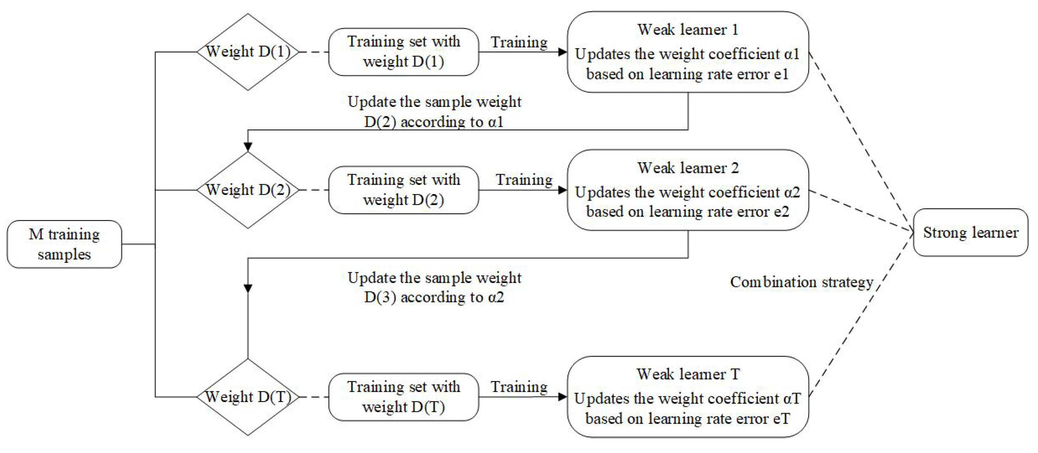
2.4.4. AdaBoost Algorithm

AdaBoost is an ensemble learning algorithm. Starting with a weak learning algorithm, its core idea is to obtain a series of weak learners through repeated training and build a strong learner with these weak ones by weighted voting [34]. Its regression steps are shown in Figure 3.

2.5. Data Strategy Analysis

In the experiment, the statistics of three rice varieties were collected, and the statistics of the heading rate were collected by a counting method in the experimental plot. When all rice varieties’ ears were out completely, within a certain sampling point, “A” represented the maximum of the collected ear emergence number in a test day, and “a” represented the ear emergence number collected every day. The daily rate of ear emergence of rice in this region can be calculated by the following formula:
X = a A
The average heading rate of 20 sampling points was taken as the rice heading rate of this day in this plot.
Meanwhile, a total of 720 sets of multispectral statistics were obtained in the experiment, among which 600 sets of statistics were randomly selected as training statistics and 120 sets of statistics were selected as test data. Using the method mentioned in Section 2.4, the reflectance value of each band of the rice canopy spectrum, single vegetation index, and multi-vegetation index were respectively taken as input statistics of the model, and the heading rate was taken as output statistics. With the determination coefficient (R2) and root mean square error (RMSE) as the discrimination criteria, the optimal model was selected to obtain the heading situation of rice at the heading stage.

3. Research Results

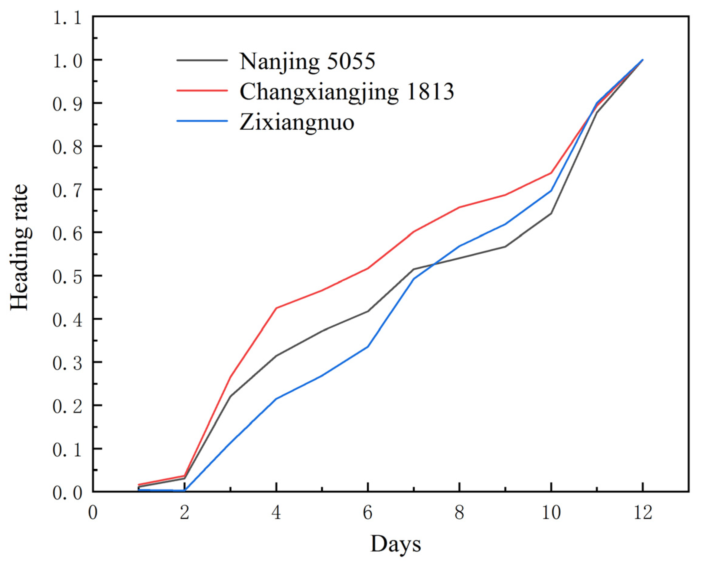
3.1. Rice Heading Rate

The whole growth process of rice is divided into six stages: tillering stage, nodulation stage, jointing stage, heading stage, grain filling stage, and maturity stage. The optimal period to control pests and diseases such as panicle blast is from the panicle opening/heading stage to the full heading stage (heading rate up to 80%), and the whole cycle lasts about 20 days. The different phases of the rice heading stage are shown in Figure 4.
The variation of rice heading rates over time is shown in Figure 5.
Figure 5 indicates that each variety of rice has a similar variation trend of heading rates but slightly different heading speeds. Changxiangjing 1813 showed rapid growth at 1–4 d, with the heading rate increasing rapidly from 0 to 42% before it slowed down and then increasing from 42 to 73% at 4–10 d. Nanjing 5055 showed a uniform heading rate at 1–7 d, with the heading rate varying from 0 to 51%, slowing down in the following 2 days, and increasing slowly from 51 to 56%. Although Zixiangnuo grew quickly in the heading rate at 6–7 d and 10–11 d, its overall heading rate was relatively uniform at the heading stage. In the last 2 days, the heading rates of the above three rice varieties showed accelerated increase by 27, 31, and 36%, respectively.

3.2. Spectral Reflectance

The multispectral RS test method for the rice canopy and the multispectral RS image processing and spectral reflectance extraction method described in Section 2.2.2 were used to obtain the spectral reflectance of three rice varieties (Nanjing 5055, Changxiangjing 1813, and Zixiangnuo) at five bands from 11 September 2022 to 2 October 2022, as detailed in Table 2.
As shown in Table 2, the spectral reflectance at the 840 and 730 nm bands was relatively high, fluctuating around 50 and 40%, respectively; the variation trends at the five bands were almost identical. In the first 5 days of the observation period, the spectral reflectance of the three rice varieties at all bands presented an upward trend, while, in the last 2 days of the observation period, the spectral reflectance at each band presented a downward trend. Nanjing 5055 and Zixiangnuo showed similar variation trends at all bands; the spectral reflectance of Changxiangjing 1813 varied in individual days and fluctuated sharply in the middle of the observation period.

3.3. Regression Models of Different Bands, Different VIs, and Heading Rates

For this paper, the multispectral information of the rice canopy at the heading stage was collected by a UAV equipped with a multispectral camera, and the rice heading rate in each plot was measured by the counting method at the same time. The VI was obtained by band combination operation, and regression analysis was performed on the variables using the traditional algorithms (NN, SVR, RF, GBDT, and AdaBoost) with the reflectance and VI of each band as the model input data and the heading rate as the output data, respectively. A total of 720 groups of data were collected in this experiment; 600 groups of data were randomly selected as the training data, and the remaining 120 groups of data were selected as the test data of the model.

3.3.1. Regression Models of Rice Canopy Spectral Information and Heading Rates at Different Bands

From the fitting effect of each band, the 650 and 730 nm bands had a relatively good fit, in which the 730 nm band had the best fit, with the highest coefficient of determination (R2) up to 0.79, corresponding to a good correlation between the model input and output variables; the model had a good prediction effect. The fitting effects of the 450, 560, and 840 nm bands were slightly inferior, and most of the fitting correlation coefficients for the heading rate were below 0.5, in which the 450 nm band had the worst fitting effect and the lowest fitting coefficient of only 0.31; the model had a relatively poor prediction effect. From the regression results of each band, the two red-edge bands had the best regression effects on the heading rate. This is because rice panicles are yellow at the heading stage, making it possible to distinguish yellow panicles from green leaves by color as the heading proportion increases. Thus, the rice was more sensitive to changes at the 650 and 730 bands at the heading stage. Hence, variables related to the 650 and 730 nm bands can be selected as input variables for the model in subsequent studies.
As shown in Table 3, from the regression methods, RF, GBDT, and AdaBoost all had relatively good regression effects and the overall RMSE was also small. Although NN showed a good fit at some bands, the fitting effect fluctuated significantly among the bands in general and the RMSE was slightly higher than the other methods, indicating that the NN model was more unstable than the other models. The RF fitting effect was relatively stable, and the fitting results were in the middle level of the regression methods. The SVR fitting effect was the worst, with the coefficient of determination generally lower than the other regression methods and the highest RMSE.

3.3.2. Regression Modes of Rice Single VIs and Heading Rate

Six VIs with high correlation with the 650 and 730 nm bands were selected: NDVI, GNDVI, NDRE, MNVI, CIred edge, and DVI. Regression analysis models of the heading rates were established using the above regression methods, respectively. The results are shown in Table 4.
As shown in Table 4, from the regression methods, SVR showed a good fit, with the coefficients of determination mostly above 0.6; however, its RMSE was generally higher than the other four methods, with instability in the regression of VI and heading rate. RF and GBDT had good fitting effects, with strong inversion capacity of the model. NN showed the worst comprehensive fitting effect. The AdaBoost algorithm based on ensemble learning had the best fitting effect of the VIs and heading rate, with the highest fitting coefficient of determination (R2) of 0.83. This is because AdaBoost can improve the feature extraction capacity of the model by building multiple regression models and assigning different weights to them.
From the VIs, NDVI had the best fitting effect. Except for NN (0.59), the fitting coefficients of determination of the other four methods were all above 0.7, which was evidently better than the other VIs; at this point, the model had a good prediction effect. In addition, GNDVI, MNVI, and NDRE also presented good fitting effects, indicating that these four VIs can be used for the prediction of a rice heading rate. The coefficients of determination of CIred edge and DVI were mostly around 0.4 based on each regression method, and the inverse performance of these two indices was insufficient for the prediction of heading rates.
In brief, rice heading rates can be properly predicted by using four VIs (NDVI, GNDVI, MNVI, and NDRE) through the regression analysis of data based on AdaBoost, and the model had a significant inversion capacity.

3.3.3. Regression Models of Rice Heading Rate Based on Multi-VIs

To determine the significance of monitoring rice heading rates, multi-VIs were input into different monitoring models. Based on four VIs (NDVI, GNDVI, MNVI, and NDRE), the inversion model of the rice heading rate was constructed by five methods (NN, SVR, RF, GBDT, and AdaBoost). In addition, the model parameters were adjusted to identify the optimal model.
Table 5 indicates that, for the inversion models of heading rates based on four VIs, the coefficients of determination (R2) of all five models were above 0.79, indicating a good prediction capacity. Compared with the traditional methods, the ensemble learning-based RF, GBDT, and AdaBoost showed good inversion capacity because the ensemble learning algorithm increased the generalization capacity of the model by homogenizing the bias. Combined with the two evaluation indices (R2 and RMSE), the AdaBoost model was the optimal model, with the coefficient of determination (R2) of 0.94 and RMSE of 0.12. Compared with the optimal model fitted by single-band and single VI, the coefficient of determination (R2) was increased by 0.15 and 0.11, respectively; RMSE was decreased by 0.08 and 0.07, respectively, indicating that the multi-VI inversion performance of heading rates can improve the prediction accuracy and robustness of the model. Hence, AdaBoost based on ensemble learning had better inversion capacity for the rice heading rate, which can provide a temporal reference for panicle blast control and plant protection operations around the heading stage. The inversion results of the optimal model are shown in Figure S1 of the Supplementary Material.

4. Discussion

In recent years, UAV-based multispectral RS technology has been increasingly used for monitoring the growth status and physiological indices such as nitrogen content, chlorophyll content, LAI, and yield of crops. It has made up for the defect of RS technology in crop monitoring with a single data type [35,36] and improved the accuracy and stability of crop growth information and physiological index estimation. In this paper, the spectral information of the rice canopy at the heading stage was continuously collected using UAV RS technology. Combined with the spectral reflectance and VI at different bands, inversion models of heading rates were established based on five algorithms (NN, SVR, RF, GBDT, and AdaBoost). The rice heading rate estimated based on the AdaBoost algorithm was the optimal model to acquire an accurate rice heading situation, which preliminarily verified the significant role of UAV multispectral RS in the unified control of rice panicle blast.
The three rice varieties tested in this study all fall into early-maturing late japonica rice, which is a common rice cultivar in the regions south of the Yangtze River in China. Previous studies indicated that, at the heading stage, rice panicles gradually grow and cover the whole canopy, resulting in differences in the growth status of each rice variety [37], as manifested by differences in physiological indices such as the heading rate and spectral reflectance. However, the area selected for this experiment has the same spatial and temporal dimensions, where the environmental variables such as light intensity, sunshine duration, and rainfall amount are almost identical. In the short-term continuous monitoring, it can be seen from the results of Figure 5 and Table 2 that indicators such as heading rate and spectral reflectance did not show significant differences. From this experiment alone, the intrinsic physiological properties of each rice variety are the most important factors affecting the heading rate and spectral reflectance of the canopy. This research lacked the investigation and analysis of intrinsic factors of each rice variety. In future studies, quantitative measurements of the rice heading rates of different varieties in different planting regions can be made to develop applicable strategies of plant protection operations for panicle blast control of different varieties in different regions.
This study indicated that, among the five spectral bands, the best fitting regression models for the heading rate were established at the 650 and 730 nm bands, suggesting that the red-edge band was more associated with the growth status of rice at the heading stage. This corroborated the studies by Miao et al. [38] and Yang et al. [39], which screened six VIs with high correlation with the red-edge band. Among them, NDVI, GNDVI, MNVI, and NDRE had better fit and prediction effects than the single band, indicating that the growth status of rice at the heading stage could be better characterized based on these four VIs, which was also verified by the final inversion model of the heading rate based on four VIs. The prediction analysis of the models showed that the estimation results based on various algorithms differed significantly, and the traditional machine learning methods could not estimate the rice heading rate effectively by using spectral information. The AdaBoost regression based on ensemble learning could predict the heading rate better than the other algorithms and was also more stable because the ensemble learning algorithm homogenized the bias and obtained better decision edges by weighting the edge components, which increased the generalization capacity of the model [40,41].
In this paper, we proposed a method to construct the inversion model of the rice heading rate by using UAV multispectral images and a multi-vegetation index, and the inversion results were good. The physiological state of rice at the heading stage can be determined based on this method, which provides theoretical support for pesticide precision spraying and intelligent plant protection machinery operation in rice panicle blast prevention and control. In the future, we will further set up more dispersed experimental areas and more diversified rice varieties’ experimental groups to perform a more detailed grading analysis. At the same time, this method can also be applied to other crops, so that more large areas of crop phenology and growth can be rapidly and accurately monitored.

5. Conclusions

  • The rice canopy color changed at the heading stage and further affected canopy reflectance. The fitting results of the regression models for single band and heading rate indicated that the 650 and 730 nm bands were more sensitive at the rice heading stage.
  • The inversion models of single band, single VI, multi-VIs, and multi-VI combinations were superior to the inversion models of single band and single VI. The AdaBoost-based inversion model of the rice heading rate was the best, with an R2 of 0.94 and RMSE of 0.12. Among the several methods, the ensemble learning-based algorithm could further improve the accuracy and robustness of the inversion model compared with the traditional machine learning algorithm.
The data acquisition and processing model established in this study can provide data support for the unified control of panicle blast and other pests during the heading period of rice.

Supplementary Materials

The following supporting information can be downloaded at: https://www.mdpi.com/article/10.3390/land12020469/s1, Figure S1: Best inversion model results.

Author Contributions

Conceptualization, C.C., G.C. and B.M.; methodology, B.M.; software, C.H. and B.M.; validation, C.H. and B.M.; data curation, B.M.; writing—original draft preparation, B.M.; writing—review and editing, C.C., G.C. and B.M.; visualization, C.H.; supervision, C.C.; project administration, G.C.; funding acquisition, G.C. and C.C. All authors have read and agreed to the published version of the manuscript.

Funding

This research was funded by a grant of the special funding for basic scientific research business expenses of central public welfare scientific research institutes (S202215).

Institutional Review Board Statement

Not applicable.

Informed Consent Statement

Not applicable.

Data Availability Statement

The data collected in this research are available when be required.

Conflicts of Interest

The authors declare no conflict of interest.

References

  1. Zahra, N.; Hafeez, M.B.; Nawaz, A.; Farooq, M. Rice production systems and grain quality. J. Cereal Sci. 2022, 105, 103463. [Google Scholar] [CrossRef]
  2. Huang, S.; Sun, C.; Qi, L.; Ma, X.; Wang, W. Rice panicle blast identification method based on deep convolution neural network. Trans. Chin. Soc. Agric. Eng. 2017, 33, 169–176. (In Chinese) [Google Scholar]
  3. Wen, X.; Xie, M.; Jiang, J.; Yang, B.; Shao, Y.; He, W.; Liu, L.; Zhao, Y. Advances in research on control method of rice blast. Chin. Agric. Sci. Bull. 2013, 29, 190–195. (In Chinese) [Google Scholar]
  4. Asibi, A.E.; Chai, Q.; Coulter, J.A. Rice Blast: A Disease with Implications for Global Food Security. Agronomy 2019, 9, 451. [Google Scholar] [CrossRef]
  5. Sriwanna, K. Weather-based rice blast disease forecasting. Comput. Electron. Agric. 2022, 193, 106658. [Google Scholar] [CrossRef]
  6. Feng, S.; Zhao, D.; Guan, Q.; Li, J.; Liu, Z.; Jin, Z.; Li, G.; Xu, T. A deep convolutional neural network-based wavelength selection method for spectral characteristics of rice blast disease. Comput. Electron. Agric. 2022, 199, 107199. [Google Scholar] [CrossRef]
  7. Kongcharoen, N.; Kaewsalong, N.; Dethoup, T. Efficacy of fungicides in controlling rice blast and dirty panicle diseases in Thailand. Sci. Rep. 2020, 10, 16233. [Google Scholar] [CrossRef]
  8. Du, Y.; Qi, Z.; Yu, J.; Yu, M.; Cao, H.; Zhang, R.; Yong, M.; Yin, X.; Pan, X.; Song, T.; et al. Effects of panicle development stage and temperature on rice panicle blast infection by Magnaporthe oryzae and visualization of its infection process. Plant Pathol. 2021, 70, 1436–1444. [Google Scholar] [CrossRef]
  9. Yang, G.; Liu, J.; Zhao, C.; Li, Z.; Huang, Y.; Yu, H.; Xu, B.; Yang, X.; Zhu, D.; Zhang, X.; et al. Unmanned Aerial Vehicle Remote Sensing for Field-Based Crop Phenotyping: Current Status and Perspectives. Front. Plant Sci. 2017, 8, 1111. [Google Scholar] [CrossRef]
  10. Zhang, J.; Tian, H.; Yang, J.; Pan, S. Improving Representation of Crop Growth and Yield in the Dynamic Land Ecosystem Model and Its Application to China. J. Adv. Model Earth Syst. 2018, 10, 1680–1707. [Google Scholar] [CrossRef]
  11. Hou, Y.; He, L.; Jin, N.; Zheng, C.; Liu, W.; Zhang, L. Establishment and application of crop growth simulating and monitoring system in China. Trans. Chin. Soc. Agric. Eng. 2018, 34, 165–175. (In Chinese) [Google Scholar]
  12. Duan, B.; Fang, S.; Gong, Y.; Peng, Y.; Wu, X.; Zhu, R. Remote estimation of grain yield based on UAV data in different rice cultivars under contrasting climatic zone. Field Crop. Res. 2021, 267, 108148. [Google Scholar] [CrossRef]
  13. Liu, T.; Zhang, H.; Wang, Z.; He, C.; Zhang, Q.; Jiao, Y. Estimation of the leaf area index and chlorophyll content of wheat using UAV multi-spectrum images. Trans. Chin. Soc. Agric. Eng. 2021, 37, 65–72. (In Chinese) [Google Scholar]
  14. Chen, Z.; Ren, J.; Tang, H.; Shi, Y.; Leng, P.; Liu, J.; Wang, L.; Wu, W.; Yao, Y.; Hasiyuya, P. Progress and perspectives on agricultural remote sensing research and applications in China. J. Remote Sens. 2016, 20, 748–767. (In Chinese) [Google Scholar]
  15. Liu, S.; Li, L.; Gao, W.; Zhang, Y.; Liu, Y.; Wang, S.; Lu, J. Diagnosis of nitrogen status in winter oilseed rape (Brassica napus L.) using in-situ hyperspectral data and unmanned aerial vehicle (UAV) multispectral images. Comput. Electron. Agric. 2018, 151, 185–195. [Google Scholar] [CrossRef]
  16. Aslan, M.F.; Durdu, A.; Sabanci, K.; Ropelewska, E.; Gültekin, S.S. A Comprehensive Survey of the Recent Studies with UAV for Precision Agriculture in Open Fields and Greenhouses. Appl. Sci. 2022, 12, 1047. [Google Scholar] [CrossRef]
  17. Li, S.; Yuan, F.; Ata-Ui-Karim, S.T.; Zheng, H.; Cheng, T.; Liu, X.; Tian, Y.; Zhu, Y.; Cao, W.; Cao, Q. Combining Color Indices and Textures of UAV-Based Digital Imagery for Rice LAI Estimation. Remote Sens. 2019, 11, 1763. [Google Scholar] [CrossRef]
  18. Ban, S.; Liu, W.; Tian, M.; Wang, Q.; Yuan, T.; Chang, Q.; Li, L. Rice Leaf Chlorophyll Content Estimation Using UAV-Based Spectral Images in Different Regions. Agronomy 2022, 12, 2832. [Google Scholar] [CrossRef]
  19. Colorado, J.D.; Cera-Bornacelli, N.; Caldas, J.S.; Petro, E.; Rebolledo, M.C.; Cuellar, D.; Calderon, F.; Mondragon, I.F.; Jaramillo-Botero, A. Estimation of Nitrogen in Rice Crops from UAV-Captured Images. Remote Sens. 2020, 12, 3396. [Google Scholar] [CrossRef]
  20. Jordan, M.I.; Mitchell, T.M. Machine learning: Trends, perspectives, and prospects. Science 2015, 349, 255–260. [Google Scholar] [CrossRef]
  21. Chen, C.; Cao, G.; Li, Y.; Liu, D.; Ma, B.; Zhang, J.; Li, L.; Hu, J. Research on Monitoring Methods for the Appropriate Rice Harvest Period Based on Multispectral Remote Sensing. Discrete Dyn. Nat. Soc. 2022, 2022, 1519667. [Google Scholar]
  22. Wan, L.; Cen, H.; Zhu, J.; Zhang, J.; Zhu, Y.; Sun, D.; Du, X.; Zhai, L.; Weng, H.; Li, Y.; et al. Grain yield prediction of rice using multi-temporal UAV-based RGB and multispectral images and model transfer—A case study of small farmlands in the South of China. Agric. For Meteorol. 2020, 291, 108096. [Google Scholar] [CrossRef]
  23. Xu, S.; Xu, X.; Blacker, C.; Gaulton, R.; Zhu, Q.; Yang, M.; Yang, G.; Zhang, J.; Yang, Y.; Yang, M.; et al. Estimation of Leaf Nitrogen Content in Rice Using Vegetation Indices and Feature Variable Optimization with Information Fusion of Multiple-Sensor Images from UAV. Remote Sens. 2023, 15, 854. [Google Scholar] [CrossRef]
  24. Tucker, C.J.; Elgin, J., Jr.; McMurtrey Iii, J.; Fan, C. Monitoring corn and soybean crop development with hand-held radiometer spectral data. Remote Sens. Environ. 1979, 8, 237–248. [Google Scholar] [CrossRef]
  25. Gitelson, A.A.; Kaufman, Y.J.; Merzlyak, M.N. Use of a green channel in remote sensing of global vegetation from EOS-MODIS. Remote Sens. Environ. 1996, 58, 289–298. [Google Scholar] [CrossRef]
  26. Daughtry, C.S.; Walthall, C.; Kim, M.; De Colstoun, E.B.; McMurtrey Iii, J. Estimating corn leaf chlorophyll concentration from leaf and canopy reflectance. Remote Sens. Environ. 2000, 74, 229–239. [Google Scholar] [CrossRef]
  27. Gong, P.; Pu, R.; Biging, G.S.; Larrieu, M.R. Estimation of forest leaf area index using vegetation indices derived from Hyperion hyperspectral data. IEEE Trans. Geosci. Electron. 2003, 41, 1355–1362. [Google Scholar] [CrossRef]
  28. Gitelson, A.A.; Kaufman, Y.J.; Stark, R.; Rundquist, D. Novel algorithms for remote estimation of vegetation fraction. Remote Sens. Environ. 2002, 80, 76–87. [Google Scholar] [CrossRef]
  29. Jordan, C.F. Derivation of leaf-area index from quality of light on the forest floor. Ecology 1969, 50, 663–666. [Google Scholar] [CrossRef]
  30. Broge, N.H.; Leblanc, E. Comparing prediction power and stability of broadband and hyperspectral vegetation indices for estimation of green leaf area index and canopy chlorophyll density. Remote Sens. Environ. 2001, 76, 156–172. [Google Scholar] [CrossRef]
  31. Birth, G.S.; McVey, G.R. Measuring the color of growing turf with a reflectance spectrophotometer 1. Agron. J. 1968, 60, 640–643. [Google Scholar] [CrossRef]
  32. Huete, A.; Didan, K.; Miura, T.; Rodriguez, E.P.; Gao, X.; Ferreira, L.G. Overview of the radiometric and biophysical performance of the MODIS vegetation indices. Remote Sens. Environ. 2002, 83, 195–213. [Google Scholar] [CrossRef]
  33. Roujean, J.-L.; Breon, F.-M. Estimating PAR absorbed by vegetation from bidirectional reflectance measurements. Remote Sens. Environ. 1995, 51, 375–384. [Google Scholar] [CrossRef]
  34. Cao, Y.; Miao, Q.; Liu, J.; Gao, L. Advance and prospects of AdaBoost algorithm. Acta Autom. Sin. 2013, 39, 745–758. (In Chinese) [Google Scholar] [CrossRef]
  35. Benami, E.; Jin, Z.; Carter, M.R.; Ghosh, A.; Hijmans, R.J.; Hobbs, A.; Kenduiywo, B.; Lobell, D.B. Uniting remote sensing, crop modelling and economics for agricultural risk management. Nat. Rev. Earth Env. 2021, 2, 140–159. [Google Scholar] [CrossRef]
  36. Orynbaikyzy, A.; Gessner, U.; Conrad, C. Crop type classification using a combination of optical and radar remote sensing data: A review. Int. J. Remote Sens. 2019, 40, 6553–6595. [Google Scholar] [CrossRef]
  37. Luo, S.; Jiang, X.; Jiao, W.; Yang, K.; Li, Y.; Fang, S. Remotely Sensed Prediction of Rice Yield at Different Growth Durations Using UAV Multispectral Imagery. Agriculture. 2022, 12, 1447. [Google Scholar] [CrossRef]
  38. Miao, X.; Miao, Y.; Liu, Y.; Tao, S.; Zheng, H.; Wang, J.; Wang, W.; Tang, Q. Measurement of nitrogen content in rice plant using near infrared spectroscopy combined with different PLS algorithms. Spectrochim Acta A Mol. Biomol. Spectrosc. 2023, 284, 121733. [Google Scholar] [CrossRef]
  39. Yang, F.; Fan, Y.; Li, J.; Qian, Y.; Wang, Y.; Zhang, J. Estimating LAI and CCD of rice and wheat using hyperspectral remote sensing data. Trans. Chin. Soc. Agric. Eng. 2010, 26, 237–243. (In Chinese) [Google Scholar]
  40. Ganaie, M.A.; Hu, M.; Malik, A.K.; Tanveer, M.; Suganthan, P.N. Ensemble deep learning: A review. Eng. Appl. Artif. Intel. 2022, 115, 105151. [Google Scholar] [CrossRef]
  41. Mohammed, A.; Kora, R. A Comprehensive Review on Ensemble Deep Learning: Opportunities and Challenges. J. King Saud. Univ. Com. 2023. [Google Scholar] [CrossRef]
Figure 1. Rice experiment area.
Land 12 00469 g001
Figure 2. (a) DJI Phantom 4-M (P4M); (b) rice RS multispectral information acquisition.
Land 12 00469 g002
Figure 3. Flow chart of AdaBoost algorithm.
Land 12 00469 g003
Figure 4. True color RGB and false color RGB images at different phases of the rice heading stage.
Land 12 00469 g004
Figure 5. Rice experiment area.
Land 12 00469 g005
Table 1. VI and calculation formula.
Vegetation IndexCalculation FormulaReference
Normalized Difference Vegetation Index
(NDVI)
(NIR − R)/(NIR + R)Tucker et al. [24]
Green Normalized Difference Vegetation Index
(GNDVI)
(R − G)/(R + G)Gitelson et al. [25]
Normalized Difference Red-Edge Index
(NDRE)
(NIR − RE)/(NIR + RE)Daughtry et al. [26]
Modified Nonlinear Vegetation Index
(MNVI)
1.5 (NIR2 − R)/(NIR2 + R + 0.5)Gong et al. [27]
Red-Edge Chlorophyll Index
(CIred edge)
NIR/RE − 1Gitelson et al. [28]
Difference Vegetation Index
(DVI)
NIR − RJordan. [29]
Triangular Vegetation Index
(TVI)
60(RE − G) − 100(R − G)Broge et al. [30]
Ratio Vegetation Index
(RVI)
NIR/RBirth et al. [31]
Enhanced Vegetation Index
(EVI)
2.5(NIR − R)/(NIR + 6NIR − 7.5B + 1)Huete et al. [32]
Optimized Soil Adjusted Vegetation Index
(OSAVI)
1.16(NIR − R)/(NIR + R + 0.16)Roujean et al. [33]
Note: R is red band, G is green band, B is blue band, RE is red-edge band, NIR is near infrared band.
Table 2. Average spectral reflectance in different bands during the experiment period.
DateVarietiesBand
450560650730840
11 September Nanjing 505527.03%26.15%17.92%38.65%48.52%
Changxiangjing 181331.84%33.28%26.15%43.15%50.14%
Zixiangnuo24.25%23.81%14.54%38.15%46.58%
12 SeptemberNanjing 505527.12%27.46%18.08%39.78%47.97%
Changxiangjing 181332.60%33.93%26.04%44.42%50.26%
Zixiangnuo24.66%23.67%15.02%39.27%46.74%
16 SeptemberNanjing 505529.26%29.19%21.08%41.23%50.75%
Changxiangjing 181335.45%34.16%27.48%47.28%55.67%
Zixiangnuo25.16%24.49%15.58%41.25%50.53%
17 SeptemberNanjing 505530.66%29.79%21.17%41.92%51.06%
Changxiangjing 181336.16%32.14%24.85%47.21%56.58%
Zixiangnuo25.78%25.47%14.99%42.82%51.37%
18 SeptemberNanjing 505528.86%28.83%21.00%38.84%54.32%
Changxiangjing 181340.04%36.14%30.44%47.12%63.43%
Zixiangnuo25.47%26.59%15.89%42.31%60.97%
19 SeptemberNanjing 505528.54%27.84%20.66%37.71%56.81%
Changxiangjing 181333.70%31.43%24.44%43.36%62.22%
Zixiangnuo21.78%23.06%13.62%38.70%56.24%
20 SeptemberNanjing 505527.22%27.34%19.78%35.98%47.68%
Changxiangjing 181337.56%34.06%28.78%42.23%53.42%
Zixiangnuo26.63%28.47%17.21%40.70%52.93%
21 SeptemberNanjing 505529.08%28.54%21.08%38.40%49.99%
Changxiangjing 181337.31%35.64%28.55%46.73%58.96%
Zixiangnuo26.08%29.98%16.71%48.36%57.62%
22 SeptemberNanjing 505525.90%25.94%18.56%34.83%46.33%
Changxiangjing 181336.04%33.74%25.96%46.25%56.84%
Zixiangnuo25.22%27.84%16.51%44.50%55.63%
25 SeptemberNanjing 505530.95%32.12%24.10%39.67%49.67%
Changxiangjing 181338.48%36.64%29.03%47.26%58.03%
Zixiangnuo24.28%25.66%16.35%41.90%58.73%
29 SeptemberNanjing 505531.94%33.29%25.80%41.90%54.78%
Changxiangjing 181336.58%35.02%28.40%46.84%64.04%
Zixiangnuo26.88%23.80%18.90%37.38%62.24%
2 OctoberNanjing 505527.79%28.19%20.98%39.87%46.93%
Changxiangjing 181331.10%30.79%25.01%41.41%49.71%
Zixiangnuo24.67%24.26%17.69%34.59%46.02%
Table 3. Fitting results of single-band information input model.
Input BandFitting ModelFitting Result
R2RMSE
450NN0.400.30
SVR0.310.30
RF0.520.28
GBDT0.590.24
AdaBoost0.630.27
560NN0.430.30
SVR0.330.35
RF0.530.27
GBDT0.510.34
AdaBoost0.650.18
650NN0.390.33
SVR0.400.33
RF0.670.34
GBDT0.630.37
AdaBoost0.720.29
730NN0.680.27
SVR0.510.25
RF0.630.21
GBDT0.660.18
AdaBoost0.790.20
840NN0.360.26
SVR0.560.29
RF0.430.24
GBDT0.480.21
AdaBoost0.530.17
Table 4. Fitting effect of single VI and heading rate.
Input VIFitting ModelFitting Result
R2RMSE
NDVINN0.590.31
SVR0.760.32
RF0.700.29
GBDT0.750.22
AdaBoost0.830.19
GNDVINN0.410.33
SVR0.600.31
RF0.440.27
GBDT0.510.41
AdaBoost0.540.37
NDRENN0.250.24
SVR0.430.26
RF0.390.25
GBDT0.520.19
AdaBoost0.640.11
MNVINN0.520.26
SVR0.610.28
RF0.470.27
GBDT0.440.35
AdaBoost0.630.30
CIred edgeNN0.340.26
SVR0.420.29
RF0.390.25
GBDT0.460.28
AdaBoost0.410.37
DVINN0.270.19
SVR0.350.30
RF0.540.24
GBDT0.510.33
AdaBoost0.630.31
Table 5. Inversion results based on four VIs and heading rate.
Fitting ModelFitting Result
R2RMSE
NN0.810.17
SVR0.790.15
RF0.890.33
GBDT0.910.25
AdaBoost0.940.12
Disclaimer/Publisher’s Note: The statements, opinions and data contained in all publications are solely those of the individual author(s) and contributor(s) and not of MDPI and/or the editor(s). MDPI and/or the editor(s) disclaim responsibility for any injury to people or property resulting from any ideas, methods, instructions or products referred to in the content.

