Abstract
Conversion rule is a key element for a cellular automata (CA) model, and it is a significant and challenging issue for both domestic and international experts. Traditional research regarding CA models often constructs a single conversion rule for the entire study area, without differentiating it on the basis of the unique growth features of each location. On the basis of this, a partitioned and heterogeneous land-use simulation model (PHLUS) is constructed by integrating a CA and Markov model: (1) A general conversion rule is constructed for the entire study area. By establishing a land development potential evaluation index system, the conversion rule is refined and differentiated; (2) By coupling a CA model with a Markov model, PHLUS can realize land-use simulation both in micro and macro scales. A simulation study is conducted for the Pearl River Delta region. The results show that: (1) By transforming the CA model rules to further distinguish zones, the accuracy is improved. Compared with the traditional CA-Markov model, the simulation accuracies for 2010 and 2020 are improved by 11.55% and 7.14%, respectively. For built-up land simulation, the PHLUS simulation errors for 2010 and 2020 are only 0.7% and 0.57%, respectively; and (2) Under land-use simulation for 2030, cultivated land and forest land will transfer to built-up land. The built-up land area will reach 10,919 km2. Guangzhou and Shenzhen have the greatest potential for land development, and the built-up land area for the two cities will reach 2727 km2.
1. Introduction
China is currently urbanizing at an unprecedented rate, with cities quickly increasing in number and size. Chain reactions have led to an increase in human alteration of the environment and resource exploitation, as well as the encroachment of metropolitan areas over vast tracts of agricultural and forest land, which has resulted in a variety of ecological issues. The loss of vegetation caused by urbanization affects regional carbon storage and carbon balance, reduces the capacity of freshwater supply, leads to a reduction in biological habitats, is detrimental to the development of regional biodiversity, and causes damage to regional ecosystems [1,2]. One of the main causes of farmland loss is urban growth, and as a result of this sharp fall in farmland, the problem of the nation’s food supply and food security has gained a great deal of attention [3,4]. The resolution of the aforementioned issues is aided by modeling and predictions of land-use change. Land-use change modeling is a quantitative description and representation of land-use change in the studied region, and it can give a scientific basis for national decisions regarding ecological risk assessment, land planning, and management, among other things. Land-use change is a core area of ecological research, and scholars at home and abroad have been investigating a range of methods and models for making accurate predictions of future land-use change. Since 1979, when the cellular automata (CA) model was first applied to geographic research by Tobler [5], it has been widely used in modeling land-use change because of its powerful computational properties and its ability to solve complex system problems through microsystems [6,7]. The Markov model can quantify and simulate the transition states between different land-use types and obtain the probability of transition between different land-use types [8]. The Markov model has been widely used in land-use simulation in recent years [9,10,11].
Due to the complexity of land-use change, it is frequently difficult to represent and predict land-use change in all aspects when using a single model in land-use prediction research. Therefore, to study land-use change and dynamic properties, researchers frequently pair various models. The integration of a CA model with Markov models [12,13,14], CA model with statistical models [15,16], a system dynamics (SD) model with statistical models [17], and economic and statistical models have been widely used in land-use change research [18]. Therefore, researchers often couple multiple models to study land-use change and dynamic characteristics. Among the commonly used CA models, the Logistic-CA model uses a logistic function to construct a relationship between land-use change and drivers by normalizing the dependent variables [19,20]. However, as a linear fitting model, the Logistic-CA model cannot express the land-use change nonlinear characteristics [21]. The coupled artificial neural network (ANN) model with CA model has a strong self-learning capability and is advantageous in simulating urban sprawl [22,23]. However, it has difficulties in correctly parameterizing and optimizing the configuration for land-use change [24,25,26]. The coupled SD model with CA model can simulate land-use change both on macro and micro scales [27,28,29]. However, based on SD model features, complex causality diagrams needs to be built [29]. The CA-Markov model combines the ability of the CA model to simulate spatial changes in complex systems with the advantages of the Markov model for long-term prediction. It not only improves the prediction accuracy of land use type transformation but also can effectively simulate the spatial changes of land use patterns [30]. It has greater scientific bearing and practicality and can simulate and predict land use changes more accurately [8].
One of the fundamental ideas of the CA model is the transition rule, and how it is defined has received a great deal of attention and study [31]. The transition rule is the notion that the state of the cell at a given moment depends on the state of the cell at that moment and the state of the neighboring cells. Even yet, the CA-Markov model overcomes the drawbacks of the single model and offers the benefits listed in the previous section. However, the traditional meta-cellular automata model uses a uniform transformation rule for evolution. The actual land-use status and the natural environment and socio-economic conditions behind it are highly heterogeneous [32,33]. This approach tends to ignore the spatial and temporal variability in the evolution of geographical phenomena and the spatial heterogeneity of evolutionary patterns.
This research proposes a partitioned and heterogeneous CA-Markov model for the simulation and prediction of land-use change to address this problem. The process of comprehensively evaluating or grading a piece of land’s natural, economic, and productive potential by its intended use is known as the evaluation of land development potential. A better way to address the issue of low modeling accuracy for land-use change due to spatial heterogeneity is to partition according to land development potential. Different levels of land development potential can result in different levels of land-use change. While taking into consideration spatial heterogeneity, there is some consistency within the established limits of the same area, and additional refinement still permits localized variability. Local adaption rules were chosen to be produced in many sorts of local regions, according to their features and under the condition that the general premise is satisfied, to make the constructed model more practical and scientific. The simulation results for PHLUS were validated using land-use data from 2000 to 2020. The validated PHLUS model is used to forecast the land-use change in the PRD region from 2020 to 2030, to further explore the future land-use pattern and the factors behind it that promote land-use change and to provide theoretical research support for the state and relevant departments to formulate refined land-use proposals.
2. Materials and Methods
2.1. Study Area
The Pearl River Delta is located in the south–central part of Guangdong Province, China. The administrative division includes the nine cities of Guangzhou, Foshan, Zhaoqing, Shenzhen, Dongguan, Huizhou, Zhuhai, Zhongshan, and Jiangmen (Figure 1). By 2020, the combined GDP of the nine PRD cities reached RMB 8946.988 billion, accounting for approximately 8.8% of the national GDP (NBSC, 2021). The total population of the PRD region is 78,235,400, accounting for approximately 61.97% of the total population of Guangdong Province (Guangdong Statistical Yearbook, 2021). The total administrative area of the PRD region is approximately 54,000 square kilometers, and the land-use structure is mainly non-built-up land, which accounts for approximately 84% of the total area. Since the reform and opening up, the Pearl River Delta (PRD) region has seen rapid economic development and has become one of the most important economic hub regions in China.
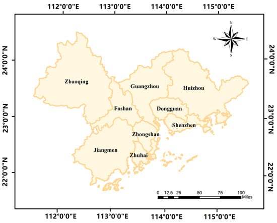
Figure 1.
The study area location.
With the expansion of the Pearl River Delta’s economic takeoff, the widespread expansion of urban land has significantly reduced available land resources. Additionally, the increase in population has resulted in enormous energy consumption and an inefficient industrial structure that has caused environmental challenges and a variety of land-use problems. First, the several areas to which some of the lands belong lead to a complicated relationship of the interests that they impact and is one of the issues that need to be addressed. Secondly, the lack of comprehensiveness in the development and construction of the land leads to a more complex geographical landscape pattern. The last is the inefficient use of land and the lack of rationalization of the different land-use types. Therefore, it is urgent to pay attention to how to promote efficient and rational land-use change and ecologically sustainable development in the PRD region.
2.2. Data Source and Processing
On the basis of the data availability and accessibility, the PRD region’s land-use statistics for the years 2000, 2010, and 2020 were used for modeling and forecasting. The choice of 10 years as the time interval is scientific. If the time interval is too short, there are problems, such as land-use changes not being obvious, wherein the results are not easily observed; if the period is too large, the variability of uncertainty is greater, and the time sensitivity and information are lower [34]. Moreover, according to the land change in the Pearl River Delta from 2000 to 2020, the expansion of urban land is more rapid after 2010, which serves as a turning point; in addition, China has to achieve the peak of carbon emissions by 2030, so it is of great significance by predicting its land-use change. The Data Centre for Resources and Environmental Sciences, Chinese Academy of Sciences, has contributed the land-use data, which are based on Landsat TM images with a spatial resolution of 1000 m [35]. The accuracy was checked through field surveys and random sampling according to the proportion of 10% of the number of counties. These land use data are evaluated with a combined precision of more than 94.3% [36]. The land-use data are broken down into five categories—cultivated land, woodland, grassland, water, and built-up land—to render the simulation results more understandable and to make the model simpler [37]. Among them, in the Pearl River Delta region, the unused land is too small and distributed mainly inside the construction land, which has little impact on the land-use prediction results. Therefore, the unused land is regarded as construction land for research purposes [38]. As one of the most typical areas of urbanization, the Pearl River Delta region has the most significant changes in built-up land, so the simulation and prediction of built-up land is the focus of this research.
Land-use change is influenced by a variety of drivers, each of which has a different impact on different land-use types of change. Road networks can undertake to connect traffic and enable inter-regional mobility accessibility. It has a great impact on regional development and is an important driver of land-use change [39,40,41]. Distance to highways, national highways, and railroads have often been considered important drivers of land-use change in recent studies [42,43,44,45]. A station plays the role of not only a transportation hub but also a place where numerous human activities take place. It can play a role in influencing the surrounding space as well as changing the type of land use, especially the area of built-up land [39]. On the other hand, areas for human activities, such as recreation centers, tourist attractions, and restaurants are considered to be important drivers of land-use type change [40].
DEM data, slope data, river data, precipitation data, road data, point of information (POI) data, population density data, nighttime light intensity data, and GDP data were used in this study (Table 1). To unify the controllable factors and improve the reliability of the comparison study, the coordinate system for all spatial data was defined as WGS_1984_PDC_Mercator. The DEM data were provided by the Data Center for Resources and Environmental Sciences, Chinese Academy of Sciences and were generated on the basis of the latest resampling of SRTM V4.1 data with a spatial resolution of 250 m. Slope data were generated by extracting DEM data with a spatial resolution of 250 m. Road data were obtained from OpenStreetMap download and cropped to generate the portion of the data. The POI data for this study were sourced from Baidu Maps, specifically referring to points on the map that do not have geographical significance but have other meanings. In this paper, four types of POIs were captured from the map: restaurants, markets, traffic stations, and scenic spots, with the aim of studying the impact of socio-economic factors on land-use change. To assess the influence of environmental factors on land-use change, distance to highways, distance to national roads, distance to provincial roads, distance to railways, distance to tourist attractions, distance to restaurants, distance to supermarkets, distance to transport stations, and distance to rivers were used as influencing factors (Figure 2). In addition, GDP and population data were obtained through the China Statistical Yearbook and the Guangdong Statistical Yearbook in aggregate, among others.

Table 1.
Data used in the study.
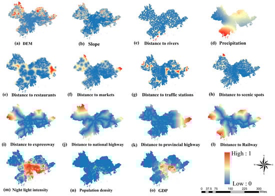
Figure 2.
Spatial variables in Pearl River Delta. (a–d) show the natural factors. (e–o) show the social and economic factors (All the data were normalized).
2.3. Methods
2.3.1. Overall Framework of the PHLUS Model
We first established a land use potential evaluation index system for the study area. Based on the evaluation results, the study area was zoned. Global conversion rules and local conversion rules were obtained by combining different land use drivers. The MCE criterion was used to obtain the land use suitability atlas. The land use transfer matrix was obtained by combining the Markov model. Finally, the coupled CA model and Markov model were iterated to simulate and predict the land use. The overall framework is shown in Figure 3.
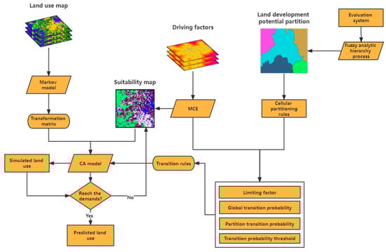
Figure 3.
The framework for PHLUS.
2.3.2. Establishment of the Evaluation System
The construction of a reasonable evaluation index system is an important basis for land-use zoning, and the selection of evaluation indexes is the key to the construction of the evaluation system. This paper is based on the principles of comprehensiveness, representativeness, science, and availability of data in the selection of evaluation indicators. In the context of present-day land-use change, the research object is split into three layers: these are the target level, the guideline level, and the indicator level. The target tier was chosen to evaluate the development potential of the land, which is key to the realization of the land-intensive use model. The assessment of land development potential helps the country to optimize the land structure and layout of the region. The potential of the economic supply of urban land resources is fully exploited to achieve the best urban land input–output ratio and land utilization rate, which is, therefore, used as the objective of the FAHP model. The natural ecological potential, the socio-economic potential, and the spatial structural potential were selected as the three first-level indicators, i.e., the guideline layer. The secondary indicator layers derived from the primary indicators are collectively referred to as the criteria layers. For example, there are direct effects of elevation and slope on the choice of industrial location, urban development, and land-use type changes. The elevation and slope factors were, therefore, selected for this study to characterize the role of natural condition excellence in the development potential of the land. The composition of land types, ecological controls, geological hazards, and ground subsidence was selected to measure the level of the ecological sensitivity of the study area. At the same time, population density is used to characterize the amount of land demanded by the population and the level of development support. GDP per capita and the proportion of output value of secondary and tertiary industries reflect the regional industrial structure, the level of economic development, and the size of economic demand for land, while the proportion of land for construction reflects the potential for urbanization and, thus, represents the economic development potential of land development. The current spatial pattern of land-use change is used as a basis for land redevelopment. The study examines the spatial pattern of land in terms of dominance, distance, and agglomeration. Land class dominance, nearest distance, land agglomeration, and high- and low-value agglomeration are selected to express the spatial structure potential of the land.
2.3.3. Determination of Evaluation Sets and Weights
The evaluation of future land-use development potential is the collection of all evaluation results for all the evaluation objects, i.e., in this study, the evaluation results were judged on a five-point scale, with the grading shown in the following equation. The specific grading evaluation criteria requirements draw on the table, which is realistically referable, drawing on the findings of industry experts and relevant empirical information.
where represent the four states of very high potential, high potential, medium–high potential, medium–low potential, and low potential for land-use development, respectively.
According to the degree of influence of each indicator in the evaluation index system on the development potential of land-use change, the judgment matrix is obtained by comparing the criterion layer with the indicator layer. The judgment matrix indicators are based on the scale of 1 to 9 proposed by Saaty. Then, on the basis of the judgment matrix established, the square root method is used to determine the maximum eigenvalue and the corresponding eigenvector of the judgment matrix of each layer of indicators. The eigenvectors are further normalized to obtain the weights of the factors in this layer relative to the corresponding factors in the previous layer. Finally, a consistency test is performed to ensure that the requested weights are assigned to reasonable reliability [46].
where CI is an indicator of consistency; is the maximum eigenvalue; m is the order of the judgment matrix; CR is the stochastic consistency ratio of the judgment matrix, such that when CR ≤ 0.1, the judgment matrix is consistent; and RI is the average random consistency indicator.
2.3.4. Determination of Membership Function
The determination of the degree of affiliation is a matter of judging individual indicators. The results of the indicator processing are divided into five levels of superiority and inferiority for the development of land development potential, in descending order of superiority and inferiority from to . In addition, the indicators were assigned [0.1, 0.9] using threshold-type and S-type affiliation functions, according to the types of indicators in Table 2. The land dominance, nearest proximity, high- and low-value clustering, land clustering, and population density are assigned using an S-type affiliation function, and modeling using existing metric systems and processing methods [47,48]. In this paper, we construct an evaluation system that integrates natural ecology, social economy, and spatial structure. We refer to the existing inter-district classification system and combine the characteristics of the study area PRD itself [49]. The fuzzy comprehensive evaluation method is used to classify 11 index values into 5 levels [50], and the intervals are classified in the software by the natural interruption method, as shown in Table 3. As economic development activities on the land are roughly inversely proportional to ecological sensitivity, the natural ecological factors are treated in reverse [49].
Table 2.
Description of evaluation index of land development potential.
Table 3.
Classification of land-use potential evaluation indexes.
Threshold-based affiliation functions:
S-affiliation function:
2.3.5. Fuzzy Comprehensive Evaluation Division
The comprehensive evaluation system for future land development potential consists of three tiers. Therefore, a two-level fuzzy integrated evaluation is carried out: the evaluation of the indicator level on the criterion level and the evaluation of the criterion level on the target level. Due to a large number of factors in the evaluation system, FAHP was used to make the judgment, and then the weighting was achieved through the sub-weights of each layer. The comprehensive discriminant index S is determined through the affiliation function and is calculated as shown in the formula below.
where is a synthetic operator, is a vector of factor weights, vector of representative factor weights, R is the judgment matrix, denotes the affiliation of factor (m = 1, 2, …, 14) to the rubric (n = 1, 2, 3, 4, 5), m is the number of corresponding factors (m = 14), and j is the level of classification (n = 5).
2.3.6. Heterogeneous Model
CA models contain numerous spatial variables in the simulation and prediction of land-use, and different transformation rules can lead to significant differences in the results obtained from CA models. The conversion rule, the core of the CA model, can reflect the state of land-use regarding numerous spatial variables. The determination of conversion rules is related to the probability of land-use conversion. The probability of land area conversion is influenced by a range of spatial variables. By deriving the probability of land-use conversion for different land-use types under the influence of regional environmental influences, a cellular conversion rule can be derived.
The transition probability of cellular is decomposed into two parts, the local transition probability and the global transition probability, which together determine the transition direction of that cellular, where the local conversion probability refers to the effect of the land-use condition around the cell to be evaluated on the cellular (evaluation of the neighboring states of cellular within a partition). At a given moment, it is only related to the state of all cells within a set detection window, independent of the spatial location of the cells. The global transition probability, on the other hand, refers to the effect on the cellular transition of a global factor that is constant or varies very little throughout the simulation.
Global transition probabilities assess the change in the state of cellular from the perspective of the region as a whole. It is determined by the various external conditions that influence the transformation of urban sites at the time of the simulation of the initial state. This study uses a multi-criteria evaluation (MCE) approach to influence the probability of conversion to a land-use type by varying the weights of a range of spatial variables. The probability of conversion can be expressed by the following equation:
where denotes the transition probability of the cellular at (i, j) under the kth partition at moment t; represents the suitability of the cellular state for transformation at location (i, j) at moment t; represents the maximum value of ; and represents the diffusion coefficient.
The suitability of the cell for state transfer is determined by several spatial variables [51]:
where denotes a spatial variable; denotes weight; and indicates a limiting factor, which takes the value of 0 when the cell is in the restricted development zone, and the value of 1, otherwise.
The model treats the neighborhood cell state as an important factor influencing the transition of this cell, and the local transition probability is determined by the neighborhood cell state [46]. The formula is expressed as:
where represents the local transition probability of the cell; z indicates the state of the target cell in the neighborhood; and n is the number of neighborhood cells.
Synthetic probability is a function of the superposition of global and local transition probabilities. The formula is expressed as:
By comparing the maximum value of the probability of each land-use type changing to another land-use type with the extracted threshold value, it is possible to determine whether the cellular has changed at a given point in time.
2.3.7. CA-Markov Model
CA models are discrete in time, space, and state and can be used to model the dynamics of complex systems as they evolve in time and space. The CA model includes the cellular, the cellular space, the neighborhood, and the rules. In land-use modeling, land-use data can be seen as consisting of numerous cellulars. Each cellular space has the property of its spatial location, and the cellular state is influenced by the state of neighboring cellular, and it changes according to certain transformation rules. The expression is:
where is a finite, discrete set of states of the cellular; represents the current moment and the next moment of the cellular; (Z) is the conversion rule for the cellular; and N is the cellular neighborhood.
A Markov process is a stochastic process in which the state of any moment in a finite sequence of times … and is related only to the state of its predecessor and not to the states of the other moments. In modeling prediction studies of land-use change, the process of land-use type change can be thought of as a Markov process. Interconversion between any two land-use types can occur over a longer time scale in a given region in a way that is influenced by the land-use type that precedes it [3]. Using the state shift probabilities in Markov models, it is possible to simulate the prediction of the amount or proportion of area where different land-use types switch to each other during land-use change. The formula utilized is shown below.
where and represent the land-use status at moments and , respectively, and is the state transfer matrix of the land-use change process, the formula of which is as follows.
3. Results
3.1. Results of the Geographical Partitioning of the Pearl River Delta Urban Agglomeration
First, each indicator of the future land development potential evaluation system was weighted and superimposed. Table 4 shows the results of the weights of each indicator. Then, the map algebra function of ArcGIS software was used to multiply the values of each indicator by the corresponding weights. Finally, the land development potential evaluation score of each region could be obtained (Figure 4). On the basis of the evaluation score, the land use development potential can be divided into five categories: very high potential area, high potential area, medium potential area, low potential area, and very low potential area. As the grade decreases, it is characterized by lower land development suitability, lower land economic benefits, lower ecological vulnerability, and higher ecological sensitivity (Table 5) [49].
Table 4.
Indicator weights results.
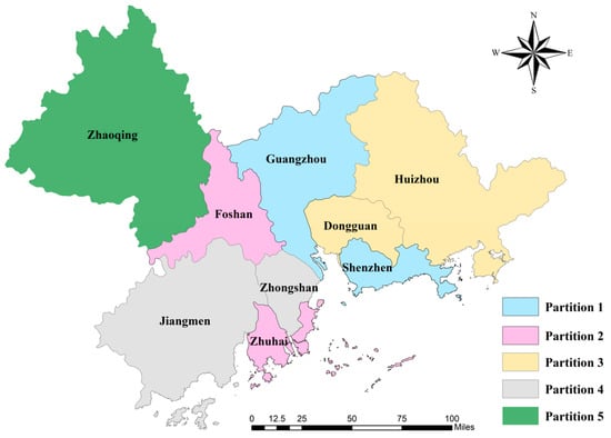
Figure 4.
The partition for Pearl River Delta.
Table 5.
Results of land development potential zoning.
We can see from Figure 4 that: Partition 1 contains Guangzhou and Shenzhen; Partition 2 contains Foshan and Zhuhai; Partition 3 contains Huizhou and Dongguan; Partition 4 contains Jiangmen and Zhongshan; and Partition 5 only contains Zhaoqing. Analysis of the zoning results shows that Guangzhou and Shenzhen have the highest land development potential. This may be because Guangzhou and Shenzhen are at the forefront of the Pearl River Delta region in terms of economic development. Compared with other cities, they have great policy support, develop more rapidly, and have the best economic benefits for land-use change. Zhuhai and Foshan are classified into the same region with a strong potential for land development. That is because Foshan is one of the important driving cities for industrial development in the PRD region. Zhuhai, as an important trade port in the PRD city cluster, has a similar level of economic development. Both of their population densities are related to the fact that they are among the top cities in the PRD city cluster. Zhaoqing, located in the western part of the PRD region, has the least land development potential. The land-use type in this area is mostly forest land, and the elevation is higher compared with other regions. Therefore, it is not suitable for excessive land development and has a low land development potential. In summary, this zoning model is more reasonable for predicting future land-use changes.
3.2. Comparative Analysis of Land-Use Change Simulation Results
To verify the accuracy of the zoning model in simulating LULC and to assess its reliability in predicting LULC in 2030, this paper compares the actual land-use pattern in 2010 and 2020 with the results obtained from simulations under the zoned and unzoned scenarios, respectively. On the basis of 2000 and 2010 as land-use data, the land-use transfer probability matrices were calculated for the ten-year period under the two scenarios of zoned and unzoned, and this paper establishes the suitability atlas with economic, social, and natural factors. Then, the land-use data of 2000 and 2010 are used as the initial year base period data to simulate the land-use change in 2010 and 2020 as well as to simulate the land-use change in 2020. The simulation results of land-use change in 2010 and 2020 were obtained. Finally, the simulated results of land-use change in 2010 and 2020 obtained from zoned and unzoned simulations are compared with the actual results. The figure shows the difference between the simulation results obtained under the two scenarios and the actual land-use pattern (Figure 5).
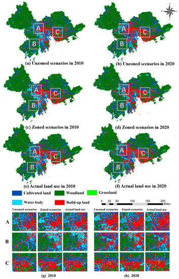
Figure 5.
Comparison of simulation results of land-use change in 2010 and 2020: (a) Simulation of unzoned scenarios in 2010; (b) Simulation of unzoned scenarios in 2020; (c) Simulation under zoned scenario in 2010; (d) Simulation under zoned scenario in 2020; (e) Actual data in the Pearl River Delta in 2010; and (f) Actual data in the Pearl River Delta in 2020. (g) Comparison of local area results in 2010; (h) Comparison of local area results in 2020.
The simulation results of the two scenarios are shown in Table 6, and the overall accuracy obtained in 2010 and 2020 under the zonal scenario is above 80%. The Kappa coefficient is above 0.8, which is much better than the results of the unzoned scenario simulation. From Table 7, it can be seen that the zoning scenario is much better than the unzoned scenario in the simulations of built-up land, cultivated land, and woodland. Specifically, in the simulation of built-up land in 2010, the error of the simulation results obtained from the zoning scenario is 0.70%, and the error of the results obtained from the unzoned simulation scenario is 40.92%; in the simulation of built-up land in 2020, the error of the simulation results obtained from the zoning scenario is 0.57%, and the error of the results obtained from the unzoned simulation scenario is 45.43%. In the simulation of cultivated land in 2010, the error of the simulation results obtained from the zoning scenario is 2.91%, and the error of the results obtained from the unzoned simulation scenario is 16.30%; in the simulation of cultivated land in 2020, the error of the simulation results obtained from the zoning scenario is 2.91%, and the error of the results obtained from the unzoned simulation scenario is 16.30%; in the simulation of cultivated land in 2020, the error of the simulation results obtained from the zoning scenario is 3.08%, and the error of the results obtained from the unzoned simulation scenario is 13.55%. Due to the more developed economy in Guangzhou and Shenzhen, the natural topography is relatively flat, and the topography is less undulating. Therefore, under the unzoned scenario, the accuracy of the simulation prediction results obtained by using factors such as DEM and slope as uniform natural factors influencing the PRD region are poor; under the zoning scenario, considering the drive of the relevant policies of the core cities of the PRD, the weights of economic and social factors driving factors are increased, and the weights of natural drivers are reduced in this study. This renders the simulation of the built-up land accurate. As woodlands are distributed mostly in suburban areas, their expansion is less influenced by roads. Therefore, the influence of roads on their conversion is reduced in the conversion rules of grassland expansion in Zhaoqing, Jiangmen, and Huizhou regions under the zoning scenario simulation. The simulation results of the woodland are closer to the real situation, and the accuracy is improved. For cropland expansion, the positive impacts include low elevation, low slope, distance from urban centers, and low population density. Correspondingly, the influence weights of these several influences are upgraded in the zoning scenarios, and transformation rules adapted to the changes of several factors are developed. This led to a significant improvement in accuracy. In summary, the simulated predictions of land-use change in the PRD region under the zoning scenario are better than those under the unzoned scenario.
Table 6.
Comparison of overall accuracies and Kappa coefficients for partitioned and unpartitioned scenarios.
Table 7.
Comparison between PHLUS and traditional model.
3.3. Land-Use Forecasting in the Pearl River Delta Based on PHLUS
According to the above zoning results, land-use projections for 2030 were carried out in each sub-zone, and the area and boundary of the region were used as the iterative termination conditions in each sub-zone. The projections for 2030 (Figure 6) show that the PRD region will maintain an increase in the area of built-up land and a decrease in the area of forest land and cultivated land, with this change being most pronounced in Zones 1 and 2. Compared with the land-use change in 2020, the proportion of built-up land in the PRD region increases from 14.69% to 19.95% in 2030 and is expected to reach 10,919 km2. The area of cultivated land and forest land will be reduced to 10,958 km2 and 26,880 km2, respectively, in 2030. The land-use change varies within different regions, but overall, it shows the conversion of cultivated and forested land to built-up land. The built-up land area in Sub-region 1 will reach 2727 km2 in 2030. This is the most obvious area for urban expansion, and built-up land will become the most dominant land type within the region in the future. This is influenced mainly by the policy and urban construction planning of the PRD region. Guangzhou and Shenzhen, as the core cities of sub-region one, are also the “twin cores” of the PRD. The national goal for their construction is to build them into a core development area with high-end functions and to reach the level of an international, modern metropolis. Cultivated land in Sub-area 2 is projected to be 1577 km2 in 2030, with little change compared with 2020. Forest land is forecast to decrease to 946 square kilometers in 2030, which is the main source of increase in built-up land. This is inseparable from the national policy of promoting the construction of coastal economic zone in recent years. The Zhuhai region has formed a new pattern of land and sea integration and linkage of port and industry. Sub-area III in the 2030 forecast shows that cultivated land, grassland, and built-up land all increase to varying degrees, and forest land shows a decreasing trend. Especially in the core urban areas, urban land is expanding more rapidly with the construction and development of economic development zones promoted by the state. The mainland types in Zones IV and V are cropland and forest land, which together account for more than 80% of the total area. This pattern is predicted to remain in 2030, but the area will decline. From the land-use change transfer Sankey diagram (Figure 7), we can see that the conversion out of cultivated land, forest land, and grassland is the largest. Cultivated land and forest land are transformed mainly into built-up land, and the converted areas are 2762 km2 and 1950 km2, respectively. Grassland is converted mainly into forest land and cropland, and the conversion out of built-up land is the smallest. From the results of the forecast, the PRD region will remain amid rapid development and construction in the future. The country and government need to weigh the relationship between the natural ecological environment and economic development in urban construction and economic development.
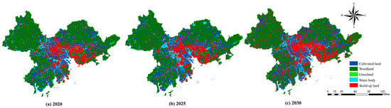
Figure 6.
Land-use change for Pearl River Delta from 2020 to 2030.
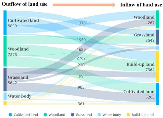
Figure 7.
Sankey map of land-use change transfer from 2020 to 2030.
4. Discussion
This study simulated land-use change in 2010 and 2020 on the basis of PHLUS and traditional CA-Markov model. The results show that the PHLUS significantly improves the simulation accuracy of land-use change. The model uses a partitioned approach to consider the effects of spatial heterogeneity on land-use change. In the current CA-Markov land-use change studies, the formation of suitability atlases for each land-use type is influenced by spatial variables. The driving factors selected are mostly natural and social factors, and the influence of economic factors on land-use change is usually ignored. However, economic and policy factors are often important drivers of urban development. There are important implications for changes in the spatial structure of land [52]. On the basis of existing studies, this study selected representative socio-economic factors that can reflect regional characteristics as driving factors, such as GDP and nighttime lighting data. The accuracy and realism of the simulation study of land-use change are improved. At present, partitioning the study area and developing different transition thresholds for conversion are the mainstream means to address this issue in the study of spatial heterogeneity of land-use change. The division of the study area and the determination of the conversion rules are conducive to the development of differentiated policies according to different regions in order to achieve a better simulation of land use change. In this process, regional characteristics of land-use change and regional policies need to be considered [53], although the method of double-constrained clustering takes into account the spatial location relationship between spatial objects and the attribute relationship between spatial objects in the partitioning. However, its partitioning results are usually divided only according to the principle of similarity, which lacks realistic and practical significance. The partition of future land development potential grades is based on the fuzzy hierarchical analysis method proposed in this study. The potential of natural, economic, and product development performance of land is considered comprehensively, and the development potential evaluation system is established by selecting natural conditions, ecological sensitivity, economic development, and spatial structure indicators [54,55]. The evaluation level zoning of future land development potential is obtained. This partitioning method can reflect the differences in potential land economic and ecological benefits among different regions.
However, the partitioning of the study area and the development of transfer rules remain challenges for PHLUS. Since partitioning is the prerequisite basis for developing transfer rules, its results are crucial to the accuracy of transfer rules for the entire study area [53]. Therefore, it plays an important role in the PHLUS simulation process. In this study, land development potential zoning methods were used for delineation, and the results showed that the combination of these algorithms was appropriate. However, there are some problems of unclear partitioning in the delineation results, and the selection of their indicators needs to be further studied and compared. This is to be improved in future studies. The method of improving the partitioning transition rules can obtain better performance. Analyzing the relationship between partitioning and transition rate and its influencing factors can help us to propose a more scientific method to calculate the transition rate of each cell, and the partitioning is derived from the scenario simulation.
5. Conclusions
In this study, PHLUS is used to integrate a CA model with a Markov model. A land development potential evaluation index system was established in the study on the basis of regional characteristics and development features. It can better evaluate the natural, economic, and productive performance for land-use change comprehensively and then highlight the spatial heterogeneity characteristics of land-use change with more quantitative results [56]. The driving factors chosen are mostly natural and social factors, while the influence of economic factors on land use change is often neglected. Combined with practical considerations, this paper argues that national/regional land conversion policies also have a driving role. This is because land regime changes profoundly affect the socio-economic development of land use. More precisely, land system and land economic development are a mutual influence process; land system change is about adapting to socio-economic development, and socio-economic development requires land system change and development [57]. This is why the impact of policies on the economy is translated in the study into the land potential assessment index of GDP. This paper divides the study area on the basis of the results of land development potential evaluation and explores the influencing factors that match the characteristics of regional land change. In the formulation of meta-cell conversion rules for land-use change simulation, this paper introduces global conversion probability and local conversion probability. Among them, the global conversion probability is determined by the MCE method by assigning weights to the spatial influence variables. The local transition probability is determined by the neighboring meta-cell states. Ultimately, the global transition probability and the local transition probability jointly determine the transition direction of the tuple. The model effectively solves the inaccuracy phenomenon of land growth simulation due to the spatial heterogeneity of regional development when the same factors affecting land expansion transformation are used to limit the land change simulation.
The PHLUS model introduced in this study is an expansion and improvement of the meta-automata model in the study of land-use change prediction. The model was applied to the Pearl River Delta urban agglomeration, and better simulation and prediction results were obtained. Compared with the traditional CA-Markov model, the PHLUS model proposed in this paper improves the overall accuracy of the simulation results by 11.55% and 7.14% in the 2010 and 2020 land-use simulations, respectively. Among them, the simulation effect for built-up land is the most significant, and the error between PHLUS simulation results and actual area in 2010 and 2020 is only 0.7% and 0.57%, respectively. Using PHLUS to forecast land-use change in the PRD region in 2030, we determined that the type of future land-use change in the PRD region is manifested mainly by the transfer from cultivated land and forest land to built-up land. Meanwhile, by 2030, the area of built-up land in the PRD region will reach 10,919 km2.
In particular, this study provides new theoretical support for the simulation of study areas with spatial heterogeneity or large differences in regional characteristics, such as urban clusters. In addition, the sub-regional land-use simulation and forecast is a new research model proposed compared with the traditional simulation according to the complete study area scope. The content of this study is beneficial to the government in formulating more reasonable and effective policies for fine-grained regional zoning management and coordinated regional development.
Author Contributions
Conceptualization, Q.W., D.L. and X.Z.; methodology, Q.W. and D.L.; validation, Q.W., D.L. and F.G.; data curation, Y.S.; writing—original draft preparation, Q.W.; writing—review and editing, Q.W., D.L. and F.G.; funding acquisition, D.L. All authors have read and agreed to the published version of the manuscript.
Funding
This research was supported by the Third Xinjiang Scientific Expedition of the Key Research and Development Program by Ministry of Science and Technology of the People´s Republic of China (No. 2022xjkk1104), the Fundamental Research Funds for the Central Universities (No. 2652019001), and the Open Fund of Key Laboratory of Urban Land Resources Monitoring and Simulation, Ministry of Natural Resources (No. KF-2020-05-063).
Data Availability Statement
Not applicable.
Acknowledgments
We thank Institute of Remote Sensing and Digital Earth, Chinese Academy of Sciences for providing the data used in this study.
Conflicts of Interest
The authors declare no conflict of interest.
References
- He, C.; Zhang, D.; Huang, Q.; Zhao, Y. Assessing the potential impacts of urban expansion on regional carbon storage by linking the LUSD-urban and InVEST models. Environ. Model. Softw. 2016, 75, 44–58. [Google Scholar] [CrossRef]
- Zhang, D.; Huang, Q.; He, C.; Wu, J. Impacts of urban expansion on ecosystem services in the Beijing-Tianjin-Hebei urban agglomeration, China: A scenario analysis based on the Shared Socioeconomic Pathways. Resour. Conserv. Recycl. 2017, 125, 115–130. [Google Scholar] [CrossRef]
- Song, W.; Pijanowski, B.C. The effects of China’s cultivated land balance program on potential land productivity at a national scale. Appl. Geogr. 2014, 46, 158–170. [Google Scholar] [CrossRef]
- Song, W.; Pijanowski, B.C.; Tayyebi, A. Urban expansion and its consumption of high-quality farmland in Beijing, China. Ecol. Indic. 2015, 54, 60–70. [Google Scholar] [CrossRef]
- Tobler, W.R. Cellular geography. Philos. Geogr. 1979, 20, 379–386. [Google Scholar] [CrossRef]
- Tong, X.; Feng, Y. A review of assessment methods for cellular automata models of land-use change and urban growth. Int. J. Geogr. Inf. Sci. 2020, 34, 866–898. [Google Scholar] [CrossRef]
- Guzman, L.A.; Escobar, F.; Peña, J.; Cardona, R. A cellular automata-based land-use model as an integrated spatial decision support system for urban planning in developing cities: The case of the Bogotá region. Land Use Policy 2020, 92, 104445. [Google Scholar] [CrossRef]
- Wu, H.; Li, Z.; Clarke, K.C.; Shi, W.; Fang, L.; Lin, A.; Zhou, J. Examining the sensitivity of spatial scale in cellular automata Markov chain simulation of land use change. Int. J. Geogr. Inf. Sci. 2019, 33, 1040–1061. [Google Scholar] [CrossRef]
- Bertoni, D.; Aletti, G.; Ferrandi, G.; Micheletti, A.; Cavicchioli, D.; Pretolani, R. Farmland use transitions after the CAP greening: A preliminary analysis using Markov chains approach. Land Use Policy 2018, 79, 789–800. [Google Scholar] [CrossRef]
- Wang, Y.F. Analysis of Land Use and Landscape Patterns in Fanyang Town Based on CA-Markov Model. Sichuan For. Explor. Des. 2015, 2, 4. [Google Scholar] [CrossRef]
- Iacono, M.; Levinson, D.; El-Geneidy, A.; Wasfi, R. A Markov chain model of land use change. TeMA J. Land Use Mobil. Environ. 2015, 8, 263–276. [Google Scholar] [CrossRef]
- Hamad, R.; Balzter, H.; Kolo, K. Predicting land use/land cover changes using a CA-Markov model under two different scenarios. Sustainability 2018, 10, 3421. [Google Scholar] [CrossRef]
- Karimi, H.; Jafarnezhad, J.; Khaledi, J.; Ahmadi, P. Monitoring and prediction of land use/land cover changes using CA-Markov model: A case study of Ravansar County in Iran. Arab. J. Geosci. 2018, 11, 592. [Google Scholar] [CrossRef]
- Mansour, S.; Al-Belushi, M.; Al-Awadhi, T. Monitoring land use and land cover changes in the mountainous cities of Oman using GIS and CA-Markov modelling techniques. Land Use Policy 2020, 91, 104414. [Google Scholar] [CrossRef]
- Fang, Z.; Song, S.; He, C.; Liu, Z.; Qi, T.; Zhang, J.; Li, J. Evaluating the impacts of future urban expansion on surface runoff in an alpine basin by coupling the LUSD-urban and SCS-CN models. Water 2020, 12, 3405. [Google Scholar] [CrossRef]
- Song, S.; Liu, Z.; He, C.; Lu, W. Evaluating the effects of urban expansion on natural habitat quality by coupling localized shared socioeconomic pathways and the land use scenario dynamics-urban model. Ecol. Indic. 2020, 112, 106071. [Google Scholar] [CrossRef]
- Liu, D.; Zheng, X.; Wang, H. Land-use Simulation and Decision-Support system (LandSDS): Seamlessly integrating system dynamics, agent-based model, and cellular automata. Ecol. Model. 2020, 417, 108924. [Google Scholar] [CrossRef]
- Ronneberger, K.; Berrittella, M.; Bosello, F.; Tol, R. Klum@Gtap: Spatially-Explicit, Biophysical Land Use in a Computable General Equilibrium Model; AgEcon Search: St. Paul, MN, USA.
- Mustafa, A.; Rienow, A.; Saadi, I.; Cools, M.; Teller, J. Comparing support vector machines with logistic regression for calibrating cellular automata land use change models. Eur. J. Remote Sens. 2018, 51, 391–401. [Google Scholar] [CrossRef]
- López, S. Modeling agricultural change through logistic regression and cellular automata: A case study on shifting cultivation. J. Geogr. Inf. Syst. 2014, 2014, 46914. [Google Scholar] [CrossRef]
- Xu, Q.; Wang, Q.; Liu, J.; Liang, H. Simulation of land-use changes using the partitioned ANN-CA model and considering the influence of land-use change frequency. ISPRS Int. J. Geo-Inf. 2021, 10, 346. [Google Scholar] [CrossRef]
- Islam, K.; Rahman, M.F.; Jashimuddin, M. Modeling land use change using cellular automata and artificial neural network: The case of Chunati Wildlife Sanctuary, Bangladesh. Ecol. Indic. 2018, 88, 439–453. [Google Scholar] [CrossRef]
- Hagenauer, J.; Helbich, M. Mining urban land-use patterns from volunteered geographic information by means of genetic algorithms and artificial neural networks. Int. J. Geogr. Inf. Sci. 2012, 26, 963–982. [Google Scholar] [CrossRef]
- Xu, T.; Gao, J.; Coco, G. Simulation of urban expansion via integrating artificial neural network with Markov chain–cellular automata. Int. J. Geogr. Inf. Sci. 2019, 33, 1960–1983. [Google Scholar] [CrossRef]
- Shafizadeh-Moghadam, H.; Helbich, M. Spatiotemporal variability of urban growth factors: A global and local perspective on the megacity of Mumbai. Int. J. Appl. Earth Obs. Geoinf. 2015, 35, 187–198. [Google Scholar] [CrossRef]
- Moghadam, H.S.; Helbich, M. Spatiotemporal urbanization processes in the megacity of Mumbai, India: A Markov chains-cellular automata urban growth model. Appl. Geogr. 2013, 40, 140–149. [Google Scholar] [CrossRef]
- Liu, D.; Zheng, X.; Zhang, C.; Wang, H. A new temporal–spatial dynamics method of simulating land-use change. Ecol. Model. 2017, 350, 1–10. [Google Scholar] [CrossRef]
- Lin, J.; He, P.; Yang, L.; He, X.; Lu, S.; Liu, D. Predicting future urban waterlogging-prone areas by coupling the maximum entropy and FLUS model. Sustain. Cities Soc. 2022, 80, 103812. [Google Scholar] [CrossRef]
- Liu, D.; Zheng, X.; Wang, H.; Zhang, C.; Li, J.; Lv, Y. Interoperable scenario simulation of land-use policy for Beijing–Tianjin–Hebei region, China. Land Use Policy 2018, 75, 155–165. [Google Scholar] [CrossRef]
- da Cunha, E.R.; Santos, C.A.G.; da Silva, R.M.; Bacani, V.M.; Pott, A. Future scenarios based on a CA-Markov land use and land cover simulation model for a tropical humid basin in the Cerrado/Atlantic forest ecotone of Brazil. Land Use Policy 2021, 101, 105141. [Google Scholar] [CrossRef]
- Liang, X.; Liu, X.; Li, D.; Zhao, H.; Chen, G. Urban growth simulation by incorporating planning policies into a CA-based future land-use simulation model. Int. J. Geogr. Inf. Sci. 2018, 32, 2294–2316. [Google Scholar] [CrossRef]
- Li, X.; Liu, Y.; Liu, X.; Chen, Y.; Ai, B. Knowledge transfer and adaptation for land-use simulation with a logistic cellular automaton. Int. J. Geogr. Inf. Sci. 2013, 27, 1829–1848. [Google Scholar] [CrossRef]
- Lin, J.; Li, X.; Wen, Y.; He, P. Modeling urban land-use changes using a landscape-driven patch-based cellular automaton (LP-CA). Cities 2023, 132, 103906. [Google Scholar] [CrossRef]
- Huang, Y.; Yang, B.; Wang, M.; Liu, B.; Yang, X. Analysis of the future land cover change in Beijing using CA–Markov chain model. Environ. Earth Sci. 2020, 79, 60. [Google Scholar] [CrossRef]
- Liu, J.; Liu, M.; Tian, H.; Zhuang, D.; Zhang, Z.; Zhang, W.; Tang, X.; Deng, X. Spatial and temporal patterns of China’s cropland during 1990–2000: An analysis based on Landsat TM data. Remote Sens. Environ. 2005, 98, 442–456. [Google Scholar] [CrossRef]
- Liu, J.; Kuang, W.; Zhang, Z.; Xu, X.; Qin, Y.; Ning, J.; Zhou, W.; Zhang, S.; Li, R.; Yan, C. Spatiotemporal characteristics, patterns, and causes of land-use changes in China since the late 1980s. J. Geogr. Sci. 2014, 24, 195–210. [Google Scholar] [CrossRef]
- Song, W.; Deng, X. Land-use/land-cover change and ecosystem service provision in China. Sci. Total Environ. 2017, 576, 705–719. [Google Scholar] [CrossRef] [PubMed]
- White, R.; Uljee, I.; Engelen, G. Integrated modelling of population, employment and land-use change with a multiple activity-based variable grid cellular automaton. Int. J. Geogr. Inf. Sci. 2012, 26, 1251–1280. [Google Scholar] [CrossRef]
- Allan, A.; Soltani, A.; Abdi, M.H.; Zarei, M. Driving Forces behind Land Use and Land Cover Change: A Systematic and Bibliometric Review. Land 2022, 11, 1222. [Google Scholar] [CrossRef]
- Wu, H.; Lin, A.; Xing, X.; Song, D.; Li, Y. Identifying core driving factors of urban land use change from global land cover products and POI data using the random forest method. Int. J. Appl. Earth Obs. Geoinf. 2021, 103, 102475. [Google Scholar] [CrossRef]
- Kasraian, D.; Raghav, S.; Miller, E.J. A multi-decade longitudinal analysis of transportation and land use co-evolution in the Greater Toronto-Hamilton Area. J. Transp. Geogr. 2020, 84, 102696. [Google Scholar] [CrossRef]
- Xie, H.; He, Y.; Xie, X. Exploring the factors influencing ecological land change for China’s Beijing–Tianjin–Hebei Region using big data. J. Clean. Prod. 2017, 142, 677–687. [Google Scholar] [CrossRef]
- Saputra, M.H.; Lee, H.S. Prediction of land use and land cover changes for north sumatra, indonesia, using an artificial-neural-network-based cellular automaton. Sustainability 2019, 11, 3024. [Google Scholar] [CrossRef]
- Gao, L.; Tao, F.; Liu, R.; Wang, Z.; Leng, H.; Zhou, T. Multi-scenario simulation and ecological risk analysis of land use based on the PLUS model: A case study of Nanjing. Sustain. Cities Soc. 2022, 85, 104055. [Google Scholar] [CrossRef]
- Wang, Q.; Guan, Q.; Lin, J.; Luo, H.; Tan, Z.; Ma, Y. Simulating land use/land cover change in an arid region with the coupling models. Ecol. Indic. 2021, 122, 107231. [Google Scholar] [CrossRef]
- Ke, X.; Deng, X.; Liu, C. Interregional Farmland Layout Optimization Model Based on the Partition Asynchronous Cellular Automata: A Case Study of the Wuhan City Circle. Prog. Geogr. 2010, 29, 1442–1450. [Google Scholar]
- Chen, Y.; Li, W.; Ren, L.; Li, J.; Ma, R. Changes in the Distribution of Rural Residential Land on a Coastal Plain. Resour. Sci. 2014, 36, 2273–2281. [Google Scholar]
- Wang, Y.; Ma, R.; Sun, D. Multi-dimensional Measurement of Land-island Metropolitan Area Structure. J. Ningbo Univ. (NSEE) 2015, 28, 63–68. [Google Scholar]
- Li, W.; Chen, Y.; Ma, R.; Yu, T.; Ren, L.; Li, J. Land-use pattern in coastal zone from the perspective of development potentiality: A case study of the southern bank of Hangzhou Bay. Geogr. Res. 2016, 35, 1061–1073. [Google Scholar]
- Yue, Q.; Liu, F.; Liu, Z. Comprehensive assessment of plain reservoir healthbased on fuzzy and hierarchy analyses. Hydro-Sci. Eng. 2016, 2, 62–68. [Google Scholar] [CrossRef]
- Xu, R.; Sun, J.; Han, H.; Zhou, L.; Yang, W. Simulation of Spatio-temporal Changes of Land Use Based on MCE-Markov-CA in Zhengzhou. Geogr. Geo-Inf. Sci. 2020, 36, 93–99. [Google Scholar]
- Wang, Q.; Wang, H. An integrated approach of logistic-MCE-CA-Markov to predict the land use structure and their micro-spatial characteristics analysis in Wuhan metropolitan area, Central China. Environ. Sci. Pollut. Res. 2022, 29, 30030–30053. [Google Scholar] [CrossRef] [PubMed]
- Ke, X.; Qi, L.; Zeng, C. A partitioned and asynchronous cellular automata model for urban growth simulation. Int. J. Geogr. Inf. Sci. 2016, 30, 637–659. [Google Scholar] [CrossRef]
- Dan, H.; Jing, Z.; Wei, G. An integrated CA-Markov model for dynamic simulation of land use change in Lake Dianchi Watershed. Acta Sci. Nat. Univ. Pekin. 2014, 50, 1095–1105. [Google Scholar] [CrossRef]
- Xiao, M.; Wu, J.; Chen, Q.; Jin, M.; Hao, X.; Zhang, Y. Dynamic change of land use in Changhua downstream watershed based on CA-Markov model. Trans. Chin. Soc. Agric. Eng. 2012, 28, 231–238. [Google Scholar] [CrossRef]
- Zhao, L.; Liu, X.; Liu, P.; Chen, G.; He, J. Urban expansion simulation and early warning based on geospatial partition and FLUS model. J. Geo-Inf. Sci 2020, 22, 517–530. [Google Scholar] [CrossRef]
- Dang, A.N.; Kawasaki, A. A review of methodological integration in land-use change models. Int. J. Agric. Environ. Inf. Syst. 2016, 7, 1–25. [Google Scholar] [CrossRef]


Disclaimer/Publisher’s Note: The statements, opinions and data contained in all publications are solely those of the individual author(s) and contributor(s) and not of MDPI and/or the editor(s). MDPI and/or the editor(s) disclaim responsibility for any injury to people or property resulting from any ideas, methods, instructions or products referred to in the content. |
© 2023 by the authors. Licensee MDPI, Basel, Switzerland. This article is an open access article distributed under the terms and conditions of the Creative Commons Attribution (CC BY) license (https://creativecommons.org/licenses/by/4.0/).