Abstract
Improving the water and land resource system efficiency can effectively alleviate the severe situation of water and land resources in China. Through the two-stage network DEA model, spatial autocorrelation analysis, multiple linear regression, and geographic weighted regression analysis, this paper revealed the change characteristics, distribution types, spatial correlation relationship, and main driving factors of China’s water and land resources system efficiency. The results show that the water and land resources system efficiency fluctuates widely in different regions. Water and land resources systems in nearly half of the provinces belong to the high development, low economic benefit transformation type, mainly distributed in southwestern and northwestern China. The economic benefit transformation is becoming the weak link of water and land resources system. The overall efficiency of water and land resource system has significant spatial positive correlation, and this correlation has an increasing trend. Low-Low Clusters occupy more provinces. The urbanization level, population density, proportion of output value of secondary and tertiary industries, and effective irrigation all have a positive impact on the overall efficiency of water and land resources system. The impact of the proportion of construction land is bidirectional and the per land pesticide application has negative impact in general.
1. Introduction
Water and land resources are fundamental natural resources and strategic economic resources, which can support production and life [1,2]. With the rapid growth of urbanization and industrialization, global water and land resources security is facing severe challenges [3,4]. As the most populous developing country in the world, China’s per capita water resources account for only one quarter of the world’s per capita level, and its per capita land area is less than one third of the world’s per capita level. Water and land resources are facing the problems of large absolute quantity but low per capita occupancy, serious waste, low utilization rate, uneven spatial distribution, and misalignment [5,6]. In recent years, the contradiction between the limited total amount of water and land resources, the problem of nonpoint source pollution of water and land resources, and the strong demand for water and land resources from economic growth have become more and more significant [7]. The total water consumption in China increased from 563.30 billion cubic meters in 2005 to 581.29 billion cubic meters in 2020, with an increase of 3.19%; and the agricultural and construction land area increased from about 688,969,000 hectares in 2005 to about 777,837,000 hectares in 2020, with an increase of 12.90%. The increased demand for water and land resources has caused a series of environmental problems such as groundwater overdraft, over-exploitation of sloping land, and soil erosion. Improving the water and land resource system efficiency is considered one of the current potential solutions [8]. Therefore, it is necessary to explore the actual situation of water and land resource system efficiency in China. Analyzing its characteristics and influencing factors will help ensure the balance of supply and demand of resource factors as well as promote high-quality development.
Water resources and land resources are closely linked, and the integrated study of water and land resources as an organic whole is becoming a research hotspot. In general, the research methods adopted mainly include water resources per unit area, Gini coefficient, Data Envelopment Analysis (DEA), etc. DEA is a method for measuring relative efficiency at different spatial scales, first proposed by Charnes, Cooper, and Rhodes in 1978 and has been widely used in resource efficiency evaluation. DEA can evaluate the relative efficiency of decision-making units (DMU) with multiple inputs and multiple outputs and does not require prior assumptions about the form of the production function, thus, its evaluation results are more objective and better reflect the utilization and matching of water and land resources [9,10].
Luan et al. [11] took the Sanjiang Plain as a study area, used DEA input oriented to evaluated agricultural land and water resources allocation efficient based on the water footprint. Xu et al. [12] analyzed the trend of agricultural water and land resources allocation efficiency in Gansu Province by using DEA model. Huang et al. [13] established a DEA model for water and land resources to analyze the matching degree of Sichuan Province. However, the DEA models used in these studies are mostly single-stage models, which treat water and land resources system as a “black box” with only inputs and outputs, ignoring the internal structure and inner operating mechanism of the system. Moreover, these studies hardly refine the process, and the premise is that the internal operation process of water and land resources system is absolutely effective by default. Obviously, this premise is too idealistic and does not conform to the actual operation of resource utilization and allocation. In contrast, the network DEA model considers the interactions between different stages and can integrate the efficiency evaluation of each network node in the system with the overall efficiency evaluation of the system. It is one of the methods applicable to the comprehensive assessment of the structural efficiency within a DMU [14]. In recent years, the network DEA model has been applied in several fields. Wu et al. [15] used the network DEA method to evaluate the overall efficiency, fund-raising efficiency, and fund-using efficiency of 27 Chinese commercial banks from 2006 to 2020 and put forward several policy implications based on the findings. Wang et al. [16] proposed a two-stage, network-based super DEA approach to investigate the overall efficiency and eco-efficiency of the sub-stages in China’s industrial system, including the production of three pollutant treatment stages. Liang et al. [17] developed an improved two-stage network DEA model under the assumption of variable returns to scale in terms of both weights and solution methods, then the overall efficiency of water resource systems, water use efficiency and wastewater treatment efficiency of 11 provinces in western China were measured.
In the construction of the network DEA model, the internal structure of the production unit should be fully considered. It is not only necessary to analyze the structural subordination between the internal sub-processes, but also to analyze whether there are shared inputs or shared outputs among the sub-processes, and whether there are intermediate inputs or intermediate outputs in addition to intermediate products in the sub-processes [18]. Although the complex production system with shared inputs among sub-processes are of important practical significance, few studies have been conducted on them. Chen et al. [19] took the lead in using the “arithmetic average” method to combine the sub-efficiency of two stages to measure the overall efficiency of the production system; Bi et al. [20] proposed to use the “geometric average” method to combine the sub-efficiency of two stages to measure the overall efficiency; Zha et al. [21] proposed the method of “multiplication aggregation” to combine the sub-efficiency of two stages to obtain the overall efficiency. However, the construction of these models seems to undermine the objective principle of performance evaluation. The reason is that the weight combination relationship between the sub-process efficiency is usually not directly available to decision makers, and the uniform aggregation of pre-defined sub-efficiency does not take into account the differences among production systems. From the perspective of system, it is necessary to improve the efficiency measurement model of the associated production system with shared inputs. We tried to construct a two-stage network DEA efficiency measurement and decomposition model with shared inputs, which not only fully considers the production information of intermediate products and the dynamic allocation information of input factors, but also eliminates the need to establish the way and weight of sub-efficiency aggregation into system efficiency in advance and apply it to the measurement of water and land resources system efficiency. To the best of our knowledge, limited work has been done in terms of implementing network DEA model with shared inputs to the water and land resources system efficiency. Further, there is a lack of comprehensive evaluation for the efficiency of the internal structure in the system. Establishing applicable model and evaluation method for measuring the water and land resources system efficiency is worthwhile.
Therefore, based on a macroeconomic level and the characteristics of water and land resource utilization, we divided the water and land resources system into two sub-stages: water and land resources development stage and economic benefit transformation stage. Since the sub-stage processes are recursively related, a series structured network DEA model was constructed. This model can simultaneously measure the overall efficiency, development efficiency and economic benefit transformation efficiency of water and land resources system. In the study, the water and land resources system efficiency from 2005 to 2020 was elaborated, the measured values of efficiency at different stages were used as a basis to classify and evaluate water and land resources system in different regions according to their characteristics, and the aggregation characteristics of water and land resources system efficiency were analyzed by using spatial autocorrelation. In addition, relevant indicators were selected from social, economic, and ecological levels, and the GWR model was used to reveal the influencing factors of water and land resources system efficiency and explore the path to improve the water and land resources system efficiency. This study provided a reference basis for achieving optimal regional allocation and promoting sustainable utilization and management of resources. The other parts of the paper are organized as follows: Section 2 contains the scope of the study, research methodology, and data sources; Section 3 gives the results and analysis; Section 4 contains the conclusions and discussion.
2. Data and Methodology
2.1. Study Area
The study area includes 31 provinces, municipal cities, and autonomous regions of mainland China. Due to limitations in available data, Hong Kong, Macao, and Taiwan were not considered in our study. Considering the imbalance of economic development and spatial distribution of resources, there is a significant regional difference in terms of water and land resources usage pattern. For example, the distribution of water resources in South China is much more abundant than that in northern China. Thus, China was divided into six areas based on physical geography and socio-economic conditions: the Northeast Region (NER), Central South Region (CSR), East Region (ER), North Region (NR), Northwest Region (NWR), and the Southwest Region (SWR) in Figure 1.
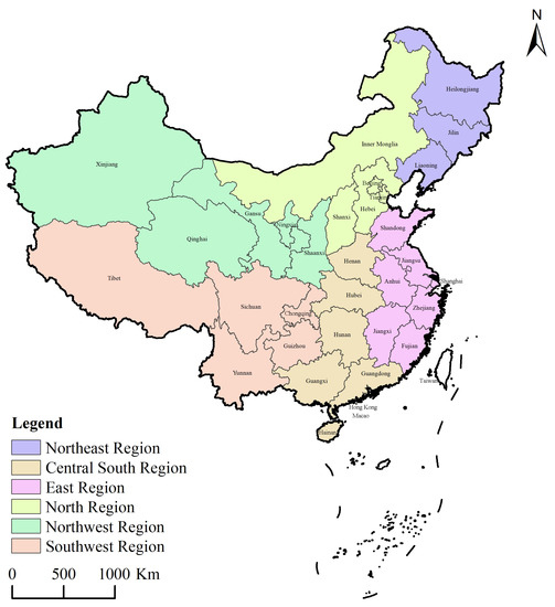
Figure 1.
Study area.
2.2. Two-Stage Network DEA Model with Shared Input Correlations
Since the use of land and water resources is a complex and mutually influencing process, the internal structure of the system cannot be ignored. The water and land resources system at the macro level is linked by several sub-stages with different functions, each sub-stage uses its own input to complete the corresponding output, together forming a large system to complete the overall resource use and output activities. We divided the water and land resources system into two sub-stages: development and economic benefit transformation [17,22,23]. In the first sub-stage, water and land resources (total water resources and land area), human resources (labor force), and material resources (fixed asset investment), which represent the initial cost inputs, are used as input indicators, water consumption and agricultural and construction land area, which reflect the development situation, are used as output indicators. The second sub-stage is a continuation of the first sub-stage, since human and material resources are always used in both sub-stages, they are regarded as shared inputs of both stages. Water consumption and agricultural and construction land area produced in the first stage are regarded as intermediate products and are also used as inputs in the second stage. The total production is considered as the output of the second stage. A two-stage network DEA model with shared input correlations is constructed, and its structure is shown in Figure 2.
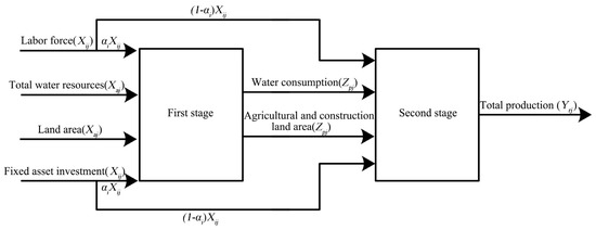
Figure 2.
The structure of two-stage network DEA model for water and land resources systems with shared input correlations.
Based on this structure, under the assumption of constant returns to scale (CRS), the input was minimized with at least the existing level of output (input oriented), we decomposed the system efficiency after calculating it based on a comprehensive consideration of the production information of each sub-system, and constructed a convex linear combination relationship between system efficiency and sub-efficiency in the context of the optimal relative practical efficiency of the system [24,25,26]. It is assumed that in , , act as shared inputs in the first and second stages, respectively. The parameters and denote the weight structures of shared inputs in different stages, respectively. The weights of independent inputs in the first stage are denoted by parameters . In addition, play dual roles as both first-stage outputs and second-stage inputs, the parameters and denote the weight structures of as first-stage outputs and second-stage inputs, respectively. The weight of is represented through the parameter . Therefore, the combined input of the first process is and the combined output is ; the combined input of the second process is and the combined output is . In the specific efficiency calculation, for , are set with reference to the treatment of Wang et al. [27], weakness of shared inputs at any stage cannot promote the overall efficiency of the water and land resources system, so their distribution proportion should not have a large deviation. Considering the combined inputs and outputs of the two sub-stages together, the overall efficiency of must satisfy not only the whole constraint but also the local constraint that constrains the two sub-stage processes independently, and the calculation formula is as follows:
Let , with the help of the Charnes-Cooper transformation [28], the fractional programming can be reduced to mathematical programming solution as follows:
In Equation (2), , , , , , . In order to prevent the optimal values of , , , , and from being 0 when finding the optimal solution, their lower bounds are set to ε, i.e., non-Archimedean infinitesimal. The value of ε is limited by the overall scale of inputs or outputs, rather than being set arbitrarily. Since Equation (2) is still a nonlinear programming, it can be simplified by making , for the convenience of solution. The nonlinear programming can be transformed into a directly solved equivalent linear programming as follows:
Linear programming describes the overall efficiency of the , with the help of Equation (3), the optimal combined solution of , , , , , , and can be obtained, and the efficiency values of the two sub-stages can be further calculated as follows:
2.3. Spatial Autocorrelation Analysis
Spatial autocorrelation analysis reflects the degree of spatial dependence among variables within a geographic area. The two main types of spatial autocorrelation analyses that can be conducted are global analyses and local analyses. Global Moran’s I can be used to determine the degree of spatial clustering or dispersion of variables for the entire study area [29]. The calculation formula is as follows:
where wij is the matrix of the spatial weight; n is the number of samples; xi and xj are the values of variable x at the location i and j, respectively; is the average value of variable x. Moran’s I > 0 indicates positive spatial correlation, and larger values correspond to stronger spatial correlation. Conversely, Moran’s I < 0 indicates negative spatial correlation. If Moran’s I equals 0, the spatial distribution of the variable is random.
Local autocorrelation analysis (LISA) can be employed to calculate the Local Moran’s I of all provincial administrative regions, the calculation formula is as follows:
Spatial associations are commonly divided into four categories: high–high cluster, low–low cluster, low–high outlier, and high–low outlier [30]. The first two categories indicate that the level (high or low) of the variable in this province is consistent with adjacent provinces, whereas the last two categories indicate that the level (high or low) of the variable in this province is different from adjacent provinces.
2.4. Geographically Weighted Regression (GWR) Analysis
To further explore the influencing factors of water and land resources system efficiency, we selected population density, urbanization level, proportion of output value of secondary and tertiary industries, effective irrigation rate, proportion of construction land, and per land pesticide application as independent variables and annual overall efficiency values of water and land resources system in 31 provincial administrative regions as dependent variables to establish regression model [31,32,33,34]. After selecting the potential drivers, we performed collinearity diagnosis based on the ordinary least squares (OLS) regression model and eliminated potential drivers with a variance inflation factor (VIF) greater than 7.5. OLS regression is a global statistical method that estimates the relationship between independent variables and a dependent variable. With the input of the explanatory variables and the efficiency indices, OLS can output the coefficients that indicate the direction and magnitude of the impact from the independent variables. Nevertheless, due to non-stationary or heterogeneous characteristics of most spatial patterns, a widely applied local regression model, GWR, has been applied in many applications to capture spatially varied relationships between multiple variables [35]. Compared to the global regression models such as OLS, GWR models the local relationships between predictors and a dependent variable as follows:
where yi and xij are the dependent and independent variables, respectively; β0 and βj present the intercept and regression coefficient, respectively; ui, vi is the coordinate that represents the location of observation i; k is the number of independent variables; and εi represents error. The adjusted coefficient of determination (Adj.R2) and corrected Akaike information criterion (AICc) serve as a measure of goodness of fit to determine whether a global or local model should be applied to have a better interpretation for the patterns in the analyzed data [36].
2.5. Data Sources
Socio-economic indicators such as labor force, fixed asset investment, and total production were obtained from China Statistical Yearbooks and Local Statistical Yearbooks. Total water resources and water consumption were obtained from Water Resource Bulletins. Land area and agricultural and construction land area were obtained from China Land and Resources Statistical Yearbook. Additionally, the interpolation method was used to supplement some missing data.
3. Results and Analysis
3.1. Measurement of Water and Land Resources System Efficiency
The overall efficiency and sub-stages efficiency of water and land resources system in 31 provincial administrative regions from 2005 to 2020 were measured, and the results are calculated in Table 1 (due to the length, only the results in 2005, 2010, 2015, and 2020 are shown). The overall efficiency of water and land resource system fluctuates widely in different regions. Beijing, Tianjin, Liaoning, and Chongqing show an upward trend. Among them, Liaoning shows the most obvious rise, with a change rate of 0.0144/a, mainly due to the local area giving full play to its resource advantages, strengthening the economical use of resources, promoting industrial integration and the construction of a modern production system, and encouraging high-quality development. Hebei, Shanxi, Inner Mongolia, Jilin, Heilongjiang, Jiangsu, Zhejiang, Anhui, Fujian, Jiangxi, Shandong, Henan, Hubei, Hunan, Guangdong, Guangxi, Hainan, Sichuan, Guizhou, Yunnan, Tibet, Shaanxi, Gansu, Qinghai, Ningxia, and Xinjiang show a downward trend. Among them, Guangdong shows the most obvious decline, with a change rate of −0.0315/a, mainly due to the decreasing cultivated land, serious soil erosion, and shrinking resource potential. Shanghai remains unchanged and the overall efficiency has been relatively efficient.

Table 1.
Water and land resources system efficiency of 31 provincial administrative regions in China.
In the first stage efficiency of water and land resources system in each region, Beijing, Tianjin, Hebei, Shanxi, Liaoning, Jilin, Heilongjiang, Jiangsu, Zhejiang, Jiangxi, Shandong, Henan, Hubei, Hunan, Hainan, Chongqing, Sichuan, Guizhou, Yunnan, and Shaanxi show an upward trend with a rate of change between 0.0005/a–0.0327/a, while Anhui, Fujian, Guangdong, Guangxi, and Gansu show a downward trend with a rate of change between −0.0156/a–−0.0009/a, Inner Mongolia, Shanghai, Tibet, Qinghai, Ningxia, and Xinjiang remain unchanged, are in relatively effective development efficiency. In the second stage of the efficiency of water and land resources system in each region, Liaoning shows an upward trend with a change rate of 0.0164/a, while Tianjin, Hebei, Shanxi, Inner Mongolia, Jilin, Heilongjiang, Jiangsu, Zhejiang, Anhui, Fujian, Jiangxi, Shandong, Henan, Hubei, Hunan, Guangdong, Guangxi, Hainan, Chongqing, Sichuan, Guizhou, Yunnan, Tibet, Shaanxi, Gansu, Qinghai, Ningxia, and Xinjiang show a downward trend with a rate of change between −0.0526/a–0.0038/a, Beijing and Shanghai remain unchanged, are in relatively effective of economic benefit transformation efficiency.
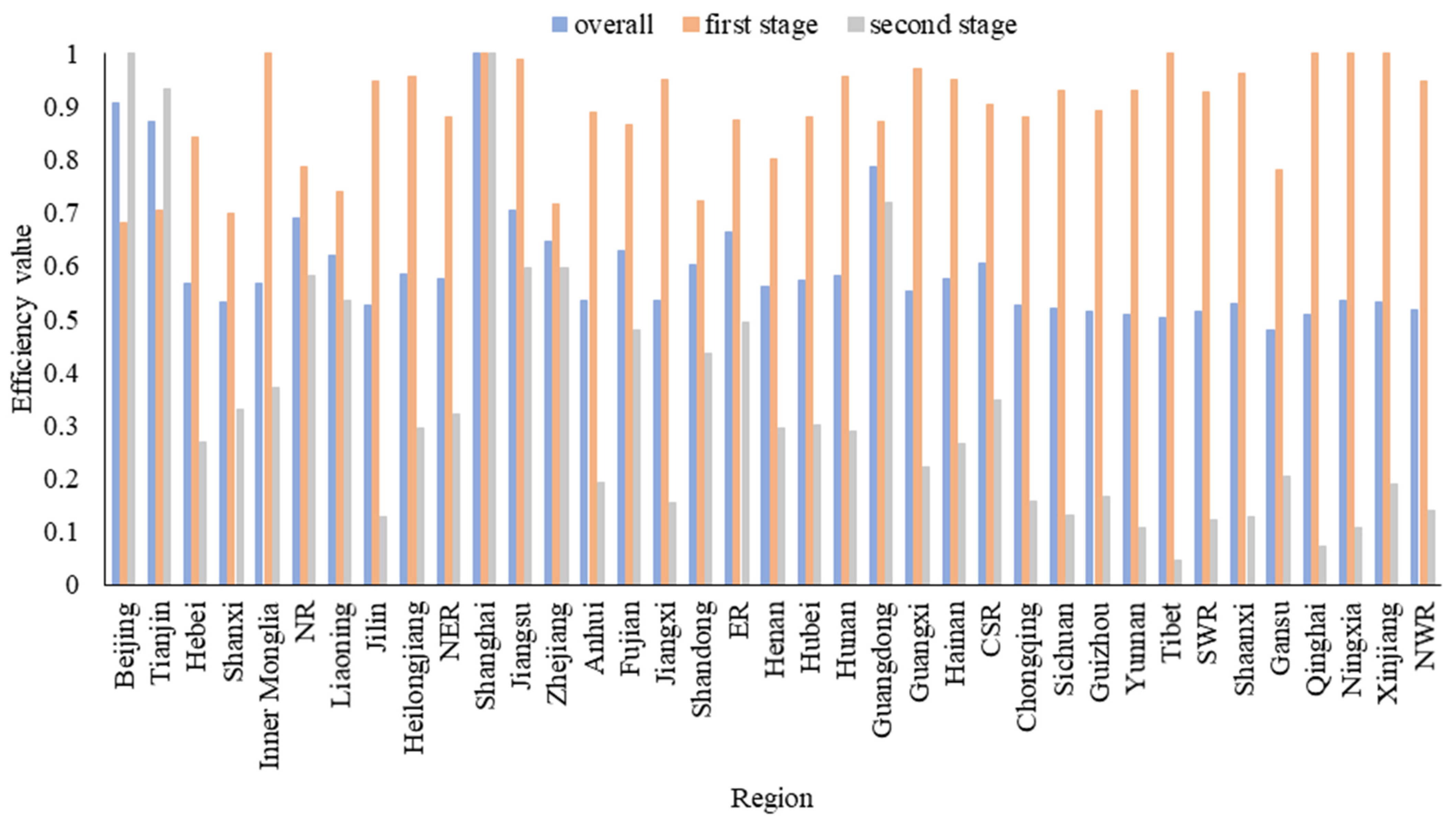
Based on the results of overall efficiency and sub-stage efficiency of water and land resources system in 31 provincial administrative regions of China from 2005 to 2020, the relationship between overall efficiency and sub-stage efficiency in different regions was analyzed, as shown in Figure 3. The average efficiency values of Tianjin, Hebei, Shanxi, Inner Mongolia, Liaoning, Jilin, Heilongjiang, Jiangsu, Zhejiang, Anhui, Fujian, Jiangxi, Shandong, Henan, Hubei, Hunan, Guangdong, Guangxi, Hainan, Chongqing, Sichuan, Guizhou, Yunnan, Tibet, Shaanxi, Gansu, Qinghai, Ningxia, and Xinjiang in the first stage are higher than the average efficiency values in the second stage. The average efficiency values of Beijing and Tianjin in the second stage are higher than the average efficiency values in the first stage. The average efficiency values in the first and second stages of Shanghai are 1. The average efficiency values of most regions in the first stage are higher than the average efficiency values in the second stage, indicating that economic benefit transformation is the weak link of the water and land resources system in most regions of China. The overall average efficiency, the first-stage average efficiency and the second-stage average efficiency have obvious regional differences, all showing high in the Eastern coastal areas, including Shanghai and Tianjin, and low in the Western inland areas, including Gansu and Qinghai.

Figure 3.
Average value of water and land resources system efficiency in 31 provincial administrative regions from 2005 to 2020.
3.2. Characteristics of Water and Land Resources System Efficiency in Different Regions
According to the average value of the development efficiency (0.887) and the average value of the economic benefit transformation efficiency (0.346) of China’s water and land resources system from 2005 to 2020, the water and land resources system of different provincial administrative regions were classified by characteristics into low development—low economic benefit transformation (Low—Low type), low development—high economic benefit transformation (Low—High type), high development—low economic benefit transformation (High—Low type), and high development—high economic benefit transformation (High—High type). The specific classification is shown in Figure 4.
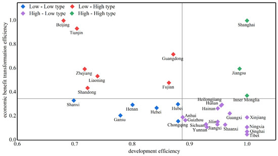
Figure 4.
Two-dimensional distribution map of development efficiency and economic benefit transformation efficiency of water and land resources system.
Hebei, Shanxi, Henan, Hubei, Chongqing, and Gansu belong to the Low—Low type, accounting for about 19.4% of the total number of provinces, mainly in Northern China, where water and land resources are used haphazardly and struggle to achieve development with benefits. They need to fully understand their own resource characteristics, strengthen the construction of resource allocation projects, guide the orderly use of effective water sources and available land, and pay attention to investment to fundamentally reverse the situation of weak development and economic benefit transformation of water and land resources.
Beijing, Tianjin, Liaoning, Zhejiang, Fujian, Shandong, and Guangdong belong to the Low—High type, accounting for about 22.6% of the total number of provinces, mainly located in the Huang-Huai-Hai Plain and the Middle-Lower Yangtze Plain in China, where water resources are relatively abundant and land resources are relatively scarce. The imbalanced distribution of water and land resources has prevented them from large-scale development and utilization. However, their superior location conditions makes them have the advantage of economic benefits transformation. They need to improve the sustainable utilization capacity of water and land resources, and strengthen the support and guarantee capacity of water and land resources for economic and social development.
Jilin, Heilongjiang, Anhui, Jiangxi, Hunan, Guangxi, Hainan, Sichuan, Guizhou, Yunnan, Tibet, Shaanxi, Qinghai, Ningxia, and Xinjiang belong to the High—Low type, accounting for about 48.3% of the total number of provinces, mainly in southwest and northwest China, where water and land resources are relatively abundant and highly developed, but the beneficial conversion of late construction to early resource development has been neglected. On the basis of maintaining the current advantages in the development and utilization of water and land resources, they should shift their focus on the stage of economic benefits transformation, establish and improve the management and use mechanism of water and land resources, actively implement the financial and industrial policies related to water and land resources, and closely integrate with market demand to realize the value of water and soil resources.
Inner Mongolia, Shanghai, and Jiangsu belong to the High—High type, accounting for about 9.7% of the total number of provinces, mainly in Eastern China, where development and economic transformation have driven the utilization of water and land resources in the surrounding areas and achieve good results. They need to strengthen the protection and management of environment on the basis of maintaining the current advantages of development and economic transformation of water and land resources system, avoid damage to ecological environment in the process of resource development and economic transformation, formulate water quota and land red line, establish a perfect system of water and land resources guarantee, and achieve the strategic objectives of conservation, protection, allocation and sustainable use of water and land resources.
3.3. Spatial Correlations of Water and Land Resources System Efficiency in China
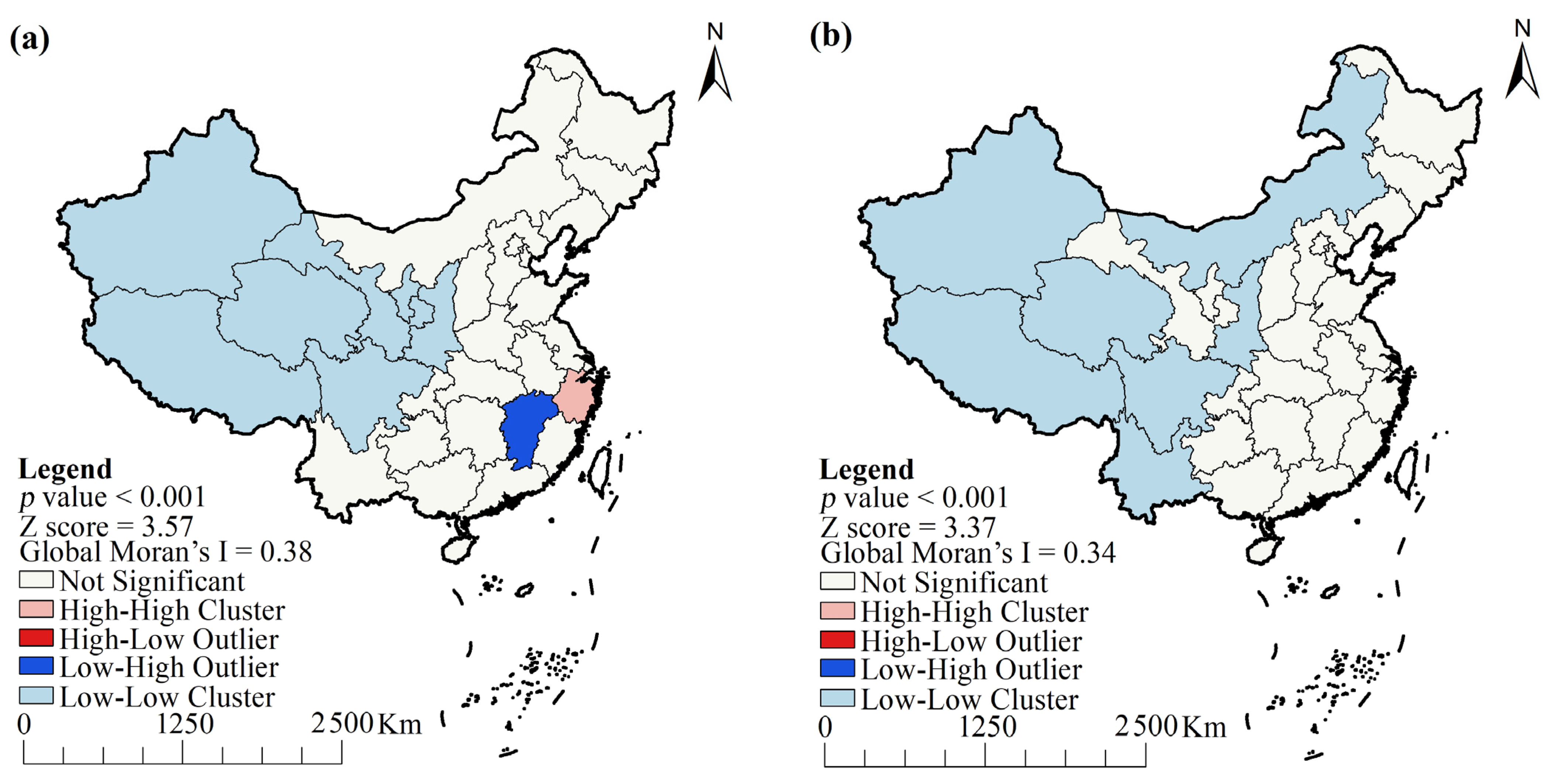
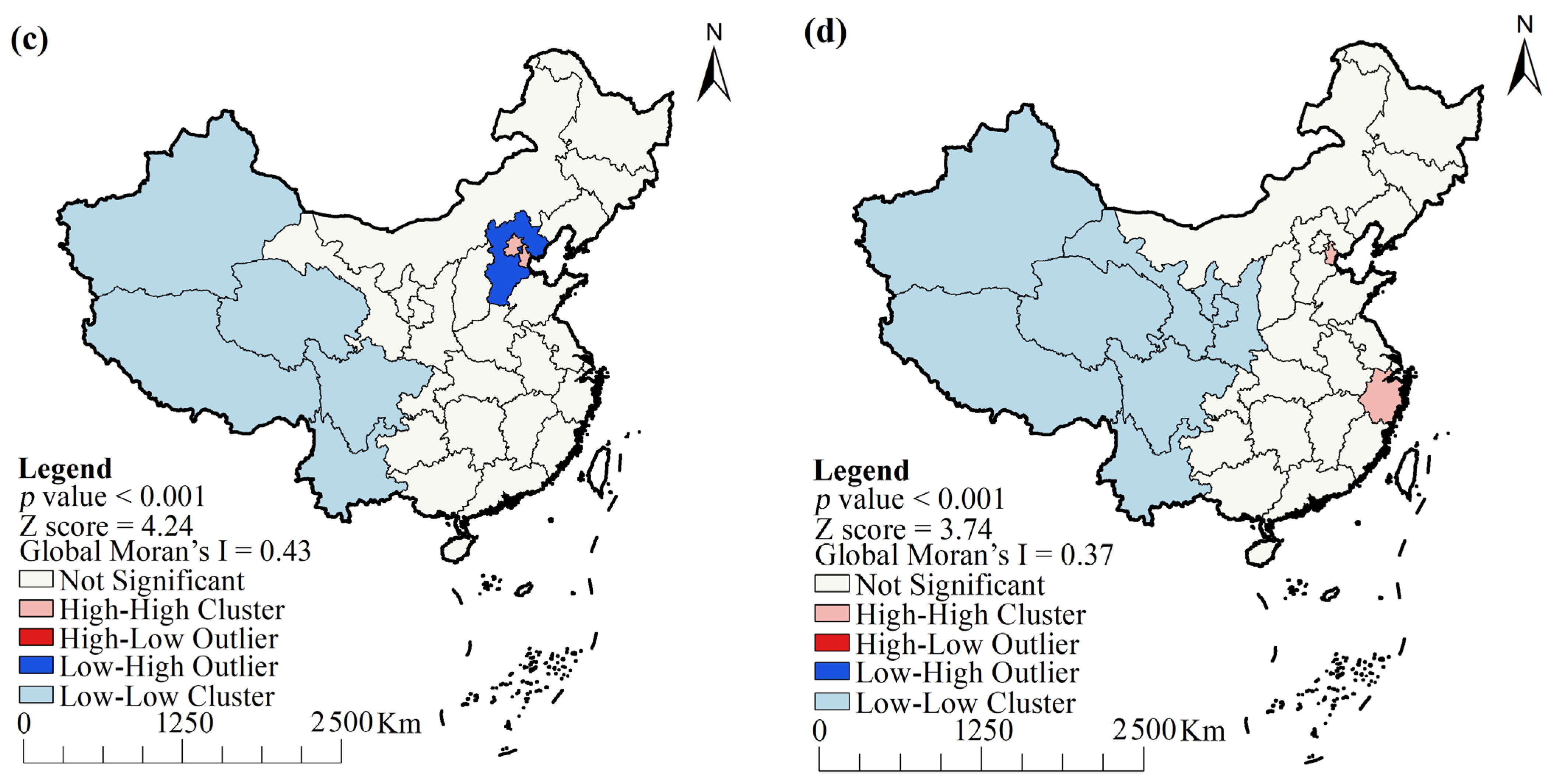
In order to clarify the spatial correlation characteristics of water and land resources system efficiency, the overall efficiency of China’s water and land resources system from 2005 to 2020 was tested by using global autocorrelation and local autocorrelation. The spatial autocorrelation patterns of water and land resources system efficiency in 2005, 2010, 2015 and 2020 are shown in Figure 5. From 2005 to 2020, the Global Moran’s I indices of the overall efficiency of water and land resources system in China are all above 0.30, with p-values less than 0.001, indicating that the overall efficiency of the water and land resource system has significant spatial positive correlation and aggregation at the 0.001 level. Among them, the Global Moran’s I index in 2020 is the highest, at 0.43. The spatial positive correlation has an increasing trend.
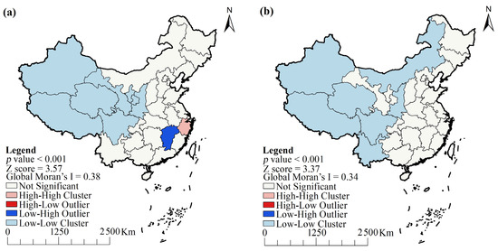
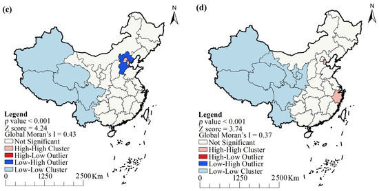
Figure 5.
Spatial autocorrelation of overall efficiency of water and land resources system in 2005 (a), 2010 (b), 2015 (c), and 2020 (d).
In 2005, the spatial autocorrelation of the overall efficiency of water and land resources system in Zhejiang presents a distribution pattern of High-High Cluster, Low-High Outlier is concentrated in Jiangxi, Low-Low Clusters are concentrated in Xinjiang, Tibet, Qinghai, Gansu, Ningxia, Shaanxi, and Sichuan, and there are no High-Low Outlier areas. In 2010, Low-Low Clusters are concentrated in Xinjiang, Tibet, Qinghai, Inner Mongolia, Shaanxi, Sichuan and Yunnan, there are no High-High Cluster areas, High-Low Outlier areas, or Low-High Outlier areas. In 2015, High-High Clusters are concentrated in Beijing and Tianjin, Low-High Outlier is concentrated in Hebei, Low-Low Clusters are concentrated in Xinjiang, Tibet, Qinghai, Sichuan and Yunnan, and there are no High-Low Outlier areas. In 2020, High-High Clusters are concentrated in Tianjin and Zhejiang, Low-Low Clusters are concentrated in Xinjiang, Tibet, Qinghai, Gansu, Ningxia, Shaanxi, Sichuan, and Yunnan, there are no High-Low Outlier areas and Low-High Outlier areas. On the whole, High-High Clusters are mainly concentrated in the North China Plain and Southeast Coast. Low-Low Clusters occupy more provinces, mainly in western and northern China, this distribution pattern has a tendency to migrate to the southwest in recent years. Isolated high or low value areas are difficult to emerge.
3.4. Influencing Factors of Water and Land Resources System Efficiency
Previous papers had shown that there was a spatial correlation in the overall efficiency of China’s water and land resources system. Therefore, the GWR model can be further used to analyze the spatial differences of the influencing factors on overall efficiency of China’s water and land resources system. In order to illustrate the applicability of GWR, we used the OLS and GWR models to simulate as shown in Table 2. The R2 and Adjusted R2 of the GWR model are larger than those of the OLS model, indicating that the simulation effect is more accurate and representative. Meanwhile, the AICc of the GWR model is smaller than that of the OLS model, and the difference is greater than 3.0, which demonstrated that the GWR model is more applicable [36]. Therefore, the GWR model can accurately explain the relationship between average overall efficiency of water and land resources system from 2005 to 2020 and each explanatory variable and the spatial heterogeneity.
Table 2.
The performance of the OLS and GWR models.
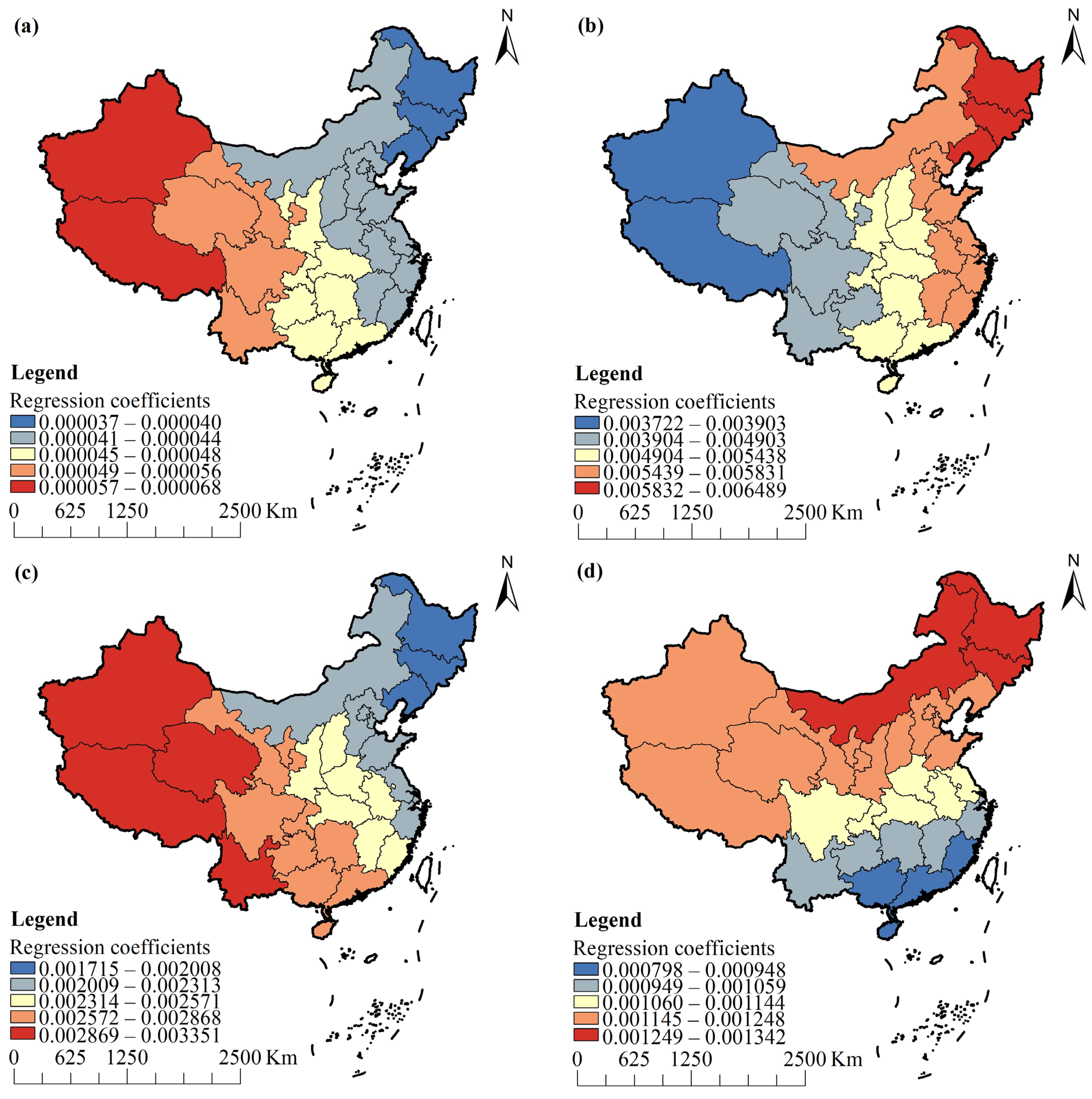
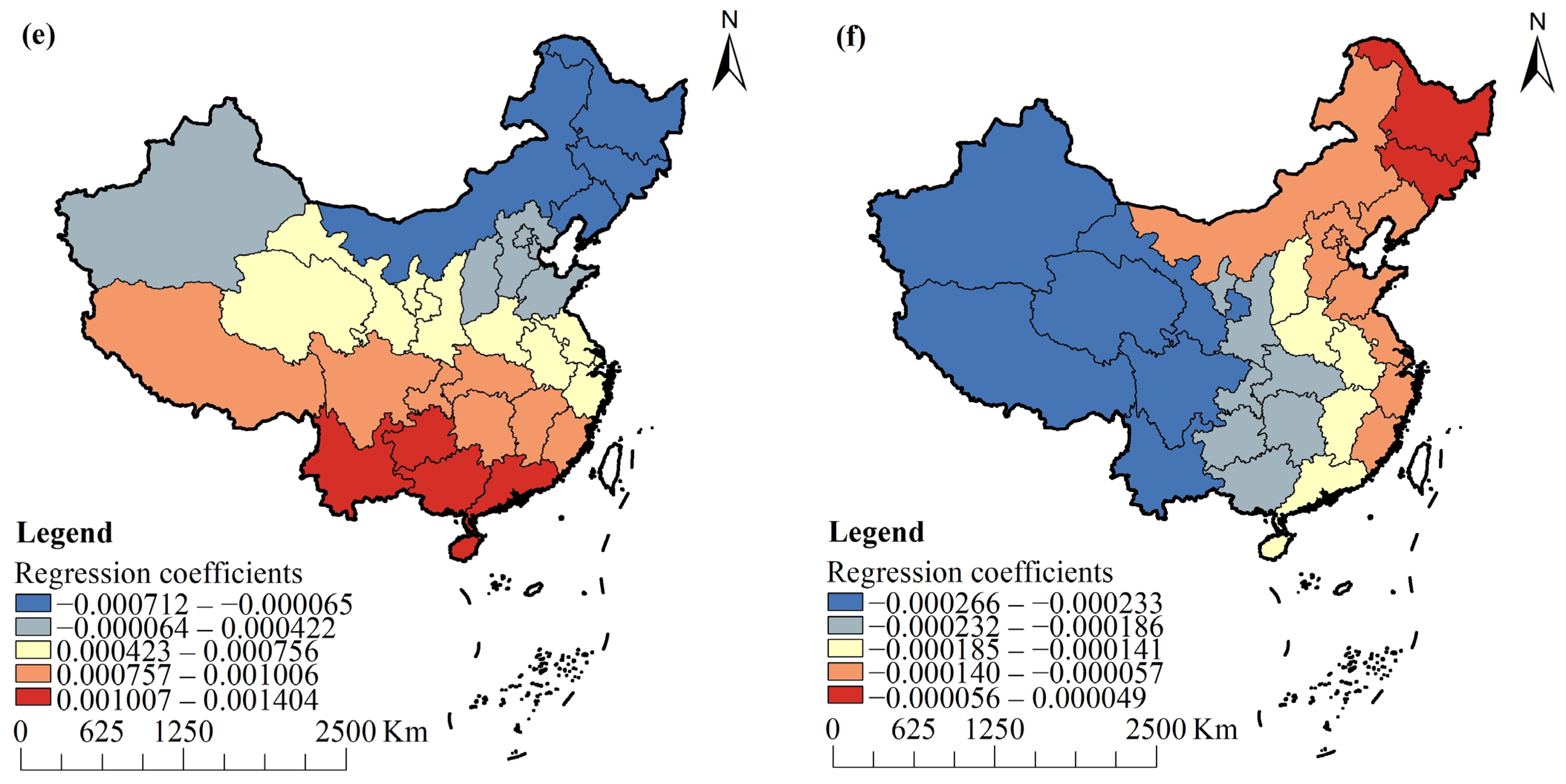
The spatial distribution of GWR model regression coefficients of population density, urbanization level, proportion of output value of secondary and tertiary industries, effective irrigation rate, proportion of construction land and per land pesticide application are shown in Figure 6. Population density, urbanization level, the proportion of output value of secondary and tertiary industries, and effective irrigation rates all have positive effects on the efficiency of water and land resources system in all provinces in China, of which urbanization level is the most significant, and the overall spatial pattern decreases from northeast to southwest. The spatial pattern of population density and the proportion of output value of secondary and tertiary industries is similar, with high values in the Western Region and low values in the Northeastern Region. The intensity of human activities and the level of economic development in the Western Region are low, so the increase in population density and the proportion of output value of secondary and tertiary industries has a positive impact on the efficiency of water and land resources system [37]. Northeastern China is rich in natural resources and has great potential for agricultural development, the promotion of population density and proportion of secondary and tertiary industries on the efficiency of water and land resources system is relatively weak [38]. The spatial pattern of effective irrigation rate decreases from north to south, which is mainly due to the difference in topography and modern production level [39]. The Northern Region has mostly vast plains, where large-area water conservancy irrigation and mechanical seeding can promote the full utilization of water and land resources. In contrast, the Southern Region has dense river networks, finely fragmented land distribution, and relatively developed modern irrigation technology. The effect of proportion of construction land on water and land resources system efficiency in China’s provinces is bidirectional, both promoting and inhibiting (positive or negative regression coefficients). Heilongjiang, Jilin, Liaoning, and Inner Mongolia have a negative relationship between the proportion of construction land and the efficiency of water and land resources system, where the non-agricultural land phenomenon possible brought about by the increase of the proportion of construction land share will cause a decrease in the efficiency of water and land resources system [40]. The remaining provinces have a positive relationship, where the increase in the proportion of construction land will bring economic transformation benefits to water and land resource systems [41]. The per land pesticide application has a negative correlation with the efficiency of water and land resources system on the whole, the positive correlation only in Heilongjiang. This indicates that the increase in per land pesticide application will inevitably cause some damage to the ecological environment, thus causing pressure on the water and land resources system [42,43].

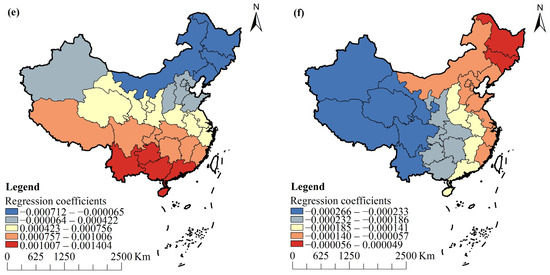
Figure 6.
Distribution of the regression coefficient of overall efficiency of water and land resources system with population density (a), urbanization level (b), proportion of output value of secondary and tertiary industries (c), effective irrigation rate (d), proportion of construction land (e), and per land pesticide application (f).
4. Conclusions and Discussion
4.1. Conclusions
The two-stage network DEA model with shared inputs was used to measure the overall efficiency, development efficiency, and economic benefit transformation efficiency of water and land resources system in 31 provincial administrative regions of China in this paper. We constructed a network DEA efficiency measurement and decomposition model for a two-stage production system with shared inputs among internally related sub-processes based on the standard DEA ratio approach. This model construction method is more in line with the objective evaluation principle of DEA, and does not need to use “arithmetic average”, “geometric average”, and “multiplicative aggregation” to set the two-stage efficiency subjectively [19,20,21]. From the overall perspective of each sub-process, the transformation information of intermediate products and input resource allocation information are fully considered. The construction idea of this model is general, which can be easily extended and constructed into a production system efficiency measurement model with more complex internal transformation structure [26,44,45]. On the basis, the classification characteristics, spatial correlation relationship and influencing factors of water and land resources system efficiency in different regions were analyzed through spatial autocorrelation analysis, multiple linear regression and geographic weighted regression analysis. The following conclusions are drawn:
- (1)
- The overall efficiency of water and land resource system fluctuates widely in different regions, with a rate of change between −0.0315/a–0.01448/a. The average efficiency values of most provinces in the first stage are higher than the average efficiency values in the second stage, indicating that economic benefit transformation is the weak link of the water and land resources system. The overall average efficiency, the first-stage average efficiency and the second-stage average efficiency of the water and land resource system, shows obvious regional differences, all showing them to be high in the eastern coastal areas, and low in the western inland areas.
- (2)
- The low development-low economic benefit transformation type of water and land resources system is mainly distributed in northern China, the low development-high economic benefit transformation type is mainly distributed in the Huang-Huai-Hai Plain and the Middle-Lower Yangtze Plain China, the high development-low economic benefit transformation type is mainly distributed in southwestern and northwestern China, and the high development-high economic benefit transformation type is mainly distributed in eastern China.
- (3)
- The overall efficiency of the water and land resource system has significant spatial positive correlation, and this spatial positive correlation has an increasing trend. High-High Clusters are mainly concentrated in the North China Plain and Southeast Coast. Low-Low Clusters occupy more provinces, mainly in western and northern China.
- (4)
- The influence of each driving factor on the overall efficiency of water and land resources system has spatial heterogeneity. The urbanization level has the most significant positive impact, with spatial pattern decreasing from northeast to southwest. Population density, the proportion of output value of secondary and tertiary industries, and the effective irrigation all have a positive impact. The impact of the proportion of construction land is bidirectional, showing a negative correlation in northeastern China and a positive correlation in other provinces. The per land pesticide application is negatively correlated with the overall efficiency of water and land resources system in general.
4.2. Policy Suggestions
The efficiency of China’s interprovincial water and land resources system has much room for improvement. The government and relevant managers should adjust the existing development model based on their respective regional resource endowment conditions and characteristics, and focus on the economic benefit transformation of water and land resources. First, specific measures should be taken to optimize the limiting factors of water and land resources system efficiency, such as enhancing human capital input, accelerating infrastructure construction, and promoting modern production. Second, the application of chemical fertilizers and pesticides should be reduced, various environmental protection measures should be taken into account, which include not only environmental laws and regulations, but also some encouraging policies to strengthen the supervision and publicity of water and land protection, enhance ecological environment construction, and promote sustainable development. Third, a strict approval system should be constructed to control the total amount of water and land resources development, and the upper limit of water and land resources utilization should be clarified in combination with local economic development. Finally, inter-provincial cooperation should be further strengthened to achieve resource sharing and complementary advantages, which can both promote the development of regional comparative advantages and guide the rationalization of regional industrial economic space.
4.3. Limitations and Future Research
This study attempted to use the network DEA method to break the previous “black box” model of resource efficiency evaluation. We have analyzed an overall macro water and land resources system as a whole, but in terms of spatial correlation and influencing factors of water and land resources system efficiency, we have not provided a detailed decomposition of the phased efficiency. In addition, in the actual production process, ecological and environment problems such as non-point source pollution will inevitably occur. In future studies, the unexpected output reflecting pollution emissions will be included in the model structure system to compare the calculated results of water and land resources system efficiency that do not consider and consider ecological environmental benefits. We will identify whether different regions have caused certain damage to the ecological environment in the process of improving the efficiency of water and land resources system, and whether the current water and land resources utilization mode is consistent with the concept of green development [46,47,48].
Author Contributions
C.L.: Conceptualization, Data Curation, Methodology, Software, Writing—Original Draft. W.J.: Supervision, Project administration, Writing—Review and Editing. Y.L. (Yang Liu): Writing—Review and Editing. Y.L. (Yunfei Liu): Investigation. All authors have read and agreed to the published version of the manuscript.
Funding
This research was funded by the Third Xinjiang Scientific Expedition and Research Program (2021xjkk0203) and the Major Program of National Social Science Foundation of China (Grant No.21ZDA056).
Institutional Review Board Statement
Not applicable.
Informed Consent Statement
Not applicable.
Data Availability Statement
Not applicable.
Conflicts of Interest
The authors declare no conflict of interest.
References
- Chen, B.; Han, M.Y.; Peng, K.; Zhou, S.L.; Shao, L.; Wu, X.F.; Wei, W.D.; Liu, S.Y.; Li, Z.; Li, J.S.; et al. Global land-water nexus: Agricultural land and freshwater use embodied in worldwide supply chains. Sci. Total Environ. 2018, 613–614, 931–943. [Google Scholar] [CrossRef] [PubMed]
- He, Y.; Wang, Z. Water-land resource carrying capacity in China: Changing trends, main driving forces, and implications. J. Clean. Prod. 2022, 331, 130003. [Google Scholar] [CrossRef]
- Wang, S.; Yang, F.L.; Xu, L.; Du, J. Multi-scale analysis of the water resources carrying capacity of the Liaohe Basin based on ecological footprints. J. Clean. Prod. 2013, 53, 158–166. [Google Scholar] [CrossRef]
- Yang, J.; Lei, K.; Khu, S.; Meng, W. Assessment of Water Resources Carrying Capacity for Sustainable Development Based on a System Dynamics Model: A Case Study of Tieling City, China. Water Resour. Manag. 2015, 29, 885–899. [Google Scholar] [CrossRef]
- Sun, Z.; Jia, S.F.; Yan, J.B.; Zhu, W.B.; Liang, Y. Study on the Matching Pattern of Water and Potential Arable Land Resources in China. J. Nat. Resour. 2018, 33, 2057–2066. [Google Scholar]
- Li, T.T.; Long, H.L.; Zhang, Y.N.; Tu, S.S.; Ge, D.Z.; Li, Y.R.; Hu, B.Q. Analysis of the spatial mismatch of grain production and farmland resources in China based on the potential crop rotation system. Land Use Policy 2017, 60, 26–36. [Google Scholar] [CrossRef]
- Zhou, Y.; Li, W.; Li, H.; Wang, Z.; Zhang, B.; Zhong, K. Impact of Water and Land Resources Matching on Agricultural Sustainable Economic Growth: Empirical Analysis with Spatial Spillover Effects from Yellow River Basin, China. Sustainability 2022, 14, 2742. [Google Scholar] [CrossRef]
- Wang, J.H.; He, G.H.; He, F.; Zhao, Y.; Wang, H.Y.; Li, H.H.; Zhu, Y.N.; Liu, H.Q. Utilization and matching patterns of water and land resources in China. South-North Water Transf. Water Sci. Technol. 2019, 17, 1–8. [Google Scholar]
- Song, M.; Wang, R.; Zeng, X. Water resources utilization efficiency and influence factors under environmental restrictions. J. Clean. Prod. 2018, 184, 611–621. [Google Scholar] [CrossRef]
- Geng, Q.L.; Ren, Q.F.; Nolan, R.H.; Wu, P.T.; Yu, Q. Assessing China’s agricultural water use efficiency in a green-blue water perspective: A study based on data envelopment analysis. Ecol. Indic. 2019, 96, 329–335. [Google Scholar] [CrossRef]
- Luan, F.; Zhang, Y.; Liu, Y. Research on land and water resources matching efficiency based on water footprint in Sanjiang plain. Chin. J. Agric. Resour. Reg. Plan. 2018, 39, 30–35+82. [Google Scholar]
- Xu, N.; Zhang, J.; Zhang, R.; Tian, F. Study on matching characteristics of agriculture water and soil resources based on DEA —Take Gansu province 5 watershed as an example. Chin. J. Agric. Resour. Reg. Plan. 2020, 41, 277–285. [Google Scholar]
- Huang, K.W.; Yuan, P.; Liu, G. Research on water and soil resources matching in Sichuan province based on DEA. China Rural. Water Hydropower 2015, 396, 58–61+65. [Google Scholar]
- Tone, K.; Tsutsui, M. Network DEA: A slacks-based measure approach. Eur. J. Oper. Res. 2009, 197, 243–252. [Google Scholar] [CrossRef]
- Wu, H.Q.; Yang, J.Y.; Wu, W.S.; Chen, Y. Interest rate liberalization and bank efficiency: A DEA analysis of Chinese commercial banks. Cent. Eur. J. Oper. Res. 2022, 29, 1–32. [Google Scholar] [CrossRef]
- Wang, M.; Feng, C. Regional total-factor productivity and environmental governance efficiency of China’s industrial sectors: A two-stage network-based super DEA approach. J. Clean. Prod. 2020, 273, 123110. [Google Scholar] [CrossRef]
- Liang, X.; Li, J.; Guo, G.; Li, S.; Gong, Q. Evaluation for water resource system efficiency and influencing factors in western China: A two-stage network DEA-Tobit model. J. Clean. Prod. 2021, 328, 129674. [Google Scholar] [CrossRef]
- Castelli, L.; Pesenti, R.; Ukovich, W. A classication of DEA models when the internal structure of the decision making units is considered. Ann. Oper. Res. 2010, 173, 207–235. [Google Scholar] [CrossRef]
- Chen, Y.; Liang, L.; Yang, F.; Zhu, J. Evaluation of information technology investment: A data envelopment analysis approach. Comput. Oper. Res. 2006, 33, 1368–1379. [Google Scholar] [CrossRef]
- Bi, G.; Liang, L.; Yang, F. A DEA-based eciency-measuring model for two-stage production systems with constrained resources. Chin. J. Manag. Sci. 2009, 17, 71–75. [Google Scholar]
- Zha, Y.; Liang, L. Two-stage cooperation model with input freely distributed among the stages. Eur. J. Oper. Res. 2010, 205, 332–338. [Google Scholar] [CrossRef]
- Tan, C.; Peng, Q.; Ding, T.; Zhou, Z. Regional Assessment of Land and Water Carrying Capacity and Utilization Efficiency in China. Sustainability 2021, 13, 9183. [Google Scholar] [CrossRef]
- Yu, H.; Shao, C.; Wang, X.; Hao, C. Transformation Path of Ecological Product Value and Efficiency Evaluation: The Case of the Qilihai Wetland in Tianjin. Int. J. Environ. Res. Public Health 2022, 19, 14575. [Google Scholar] [CrossRef]
- Kao, C.; Hwang, S. Efficiency decomposition in two-stage data envelopment analysis: An application to non-life insurance companies in Taiwan. Eur. J. Oper. Res. 2008, 185, 418–429. [Google Scholar] [CrossRef]
- Jiang, B.; Chen, H.; Li, J.; Lio, W. The uncertain two-stage network DEA models. Soft Comput. 2021, 25, 421–429. [Google Scholar] [CrossRef]
- Chen, K.; Guan, J. Network DEA-based efficiency measurement and decomposition for a relational two-stage production system with shared inputs. Syst. Eng.-Theory Pract. 2011, 31, 1211–1221. [Google Scholar]
- Wang, Y.; Pan, J.; Pei, R.; Yi, B.; Yang, G. Assessing the technological innovation efficiency of China’s high-tech industries with a two-stage network DEA approach. Socio-Econ. Plan. Sci. 2020, 71, 100810. [Google Scholar] [CrossRef]
- Charnes, A.; Cooper, W.W. Programming with linear fractional functional. Nav. Res. Log. 1962, 9, 181–185. [Google Scholar] [CrossRef]
- Moran, P.A.P. The interpretation of statistical maps. J. Roy. Stat. Soc. B 1948, 10, 243–251. [Google Scholar] [CrossRef]
- Anselin, L. Local indicators of spatial association—LISA. Geogr. Anal. 1995, 27, 93–115. [Google Scholar] [CrossRef]
- Chen, Y.; Yin, G.; Liu, K. Regional differences in the industrial water use efficiency of China: The spatial spillover effect and relevant factors. Resour. Conserv. Recycl. 2021, 167, 105239. [Google Scholar] [CrossRef]
- Xie, H.; Chen, Q.; Lu, F.; Wu, Q.; Wang, W. Spatial-temporal disparities, saving potential and influential factors of industrial land use efficiency: A case study in urban agglomeration in the middle reaches of the Yangtze River. Land Use Policy 2018, 75, 518–529. [Google Scholar] [CrossRef]
- Zhao, J.; Wang, Y.; Zhang, X.; Liu, Q. Industrial and Agricultural Water Use Efficiency and Influencing Factors in the Process of Urbanization in the Middle and Lower Reaches of the Yellow River Basin, China. Land 2022, 11, 1248. [Google Scholar] [CrossRef]
- Wolde, Z.; Wei, W.; Ketema, H.; Yirsaw, E.; Temesegn, H. Indicators of Land, Water, Energy and Food (LWEF) Nexus Resource Drivers: A Perspective on Environmental Degradation in the Gidabo Watershed, Southern Ethiopia. Int. J. Environ. Res. Public Health 2021, 18, 5181. [Google Scholar] [CrossRef] [PubMed]
- Brunsdon, C.; Fotheringham, S.; Charlton, M. Geographically Weighted Regression. J. R. Stat. Soc. Ser. D Stat. 1998, 47, 431–443. [Google Scholar] [CrossRef]
- Brunsdon, C.; Fotheringham, A.S.; Charlton, M. Some notes on parametric significance tests for geographically weighted regression. J. Regional. Sci. 1999, 39, 497–524. [Google Scholar] [CrossRef]
- Li, J.; Zhou, Z. Natural and human impacts on ecosystem services in Guanzhong—Tianshui economic region of China. Environ. Sci. Pollut. Res. 2016, 23, 6803–6815. [Google Scholar] [CrossRef]
- Ouyang, W.; Gao, X.; Hao, Z.; Liu, H.; Shi, Y.; Hao, F. Farmland shift due to climate warming and impacts on temporal-spatial distributions of water resources in a middle-high latitude agricultural watershed. J. Hydrol. 2017, 547, 156–167. [Google Scholar] [CrossRef]
- Li, X.; Jiang, W.; Duan, D. Spatio-temporal analysis of irrigation water use coefficients in China. J. Environ. Manag. 2020, 262, 110242. [Google Scholar] [CrossRef]
- Zhou, Y.; Huang, X.; Zhong, T.; Chen, Y.; Yang, H.; Chen, Z.; Xu, G.; Niu, L.; Li, H. Can annual land use plan control and regulate construction land growth in China? Land Use Policy 2020, 99, 105026. [Google Scholar] [CrossRef]
- Lu, Y.; Liu, H.; Ji, Z. The Evaluation and Analysis of Benefit of Land Resource Use in Economic Perspective. In Applied Mechanics and Materials; Vehicle, Mechatronics and Information Technologies II; Trans Tech Publications Ltd.: Zürich, Switzerland, 2014; Volume 543–547, pp. 4273–4277. [Google Scholar]
- Cheng, K.; Pan, G.; Smith, P.; Luo, T.; Li, L.; Zheng, J.; Zhang, X.; Han, X.; Yan, M. Carbon footprint of China’s crop production—An estimation using agro-statistics data over 1993–2007. Agric. Ecosyst. Environ. 2011, 142, 231–237. [Google Scholar] [CrossRef]
- Zhao, Y.; Pei, Y. Risk evaluation of groundwater pollution by pesticides in China: A short review. Procedia Environ. Sci. 2012, 13, 1739–1747. [Google Scholar] [CrossRef]
- Khoveyni, M.; Eslami, R. Two-stage network DEA with shared resources: Illustrating the drawbacks and measuring the overall efficiency. Knowl-Based. Syst. 2022, 250, 108725. [Google Scholar] [CrossRef]
- Boda, M.; Dlouhý, M.; Zimková, E. Modeling a shared hierarchical structure in data envelopment analysis: An application to bank branches. Expert. Syst. Appl. 2020, 162, 113700. [Google Scholar] [CrossRef]
- Zhou, Z.; Li, M. Spatial-temporal change in urban agricultural land use efficiency from the perspective of agricultural multi-functionality: A case study of the Xi’an metropolitan zone. J. Geogr. Sci. 2017, 27, 1499–1520. [Google Scholar] [CrossRef]
- Chen, Y.; Lu, H.; Yan, P.; Yang, Y.; Li, J.; Xia, J. Analysis of water–carbon–ecological footprints and resource–environment pressure in the Triangle of Central China. Ecol. Indic. 2021, 125, 107448. [Google Scholar] [CrossRef]
- Li, M.; Li, J.; Singh, V.; Fu, Q.; Liu, D.; Yang, G. Efficient allocation of agricultural land and water resources for soil environment protection using a mixed optimization-simulation approach under uncertainty. Geoderma 2019, 353, 55–69. [Google Scholar] [CrossRef]


Disclaimer/Publisher’s Note: The statements, opinions and data contained in all publications are solely those of the individual author(s) and contributor(s) and not of MDPI and/or the editor(s). MDPI and/or the editor(s) disclaim responsibility for any injury to people or property resulting from any ideas, methods, instructions or products referred to in the content. |
© 2023 by the authors. Licensee MDPI, Basel, Switzerland. This article is an open access article distributed under the terms and conditions of the Creative Commons Attribution (CC BY) license (https://creativecommons.org/licenses/by/4.0/).