A Landscape Restoration Initiative Reverses Desertification with High Spatiotemporal Variability in the Hinterland of Northwest China

Abstract

Although we are in an era of enormous global commitments to ecological restoration (the UN Decade on ER; the Bonn Challenge), little attention has been paid to the importance of sustained commitment to individual restoration initiatives and few resources have been dedicated to monitoring, especially the long-term and broad-scale evaluations that would allow us to understand how basin-scale restoration can result in complex spatiotemporal patterns. Remote sensing offers a powerful tool for evaluating restoration initiatives focused on water management in arid regions, where changes in vegetation growth can be tracked visually with measures like the generalized difference vegetation index (GDVI). In this paper, we evaluate the Comprehensive Treatment Program of the Shiyang River Basin (CTSRB), a landscape restoration initiative in China’s northwest, using a widely available remote sensing tool, showing how it can reveal the causes of fluctuating changes in restoration success. We focus on spatiotemporal variation, studying a time series from 2001 to 2020 using regression, trend, and stability analyses for six different divisions of the study region (the study area as a whole, the irrigated areas, the periphery of the irrigated regions, and the districts of Ba, Quanshan, and Hu) to evaluate the effects of the restoration initiative. The study period was divided into four equal-length phases based on the implementation timeline of the CTSRB, which includes one pre- and post-intervention interval and two stages of the CTSRB. We found that the CTSRB has played a positive role in the restoration of vegetation in the Minqin Basin, especially desert vegetation. However, the positive effects were not obvious in the first CTSRB period, which was characterized by a decline in vegetation growth likely caused by the strategy of “close the pumping-wells, transform the land”, which reversed a greening trend caused by the unsustainable irrigation of wasteland prior to the project’s initiation. During the second phase of the CTSRB, vegetation in the regions of “transform the land” gradually improved, and the growth of desert vegetation gradually improved and expanded as a result of more water flowing out of agricultural zones. The rate of vegetation recovery slowed down during the final phase of the CTSRB, and some areas even experienced a decline in the GDVI. Overall, our findings show that the CTSRB, by integrating water management and allowing for uninterrupted ecological restoration, drove complex regional changes in the GDVI, including successful restoration of desert vegetation. The spatiotemporal variable we observed underscores the importance of long-term commitment to arid land restoration initiatives and the importance of even longer-term monitoring using tools like remote sensing.

1. Introduction

Ecological degradation has become a major global challenge, with it seriously threatening the survival of humankind and sustainable economic development [1,2,3,4]. Ecological restoration uses human [5,6,7,8] efforts to restore the structure, function, biodiversity, and sustainability of degraded ecosystems close to self-sustaining, pre-disturbance levels. It is a powerful tool for mitigating ecological degradation, addressing environmental problems and restoring ecosystem functions [9]. China’s ecological restoration projects (the Natural Forest Protection Project, the Sloping Land Conversion Program, and the Grain to Green Project, etc.) are considered ‘mega-engineering’ activities and are frequently cited as the most ambitious afforestation and conservation projects in human history [10,11,12,13,14]. They have achieved remarkable results [15,16], which not only plays an important role in building an ecological restoration evaluation index system, selecting evaluation methods, and conducting ecological restoration monitoring and dynamic evaluation [17,18,19] but also producing far-reaching impacts on environmental protection and social and economic development at home and abroad [20]. Ecological restoration engineering is a necessary means of ecological governance, with high spatiotemporal heterogeneity. This difference is mainly manifested in the time lag of ecological restoration effects, which leads to inconsistent results in different restoration engineering periods [21], and the spatial heterogeneity of restoration effects caused by unique geographical locations, climate change, and human activities [22], which exacerbates the difficulty of restoration engineering and slows down the expected effects of restoration.

Monitoring is essential in order to improve the efficiency of ecological restoration evaluation but is often underfunded or overlooked in achieving the goals of ecological restoration [23,24]. Balancing the cost of economic value, the sustainability of a short-term project, and the decision to repair are important factors in determining long-term monitoring [25], and accurate detection is sometimes a necessary means of multidisciplinary refinement [26]. Correctly evaluating the effects of ecological restoration is of great practical significance for mitigating the process of ecological degradation and promoting sustainable regional development and environmental integrity [27,28]. Ecological restoration is often a slow and dynamic process, and the restoration time required for different degrees of degradation varies [29], which means a detailed characterization of the recovery process and post-recovery evaluation are also necessary. One key for effective monitoring is the selection of reasonable and representative indicators [30]. Vegetation is the base of terrestrial ecosystems and in drylands is responsible for ecosystem functions like carbon fixation and oxygen release, climate regulation, water conservation, windbreak and sand fixation, cultural tourism, etc. Plants play an irreplaceable role in maintaining global environmental health. Vegetation growth is an important representation of the ecological conditions in arid areas and is also the preferred indicator for the evaluation of the effectiveness of most ecological restoration projects [31].

The highly sensitive and vulnerable inland river basin region in northwest China is one of the largest extents of desert–oasis ecosystems in the world (more than 2.78 million km²). Since 2000, comprehensive management and ecological restoration projects for inland river watersheds have been conducted by the government in areas such as the Tarim [31,32,33] and Heihe [34,35] river watersheds. The ecological restoration project in the Shiyang River Basin, named the Comprehensive Treatment Program of the Shiyang River Basin (CTSRB), was launched in 2006. The effects of ecological restoration on vegetation have been reported in some studies [36,37,38], but only with incomplete time series, or a focus on just the Qingtu Lake region [39] and do not pay enough attention to the fine-scale and regional variations in spatiotemporal changes. Furthermore, a full evaluation of the pre-intervention, intervention, and post-intervention periods of an ecological restoration project is rare, and few examples exist for a project at the scale of the CTSRB.

The objective of this study was to evaluate the effects of ecological restoration of the CTSRB from the perspective of vegetation growth. To evaluate it, the generalized difference vegetation index (GDVI) series from the four study periods were acquired for 2001 to 2020 and analyzed as six spatial blocks (the entire study area, the whole irrigated region, and the periphery of the irrigated regions of Ba, Quanshan, and Hu). We used spatiotemporal variability, trends, and other characteristics of vegetation growth to gain better insight into the patterns and effects of restoration with a goal of establishing efficient monitoring protocols and optimizing future project management for similar landscape restoration initiatives.

2. Materials and Methods

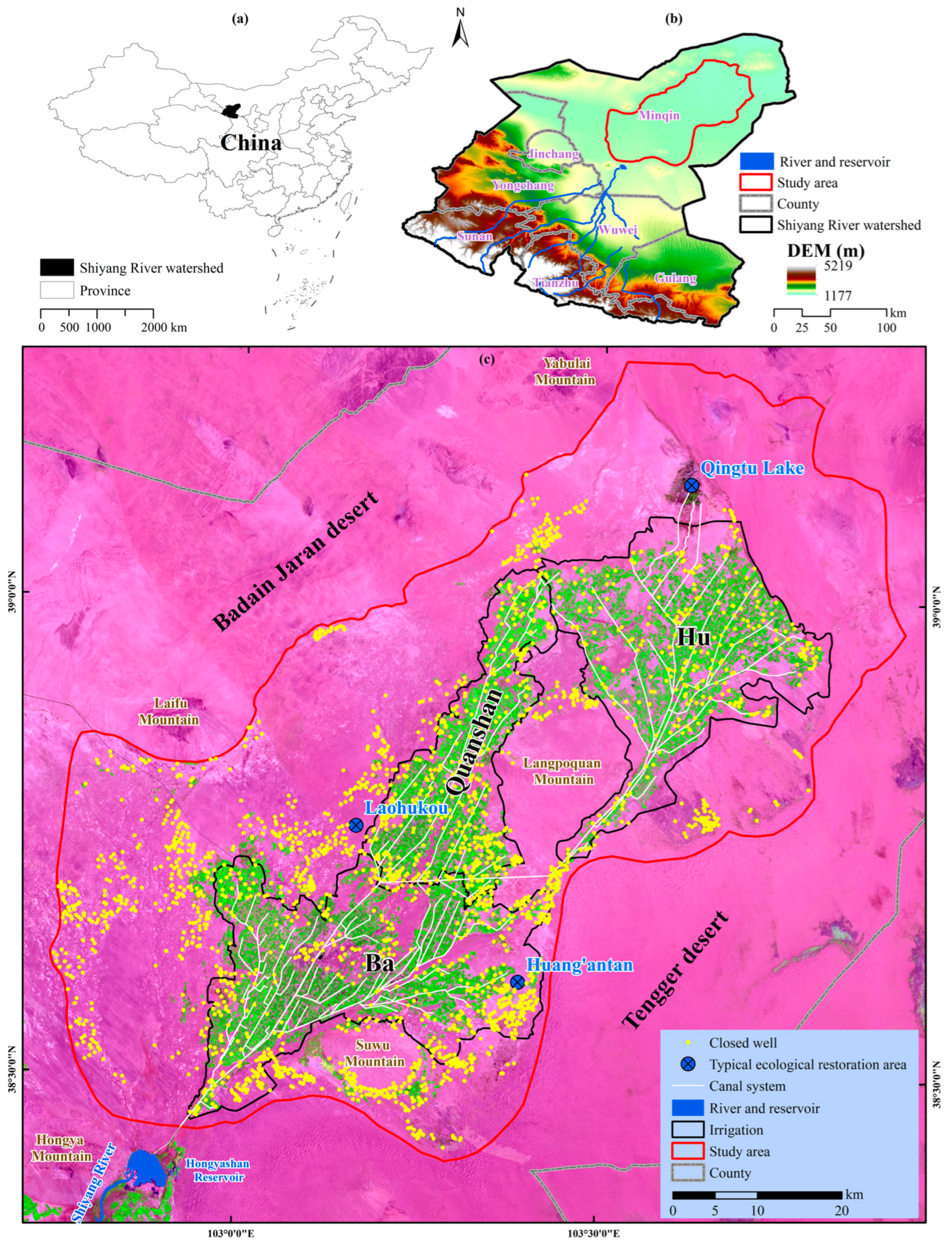
2.1. Study Area

The Minqin Basin is situated in the lower reaches of the Shiyang River watershed in the arid interior of northwest China (38°24′–39°15′ N, 102°40′–103°55′ E). It is surrounded by the Badain Jaran and Tengger deserts and is characteristic of desert–oasis ecosystems, with an inner oasis landscape (in this case, the irrigated regions of Ba, Quanshan, and Hu) and an outer desert (the periphery of the irrigated regions) (Figure 1). It has attracted worldwide attention as an important part of the ecologically sensitive region because of its role as a barrier to desertification. The study area has an area of 5200 km² and a temperate continental arid climate with dryness and little precipitation (114 mm/year) and strong evaporation (2483 mm/year). The average annual temperature is 8.4 °C, and the mean annual wind speed is 2.7 m/s. The cultivated areas without surface runoff are irrigated with water from the Hongyashan Reservoir through a canal system or watered with groundwater from wells. There are three famous ecological restoration sites in the study region, namely Qingtu Lake, Huang’antan, and Laohukou. Qingtu Lake is the endorheic or terminal lake of the Shiyang River, which completely dried up in 1959 but gradually became a wetland from 2010 through increased water arrival from the implementation of the CTSRB. Huang’antan is also a system of regenerating wetlands, which were gradually formed due to artesian wells (groundwater level rises) following the implementation of the CTSRB. Laohukou is a large area of artificial forests of mostly Haloxylon ammodendron and is characteristic of plantations used as windbreaks and for sand fixation in western China.

2.2. The CTSRB

Increasing human activities have caused a decline in the water supply through the over-exploitation of groundwater resources. Excessive irrigation and water waste have caused a series of serious ecological and environmental problems, such as a decline in groundwater level, vegetation degradation, desertification, and salinization [38,40,41]. To control the continuous decline in groundwater level in the Minqin Basin and to repair the seriously degraded Shiyang River Basin ecosystem, the Chinese government launched the Comprehensive Treatment Program of the Shiyang River Basin (CTSRB) in January 2006. It aimed to increase the surface water supply and reduce groundwater mining through a series of ecological restoration measures such as adjustments to the structure of the planting industry (e.g., increasing the planting proportion of low-water-consumption cash crops while reducing the proportion of high-water-consumption food crops, vigorously developing the labor economy, and facilitating agriculture), enforcement of water resource allocations and guarantees, water-saving irrigation efficiency projects (e.g., repairing the lining of canals, upgrading in-field irrigation patterns, and promoting water-saving agronomic techniques), ecological construction and protection projects (e.g., tree planting, ecomigration, and new energy construction in rural areas such as solar energy and biogas), water resource protection initiatives, management system construction (e.g., farmers’ water user association and water resource dispatching management information systems), and so on. The unofficial goal was to prevent Minqin from following the fate of Lop Nor, a former saltlake in western China. The CTSRB was divided into two parts, CTSRB I, an initiation period from 2006–2010, and CTSRB II, the implementation period which was initially supposed to last from 2011–2020. In December 2011, the National Development and Reform Commission and the Ministry of Water Resources shorten the CTSRB II period to 2015 according to the progress of the CTSRB to further accelerate the pace of governance in the Shiyang River Basin and engage in additional activities deemed necessary during the new scheduled duration of CTSRB II (2011–2015).

2.3. Data and Methods

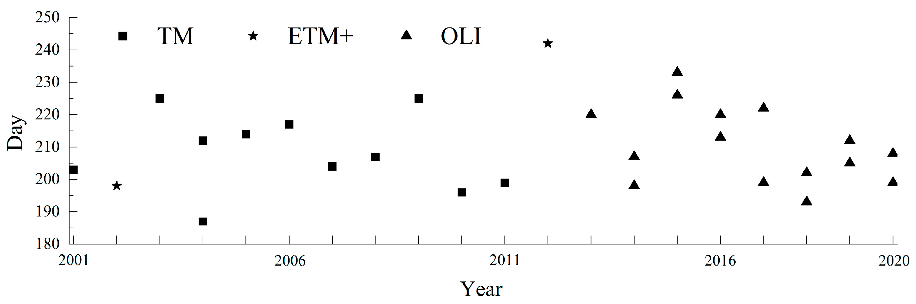
2.3.1. Data

The data in this study mainly consist of Landsat images downloaded from USGS (http://glovis.usgs.gov/, accessed on 2 March 2023) covering the time interval from 2001 to 2020. For each year, images were taken from July to August when vegetation grows peaks. They have a spatial resolution of 30 m and a total of 28 scenes over 20 years (Figure 2). We preprocessed the images using radiometric calibration, atmospheric correction, and image mosaicking and clipping to reduce differences between the sensors of Landsat. Additionally, we acquired precipitation and evaporation data from the China meteorological data system (https://data.cma.cn/, accessed on 26 April 2023), socio-economic and water resource data from the statistical yearbook of Minqin County, and data on pump wells from the Water Resources Bureau of Minqin.

2.3.2. Data Processing and Statistical Analysis

We reconstructed the spatiotemporal distribution of vegetation growth for each pixel–year using a standard remote sensing inversion method. To do so, we calculated the GDVI (see Equation (1) [42]), as this index has been shown to be superior in arid regions compared to other vegetation growth indicators such as the normalized difference vegetation index (NDVI) [42,43,44,45]. In addition, the GDVI is based on red and near-infrared bands and often contains more than 90% of the information relating to vegetation [46], and for Landsat data, its prediction of vegetation growth is the most accurate, with it being superior to other bands such as green, blue, and/or shortwave infrared bands [47].

$$GDVI=\frac{{{\rho }_{nir}}^2-{{\rho }_{red}}^2}{{{\rho }_{nir}}^2+{{\rho }_{red}}^2}$$

(1)

where ${\rho }_{nir}$ and ${\rho }_{red}$ are the near-infrared and red light bands of Landsat images, respectively.

We used the mean GDVI values and the area of different GDVI ranges to characterize the spatiotemporal variability of vegetation growth in the Minqin Basin. The mean value was calculated by averaging the GDVI values of all pixels. The area was defined as the area of GDVI at each 0.2 interval. Spatial and temporal heterogeneities were also taken into consideration. We analyzed these two indices for six different spatial divisions of the study area: the entire study area, the entire irrigated extent of the study region, the entire non-irrigated extent of the study region, and the three districts that together defined the full extent of the irrigated area (Figure 1).

We divided the time series into four equal-duration divisions based on the implementation of the CTSRB. The first was the pre-CTSRB period from 2001 to 2005, which predated the initiation of the restoration initiative. Next came the CTSRB I period (2006–2010), marking the project initiation phase. The final two time divisions were the CTSRB II period (2011–2015), when many of the restoration activities were implemented, and the post-CTSRB period (2016–2020) after the project was completed. For each of the four periods, we calculated the trend in vegetation growth through time and the stability of growth in space.

We analyzed the trend in values using trend line analysis (TLA). TLA, also known as linear propensity estimation, is a method to estimate upward or downward tendencies of data in a time series, changes in spatial distribution patterns, and turning points or mutations at certain moments of serial data using least-squares regression. This method is effective at characterizing variation in the trend of each phase of a time series, in this case reflecting the spatial variation characteristics of vegetation growth in different periods. TLA is calculated according to the following formula [48]:

$${\theta }_{slope}=\frac{n\times \sum _{j=1}^{n}j\times {GDVI}_j-\sum _{j=1}^{n}j\sum _{j=1}^n{GDVI}_j}{n\times \sum _{j=1}^n{j}^2-{\left(\sum _{j=1}^{n}j\right)}^2}$$

(2)

where ${\theta }_{slope}$ is the slope of the trend line; n is the cumulative number of monitoring years; and ${GDVI}_j$ is the GDVI value of each pixel in the jth year. A positive value indicates an increasing trend of the GDVI in a given time period (i.e., increasing plant growth), while a negative value means the reverse.

According to the value of ${\theta }_{slope}$, the change in vegetation growth is divided into six types [49,50] (

Table 1. Grade standard of vegetation growth changes in the Minqin basin.

Grade	Types	Classification Standard
I	obvious degradation	≤−0.010
II	moderate degradation	(−0.010, −0.005]
III	mild degradation	(−0.005, 0.000]
IV	mild improvement	(0.000, 0.005]
V	moderate improvement	(0.005, 0.010]
VI	obvious improvement	>0.010

) to analyze the ecological restoration effect of the CTSRB.

Stability was measured by calculating coefficients of variation (Cv). Cv is the ratio of the standard deviation (SD) to the mean and reflects the dispersion of a dataset. We calculated Cv according to the following formula:

$$\mathsf{\delta }=\sqrt{\frac{{\sum }_{j=1}^n{({GDVI}_j-\overline{GDVI})}^2}{n}}$$

(3)

$$Cv=\frac{\delta }{\overline{GDVI}}$$

(4)

where $\delta$ is SD; n and GDVI_j are the same as Equation (2); and $\overline{GDVI}$ is the average value of the multi-year GDVI. The larger the Cv is, the farther the GDVI value of pixels in the time series is from the mean and the greater the interannual variation in the GDVI, which indicates lower stability in vegetation growth.

3. Results

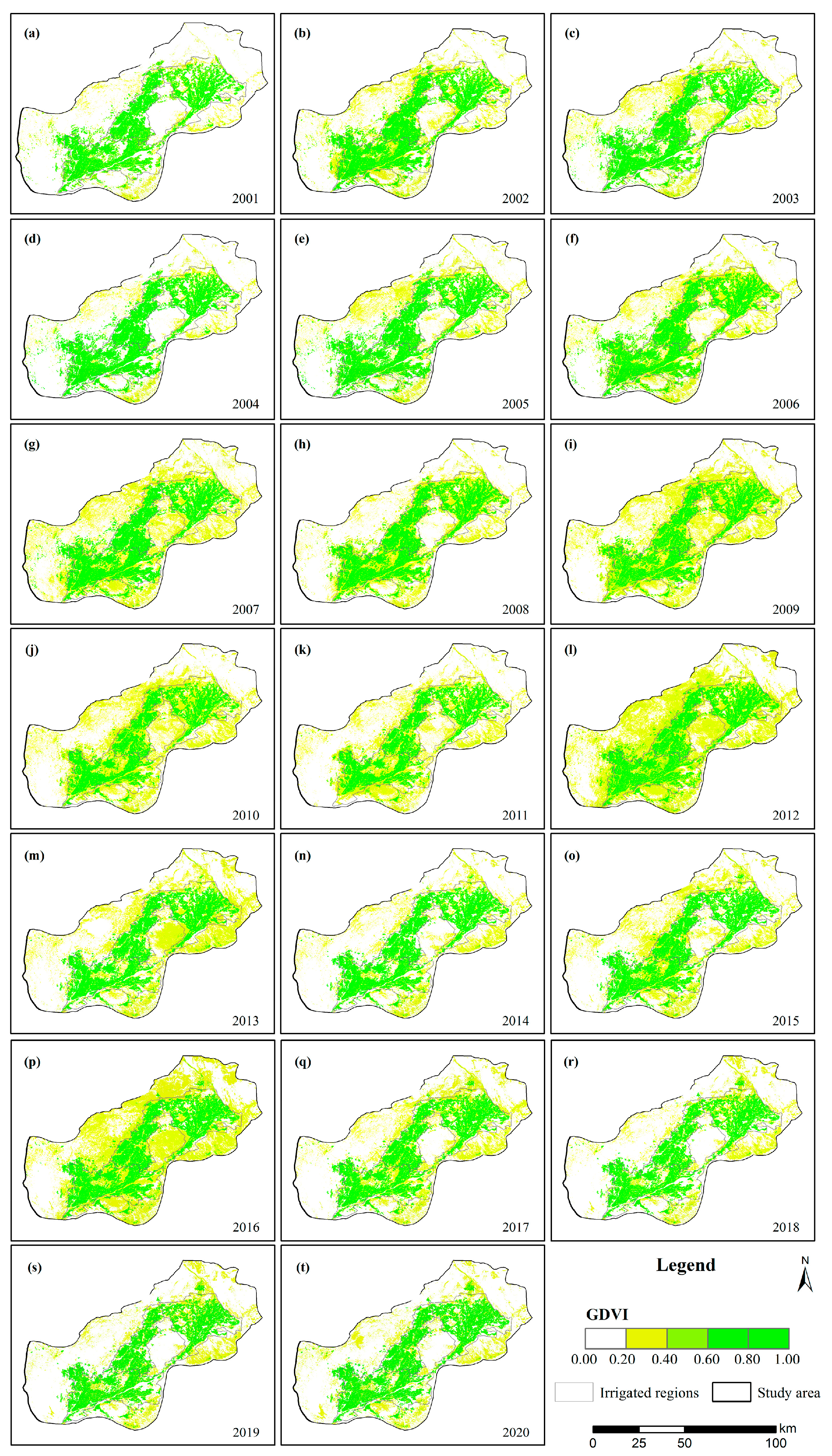
3.1. The Spatiotemporal Distribution of Vegetation Growth

We found that vegetation growth displayed significant spatial and temporal heterogeneities not only within and along the periphery of the irrigated regions but also between the three separate irrigated regions (Figure 3). Unsurprisingly, vegetation growth within the irrigated region was higher than in the desert areas at the periphery of the study region, which is typical of the vegetation distribution in desert–oasis ecosystems. The vegetation growth changed significantly before and after the implementation of the CTSRB in the Shiyang River Basin. During the pre-CTSRB period (2001–2005), the areas with GDVI > 0.6 at the periphery of the irrigated regions were mainly cultivated vegetation (crops) for agricultural development. During the CTSRB I period, with the implementation of ecological restoration measures in the form of a “close the pumping-wells, transform the land” strategy, the cultivated vegetation at the periphery of the irrigated regions was gradually abandoned (for natural restoration) or replaced by vegetation planted for restoration purposes (Haloxylon ammodendron plantations for wind and sand management), and the area with GDVI > 0.6 was gradually reduced, especially in 2008. During the CTSRB II and post-CTSRB periods, the vegetation growth at the periphery of the irrigated regions improved, and naturally vegetated areas (Qingtu Lake and Huang’antan) with GDVI > 0.6 appeared, and the area gradually expanded. The years of 2012 and 2016 were the best years for vegetation growth at the periphery of the irrigated regions across the entire 20-year dataset.

3.2. Changes in Vegetation Growth before and after the Implementation of the CTSRB

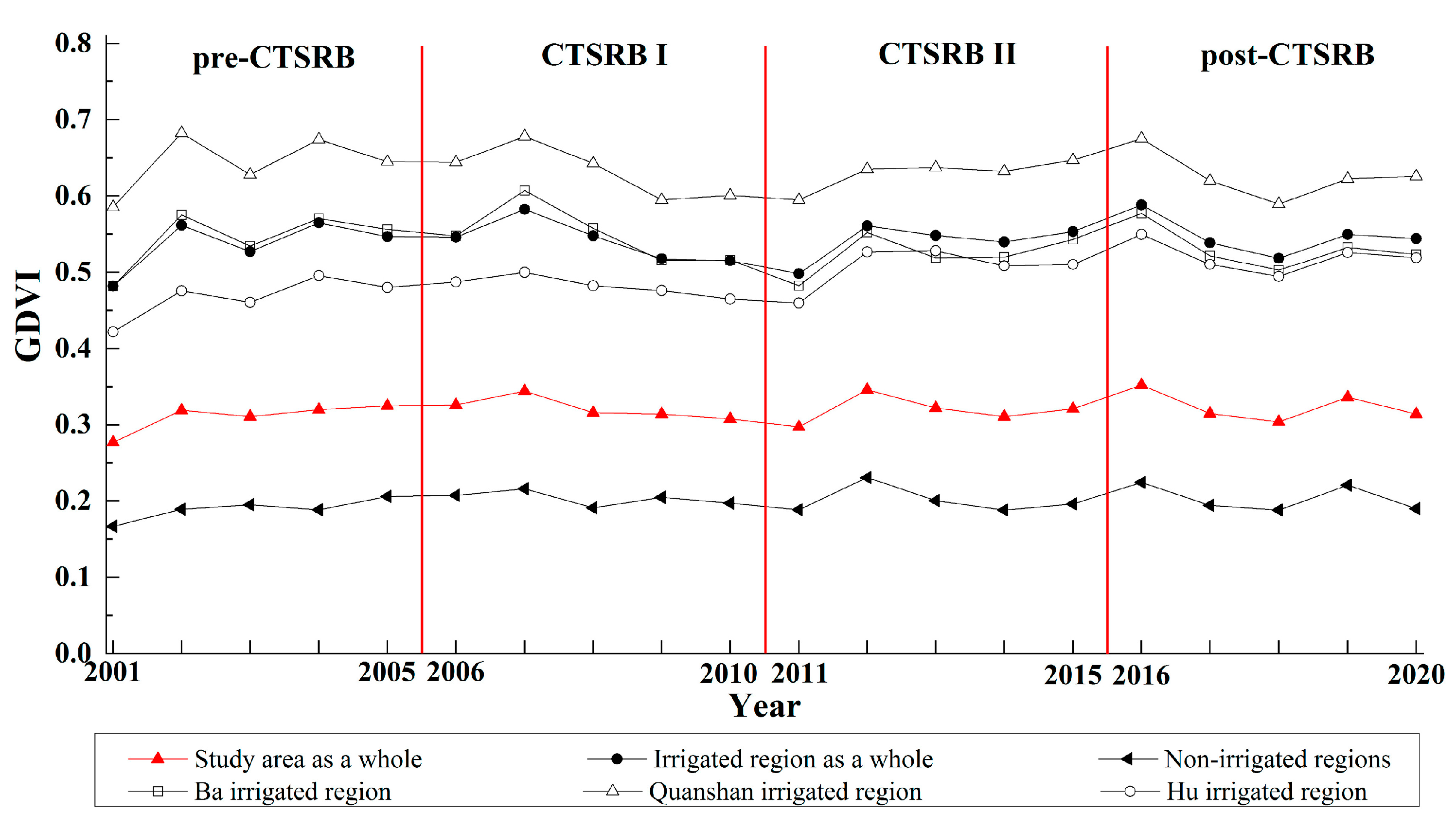
3.2.1. Mean Value Changes

The mean values of the GDVI in the six regions from 2001 to 2020 are shown in Figure 4. Slight increases were detected during the pre-CTSRB period. For the entire study area, the GDVI increased from 0.277 to 0.325 at the rate of 0.012/year. The vegetation growth within and outside of the irrigated regions increased from 0.482 and 0.167 to 0.547 and 0.206, respectively, at the rate of 0.016/year and 0.010/year, respectively. For the three irrigated sub-regions, the rates of increase were not obviously different, with a rate of 0.019/year in Ba, 0.015/year in Quanshan and 0.014/year in Hu. The mean values increased from 0.481, 0.586 and 0.422 to 0.556, 0.645 and 0.480, respectively. Hu showed the greatest increase in the GDVI among the six regions.

In the CTSRB I period, the GDVI increased initially from 2006 to 2007 but began to decline afterward. The study area as a whole averaged a decline of 0.05/year during the CTSRB I period. This was primarily driven by the decline in the GDVI within the irrigated regions, which decreased from 0.546 in 2006 to 0.515 in 2010 at the rate of 0.008/year, three times the rate at the periphery of the irrigated regions. For the three irrigated regions, the rates of decline differed obviously from each other. Ba had the fastest rate of decline at 1.32/year, dropping to 0.482 by 2010; Quanshan declined from 0.644 to 0.595 at an intermediate rate of 0.98/year; and the slowest rate of decline was observed in Hu, where the GDVI to 0.460 in 2011 at a rate of 0.55/year. The GDVI of all six regions showed a downward trend, and for four regions (the entire study area, the whole irrigated region, Ba, and Quanshan), the decline was greater than the increase observed during the pre-CTSRB period.

In the first half of the CTSRB II period (2011–2014), the mean values of the GDVI in the six regions increased initially but subsequently decreased before gradually increasing after 2014. By 2016, the last year of our study period, the GDVI of the study area as a whole and outside of the irrigated regions was 0.352 and 0.224, respectively. The growth rate of both regions was less than or equal to 1.10/year. In contrast, the GDVI means for Ba, Quanshan, and Hu, increased rapidly at a rate of 1.80/year, 1.90/year, 1.61/year, and 1.80/year, respectively. In 2016, all three values were above 0.55, with the highest value of 0.675 observed in Quanshan. The GDVI of all six regions showed an increasing trend during the CTSRB II period, and the increasing range was smaller than the decreasing range in the CTSRB I period.

The GDVI fluctuations during the post-CTSRB period exhibited nearly the opposite pattern of the CTSRB II period. The GDVI first decreased, then increased, and then decreased slightly. In 2020, the GDVI of the entire study area and of the irrigated and non-irrigated regions were 0.314, 0.544, and 0.190, respectively, with average annual changes of −0.95%/year, −1.10/year, and −0.86%/year, respectively. For the three irrigated regions, the decline rate was greatest in Ba, followed by Quanshan, and then Hu, and the GDVI in 2020 was 0.524, 0.626, and 0.519, respectively. As far as the variation range was concerned, the entire study area was basically the same as that in the CTSRB II period. The variation range at the periphery of the irrigated regions was twice that of the CTSRB II period. The variation range of the other four regions was narrower than that of the CTSRB II period.

Looking at the entire study period, the mean values of the GDVI in the end year (2020) of the six regions were all greater than those in the start year (2001). Hu had the largest annualized rate of change of 0.51/year. The irrigated region as a whole increased by 0.33/year. The difference in the rate of increase was not significant between Ba and Quanshan, and both were less than half of Hu. The study area as a whole increased 0.0019/year. The non-irrigated region showed the smallest annualized increase of 0.12/year.

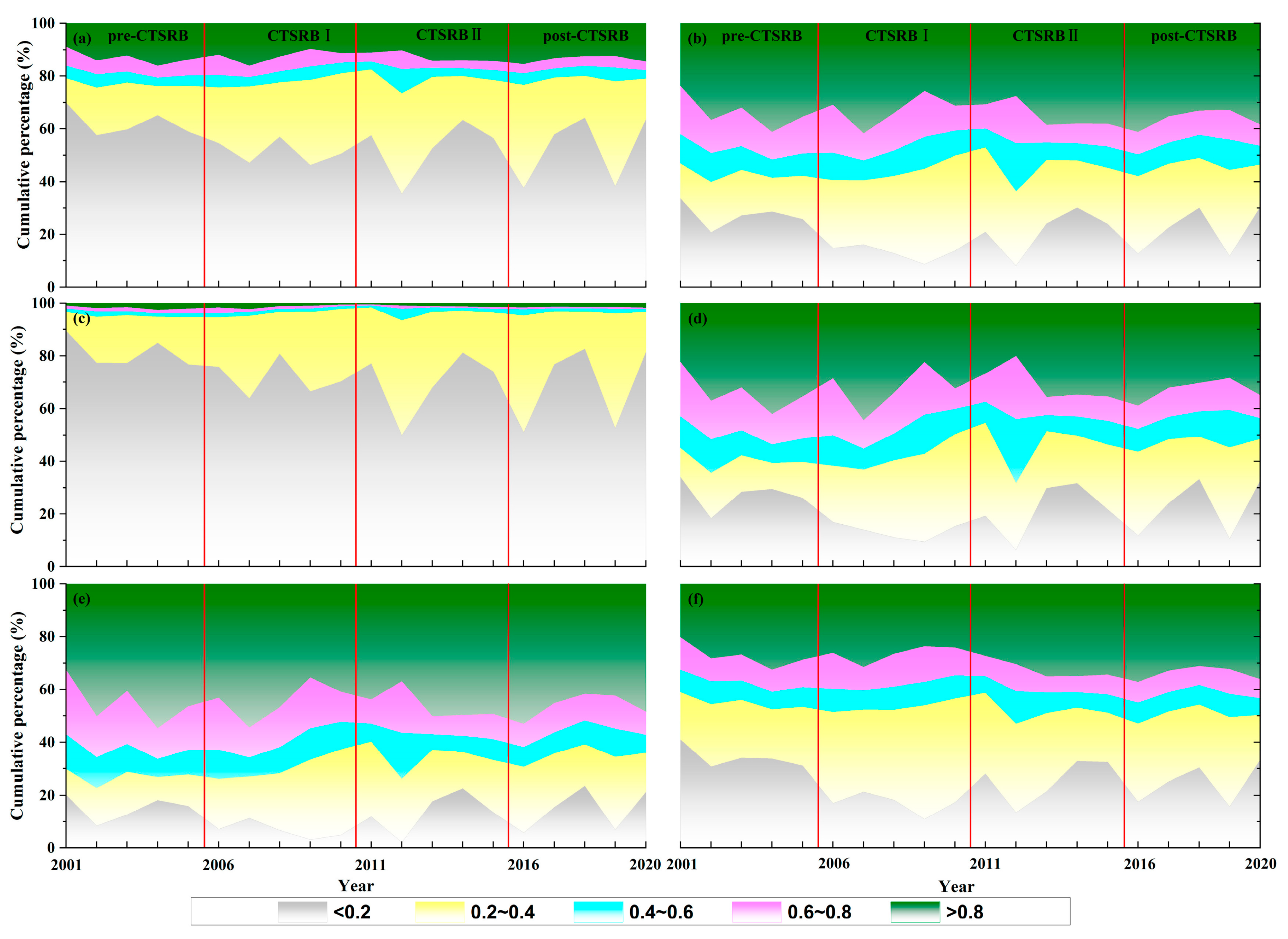
3.2.2. Cumulative Distributions of GDVI Values

The high interannual variability of plant growth in the study region over the study period is further underscored by the fluctuating distribution of the GDVI through time (Figure 5). After binning the data into bands of 0.2 units of the GDVI, the cumulative area with a GDVI between 0 and 0.2 and between 0.2 and 0.4 showed the highest magnitudes of change, which was driven by high magnitudes of interannual change in the irrigated sub-regions (Figure 5b) but even more so in the non-irrigated region (Figure 5c), where such areas made up the vast majority of the total area each year.

During the second half of the study period (CTSRB II and post-CTSRB), the proportion of the study region with the lowest levels of plant growth (>0.2 GDVI) was significantly smaller than during the pre-CTSRB period, driven in large parts by large shifts in the cumulative area of the non-irrigated region that rose from <0.2 GDVI to between 0.2 and 0.4 GDVI, particularly in the years 2012, 2016, and 2019. Also during the second half of the study period, the proportion of area with a GDVI > 0.8 (which was found almost exclusively in the irrigated region) was higher on average than during the pre-CTSRB period (Figure 5b,c). This pattern was driven by the Ba and Hu irrigated subregions but was not the result of spikes in any given year (Figure 5d–f).

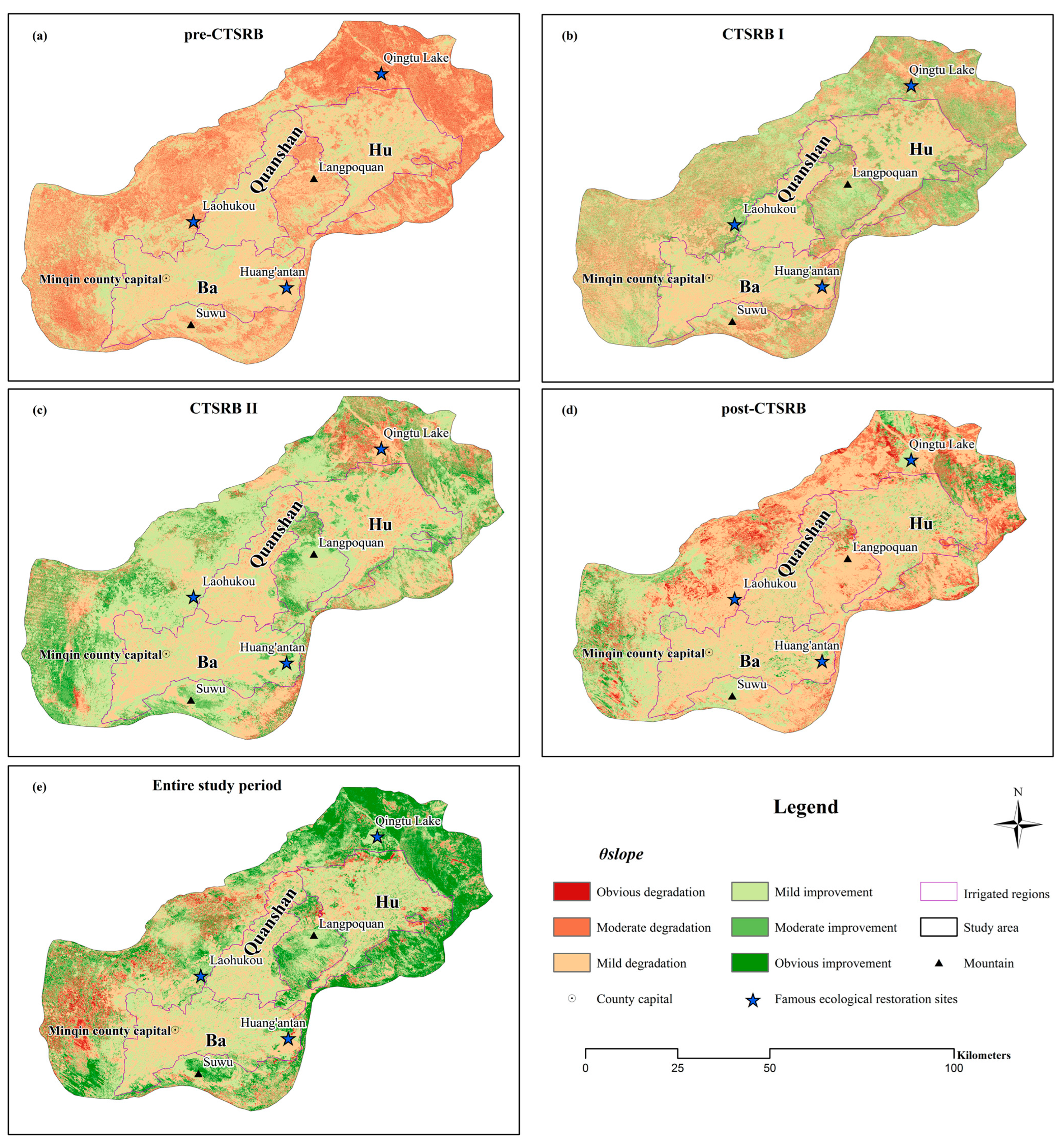
3.3. Vegetation Growth Trends

The highest magnitude trends in plant growth during the study period generally occurred outside the irrigated region (Figure 6). During the pre-CTSRB period, vegetation growth in large areas at the periphery of the irrigated regions declined, and the vegetation degraded obviously (Figure 6a). The irrigated region fared much better, with slightly positive GDVI trends, except for the east part of Ba and the northwest part of Hu, where the trend was also clearly negative. During the CTSRB I period, the vegetation growth at the periphery of the irrigated regions began to improve, and the vegetation recovered somewhat (Figure 6b). The periphery regions around Quanshan and Hu recovered more than in Ba. The situation for the irrigated region reversed during the pre-CTSRB period; the vegetation growth recovered significantly during this period in the eastern part of Ba and the northwestern part of Hu. During the CTSRB II period, the GDVI trends indicate strong plant recovery in Qingtu Lake and on denuded mountain slopes, especially Suwu Mountain and Langpoquan Mountain (Figure 6c). Large desert areas at the periphery of the irrigated regions further improved. The vegetation recovery around Ba was stronger than in Quanshan and Hu during this period. The trend in the GDVI in the area surrounding Qingtu Lake decreased while the vegetation growth in the irrigated region further recovered during this period. During the post-CTSRB period, the trends in the irrigated region were similar to the CTSRB II period (Figure 6d). Except that the vegetation in the southwest and northeast of the study area, most of the vegetation at the periphery of the irrigated regions degraded. From the perspective of the entire study period, the vegetation is largely in a state of recovery (Figure 6e). Except for a small amount of vegetation degradation in the west periphery of Ba, the vegetation outside of the irrigated areas showed a strong trend toward recovery, especially in the areas surrounding Hu.

The internal and external areas of Hu, Ba, and Quanshan exhibit spatial heterogeneity and temporal variability at different stages of the project. Using the slope of GDVI, the impact trend of spatiotemporal changes in vegetation growth on ecological restoration was depicted. Specifically, during the pre-CTSRB period, the area covered in degrading vegetation was as high as 77.28%, accounting for 2/3 of the entire study area (Figure 7a). The degradation was mainly mild or moderate, accounting for 52.76% and 20.25% of the area, respectively. During the CTSRB I period, vegetation degradation slowed, with 26.7% experiencing net degradation. Conversely, the areas of mild, moderate, and obvious improvement increased to 14.37%, 9.34% and 2.99%, respectively. During the CTSRB II period, degradation declined further, and the degraded area fell from 50.58% during the CTSRB I period to 36.27%. No areas showed signs of obvious degradation, and areas classified as undergoing moderate degradation made up just 5% of the study region. Close to two-thirds of the entire study area underwent vegetation growth, of which the areas with mild, moderate, and obvious improvement reached 45.99%, 11.69%, and 6.04%, respectively. During the pre-CTSRB period, the area experiencing degradation expanded to 66.78% of the study region, while only 26.50% showed mild improvement, and the areas of moderate and obvious improvement were only a third of the values of the CTSRB II period. Zooming out to the study period as a whole, 34.06% of the study region was classified as having improved mildly, making it the most common classification. Two-thirds of the study region showed some level of improvement, while only 28.99% showed degradation, most of which (23.99%) was mild.

In terms of the whole irrigated region (Figure 7b), vegetation growth was dominated by mild degradation and supplemented by a mild improvement. With the implementation of the CTSRB, the degradation trend was gradually curbed and the vegetation growth improved. During the pre-CTSRB period, the areas of mild, moderate, and obvious active degradation were 60.48%, 5.46%, and 0.90%, respectively. During the CTSRB I period, the areas of mild and moderate degeneration decreased by 8.65% and 2.28%, respectively, while the area of obvious degeneration increased by 0.04%. During the CTSRB II period, the degradation phenomenon was further alleviated, and the area of degradation decreased to half of the whole irrigated region, and the obvious degradation phenomenon was completely contained. During the post-CTSRB period, the area of degradation increased again, reaching 63.68%. The area of mild degradation mainly increased, while the area of moderate and obvious degradation remained basically unchanged (the increments were less than 1.00%). Across the entire study period, the area of net degradation was 40.31%, which was also dominated by mild degradation; moderate and obvious degradation accounted for less than 3.50% of the total area of the entire study region. On the other hand, the improvement in vegetation growth became more and more obvious. During the pre-CTSRB period, the area of mild improvement accounted for 32.30% of the irrigated subregions, while moderate and obvious improvement accounted for less than 1% of the area. During the CTSRB I period, the total irrigated area experienced some form of improvement, especially the areas of obvious and moderate improvement, which increased from 0.15% and 0.72% in the pre-CTSRB period to 1.54% and 5.56%, respectively, with maximum increases as high as 938.93% and 677.38%, respectively. During the CTSRB II period, there was a small reduction in the area of moderate and obvious improvement, but the area of mild improvement continued to increase. During the post-CTSRB, the areal extents of the three improvement classes all decreased to varying degrees. From the perspective of the entire study period, the area of mild improvement (48.36%) accounted for about half of the entire study area, which was four times the summed area of moderate and obvious improvement.

For the non-irrigated regions (Figure 7c), mild and moderate degradation were the main factors, accounting for 48.61% and 28.21% of the entire study area, respectively, during the pre-CTSRB period. Improving areas accounted for just 17.10%. During the CTSRB I period, vegetation growth improved substantially, with the area of mild improvement doubling to 34.18%, and the area of moderate and obvious improvement also increasing by 11.77% and 3.85%, respectively. The area of degradation decreased by 35.21%. During the CTSRB II period, improvements was more obvious, and the area of improvement reached 71.47%, more than 2/3 of the non-irrigated regions, of which the areas of moderate and obvious improvement increased to 15.62% and 8.67%, respectively. The obvious degradation of vegetation growth was completely curbed, the areas of mild and moderate degeneration were reduced to 1/2 and 1/5 of that in the pre-CTSRB period, respectively. During the post-CTSRB period, the vegetation degradation phenomenon worsened. The area of degradation (68.45%) was equivalent to the area of improvement in the CTSRB II period, and the areas of mild and moderate degradation were more than twice that in the CTSRB II period. The area of obvious degradation reached 5.23%. The areal extent of three improvement classes was less than half of the previous period. From the perspective of the entire study period, vegetation recovery was obvious, and the areas of mild, moderate, and obvious improvement were all about 25%. The area of mild degradation was 16.96%, and the summed areas of moderate and obvious degradation were about 1/10 of the non-irrigated regions.

For the three different irrigated regions (Figure 7d–f), during the pre-CTSRB period, the vegetation growth in Ba, Quanshan, and Hu was dominated by mild degradation and to a slightly lesser extent mild improvement. The area of mild degradation and mild improvement in Ba and Quanshan was more than 95% of each region and close to 90% in Hu. Mild degradation accounted for about twice as much area as mild improvement. During the CTSRB I period, the areal extents of mild, moderate, and obvious improvement in the three irrigated subregions all increased to varying degrees. Except for the area of obvious degradation in Ba, which increased by 0.22%, the area of mild, moderate and obvious degradation decreased slightly. During the CTSRB II period, the obvious degradation phenomenon in the three irrigated regions was completely contained, and the moderate degradation phenomenon in Ba was further slowed down, and the degraded area was less than 1%. The moderate degradation phenomenon in Quanshan and Hu rebounded. The area of moderate degradation in Quanshan and Ba was 3.78% and 5.02%, respectively, which in Quanshan was higher than the previous two periods and in Ba was between the levels of the pre-CTSRB and CTSRB I periods. The mild degradation phenomenon was further slowed down, and the mild improvement phenomenon recovered further in the three irrigated regions, until the areas of mild degradation and mild improvement were equivalent. The trend of moderate and obvious improvement slowed down, and the area was smaller than that of the CTSRB I period but higher than that of the pre-CTSRB period. During the post-CTSRB period, areas undergoing degradation in the three irrigated regions increased and accounted for a similar proportion (62.36~64.92%). The area of moderate and obvious degradation in Quanshan was twice that of Ba, and the area of moderate and obvious degradation in Hu was the largest among the three irrigated regions, accounting for 6.52% and 1.19%, respectively. The area of mild improvement was equivalent to that of the three irrigated regions (31.43~32.68%), moderate (less than 1.50%) and obvious improvement (1.92~3.49%). In each case, the extent for Hu was greater than Quanshan, which was greater than it was for Ba. For the entire study period, the area of vegetation improvement (55.25~66.06%) in the three irrigated regions was larger than the areal extent undergoing degradation. Among them, the area of mild improvement accounted for half of the improved area. The area of mild degradation was the smallest in Hu, accounting for 28.09%, while for Quanshan and Ba, it accounted for 40.83% and 43.25%, respectively. The areas of moderate improvement and moderate degradation followed the pattern of Hu (12.36%, 4.10%) > Quanshan (7.12%, 1.86%) > Ba (5.80%, 1.28%). The areas of obvious improvement and obvious degradation were both the largest in Hu, and both were close to 5%. For both Ba and Quanshan, obvious improvement and degradation were less than 2.00% and 0.20%, respectively.

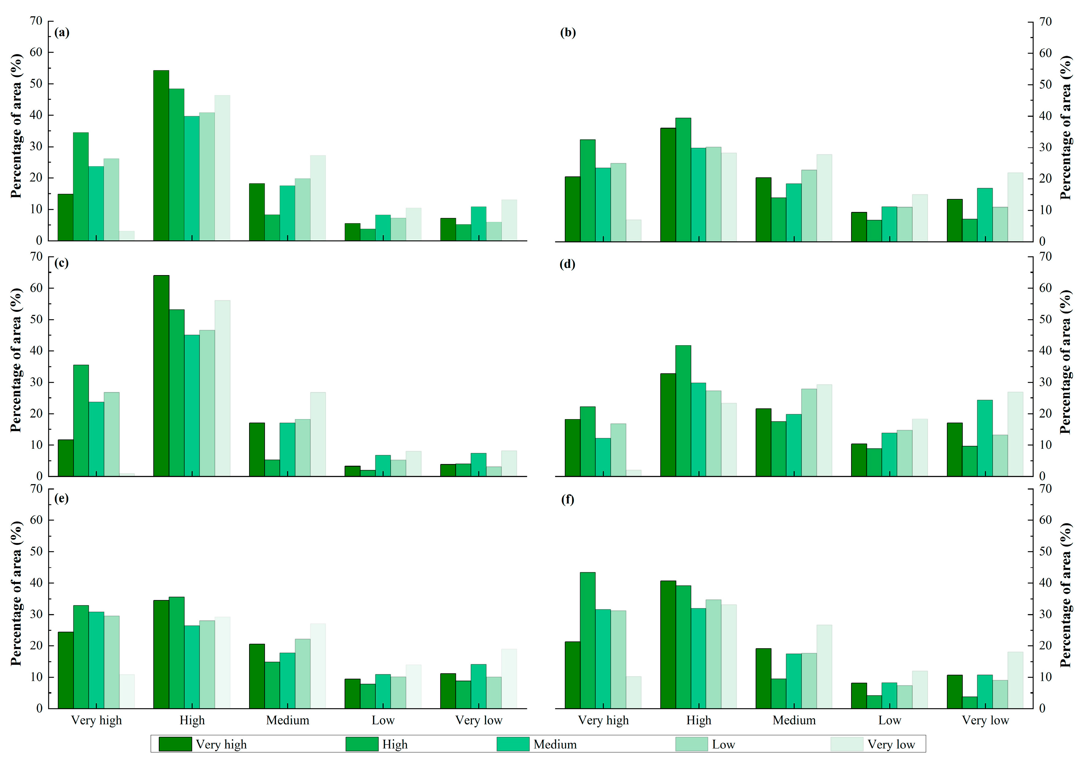
3.4. Vegetation Growth Stability

The stability of the GDVI in each study period showed strong spatiotemporal heterogeneity (Figure 8). During the pre-CTSRB period, high and medium stability characterized the GDVI for large swaths of the non-irrigated regions (Figure 8a). Areas of low and very low stability were mainly distributed around Ba and the newly cultivated farmland at the periphery of the irrigated regions, which caused the speckled pattern in Hu as high salinity of the soil led to cropping changes or land abandonment. During the CTSRB I period, very high stability characterized much of the area at the periphery of the irrigated regions, and very low stability areas were mainly located near closed wells (Figure 8b). By the CTSRB II period, the regions of low and very low stability expanded significantly except for around the periphery of Hu (where the stability was still very high). The regions of low stability were mainly located at the edge of the desert in the north and west of Ba, northwest of Quanshan near the road through the Badain Jaran Desert, inside Hu (still speckled), and in the Qingtu Lake, Huang’antan, and Laohukou regions (Figure 8c). During the post-CTSRB period, the area marked by high stability was greatly reduced, and the vast majority of the regions were very low and or of medium stability (Figure 8d). Throughout the entire study period, vegetation stability was very poor, with few regions classified as very high stability. The extent of low and very low stability areas was basically consistent with those of in the CTSRB II period but spread more broadly (Figure 8e).

From the perspective of the entire study area (Figure 9a), during the pre-CTSRB period, areas with high and very high vegetation stabilities made up close to 70.00% of the entire study area. Low and very low areas were 7.19% and 5.42%, respectively. By the CTSRB I period, high stability areas reached 34.44%, increasing by nearly 20.00%. High and medium areas decreased by 6% and 10%, respectively, while low and very low areas both decreased by 2.00%. During the CTSRB II period, the vegetation stability was worse than that in the previous period. High and very high areas both decreased by 1/10, while medium areas increased by 1/10. Low and very low areas increased by 5.00%, respectively. Stability improved slightly during the post-CTSR period: high, very high and medium areas all increased slightly (<3.00%), while the low and very low areas were opposite those of the pre-CTSRB period, decreasing by 1.04% and 4.84% compared with the CTSRB II period, respectively. Throughout the entire study period, areas of high stability dominated (46.35%), followed by medium stability areas (27.16%); both low and very low stability were 11.00%; very high stability only accounted for 3.03%.

In terms of the whole irrigated region (Figure 9b), the vegetation stability was mostly high, followed by very high and medium, and the three totaled >70.00% in the four study periods. Areas of high and very high stability were 36.11% and 20.70% in the pre-CTSRB period, respectively, and increased to 39.47% and 32.44% in the CTSRB I period, respectively, decreased by 10% in the CTSRB II period, and then slightly increased (<1.50%) in the post-CTSRB period. After decreasing in the CTSRB I period, the area of medium stability gradually increased in the latter two periods, with it reaching 22.84%. Low and very low areas were at their least extensive and equivalent to their values in the CTSRB I period, and both were at their largest in the CTSRB II period, with them accounting for 17.04% and 11.11%, respectively, and about 10.00% in other periods. From the perspective of the entire study period, medium areas were 27.79%, high and very high areas were equivalent to low and very low areas, both around 35.00%, of which high areas (28.29%) were about equal in extent to medium areas, and very high areas made up about 7.00% of the total. Low areas were twice that of very high and 3/4 that of very low stability areas.

For non-irrigated regions (Figure 9c), the high stability areas were most common (>45.05%) and changed in a “V” shape, that is, from a maximum in the pre-CTSRB period (64.07%), down in the CTSRB I period (53.22%), and again to a minimum in the CTSRB II period (45.05%) before gradually recovering in the post-CTSRB period (46.58%) (Figure 7c). The medium area also showed a “V” shape change, but the trough was in the CTSRB I period (5.28%), and the extent was the same before and after the implementation of the CTSRB. Very high stability areas increased from 11.73% (pre-CTSRB) to 35.52% (CTSRB I), decreased by 11.77% (CTSRB II), and reached 26.81% in the post-CTSRB period. Very low areas were greatest in extent during the CTSRB II period (7.39%) and were around 3.50% in the other periods. Low areas were 1, 0.5, 1, and 1.5 times that of the very low areas for the four time periods. Across the entire study period, high stability areas made up 56.06% of the study region, which was 30 percentage points more than the extent of medium stability areas. Low and very low areas were both 8% of the total, and very high areas were less than 1%.

For the three different irrigated subregions (Figure 9d–f), the four periods were dominated by high stability. Except for the CTSRB I period, the high stability extent of Ba and Quanshan was not significantly different in each period. Hu’s high stability extent was 5 percentage points more than the other two irrigated regions in each period. Very high and medium stability areas were the next most common, and both changed greatly in the two periods of the CTSRB, but the area was similar in the pre-CTSRB and post-CTSRB periods (except for very high areas in Hu). The area of very high stability decreased with the gradual implementation of the CTSRB, while the medium area increased in contrast. Very low areas were slightly more extensive than low areas in each period, and the difference was largest in the CTSRB II (the maximum difference was 10.46%) and pre-CTSRB periods (the maximum difference was 6.61%), and smaller in the CTSRB I (<1.00%) and post-CTSRB periods (≤1.65%). For Ba, across the entire study period, medium areas were most extensive (29.29%), followed by very low areas (26.92%). Very high areas were the least common at only 2.03%. In Quanshan, high areas made up close to 30% of the total, low and very low areas were about 15%, while very high areas accounted for 1/10 of the total. Areas of high stability in Hu made up 33.17%, low areas were about 1/10, and the proportions of other levels were not different from those in Quanshan. By analyzing the trends in and stability of the GDVI and comparing various periods of the CTSRB, the differences in vegetation growth at different locations and time points within the study area were determined. It was found that the project gradually showed a significant positive impact on vegetation growth over time, indicating that the plan has achieved good results in improving the ecological environment, at least in vegetation diversity restoration.

4. Discussion

Water availability is one of the main drivers of vegetation growth in arid and semi-arid areas [51,52]. For the portions of the study area without surface runoff (surface water inflow depends on the discharge of the Hongyashan Reservoir, which is mainly used for irrigation), precipitation and groundwater are the key factors affecting the growth of natural vegetation. The precipitation in the first 5 days, the first 10 days, and the first 15 days of the selected images (Figure 10a) show that the precipitation in the previous period of the selected images in most of the years was below 30 mm, and for most of them, it was less than 10 mm, except for 2004 which had more precipitation (>40 mm) in the early stage. Therefore, we believe that the selected images are accurate representations of the vegetation growth in the study area for that year, and our results reflect the true vegetation growth in the Minqin Basin.

Overexploitation of water resources has led to severe ecological degradation and even desertification in some arid inland river basins in northwestern China [53], including the Shiyang River watershed [54,55,56]. Over our study period, both precipitation and evaporation in the study area showed a decreasing trend, but the rate of precipitation to evaporation showed an increasing trend (Figure 10b). Runoff increased, and the exploitation of groundwater decreased (Figure 10c), causing groundwater levels to gradually recover and stabilize [55]. The population also gradually decreased, and agricultural acreage first increased (pre-CTSRB period) and then decreased (CTSRB I period) before increasing again (CTSRB II and post-CTSRB periods) (Figure 10d). In general, water resource reserves increased and pressure on water supplies decreased after the implementation of the CTSRB. In addition, the implementation of water-saving irrigation measures gradually allowed more water to reach downstream natural systems (Figure 10e), which created favorable conditions for vegetation restoration in the study area. Additionally, the gradual implementation of ecological restoration projects, involving artificial windbreaks or tarps/other barriers to stop windblown sand or advancing dunes (Figure 8f), also slowed the pace of vegetation degradation in the study area, improving vegetation growth. Human beings have never lacked the perseverance and determination to engineer their environment for their benefit. These ecological restoration measures (especially artificial afforestation and sealing sand for afforestation/grass) have not been going on continuously since records began in 1950, but the effect was far less obvious than during the implementation of the CTSRB, suggesting that the groundwater level restoration plan may have been the more important component of the CTSRB.

Vegetation growth in the study area exhibited temporal and spatial heterogeneity from 2001 to 2020. This heterogeneity is likely determined by idiosyncratic ecosystem attributes and habitat characteristics. The difference is not obvious among irrigated regions, but it is obvious between the irrigated and non-irrigated regions. The artificial oasis area inside the irrigated region is significantly richer in plant growth than the desert area at the periphery of the irrigated regions as is typically the case for desert–oasis ecosystems. During the pre-CTSRB period, due to continuous reclamation and cultivation, a large amount of wasteland was reclaimed into cultivated land, so the mean values of the GDVI in the six regions slowly increased. During the CTSRB I period, water management reduced the area of the artificially cultivated oasis (48 km² of cultivated land was transformed), which reduced the mean values of the GDVI for the study region as a whole during this period. The effect of vegetation restoration was not obvious, but even a net trend of degradation in plant growth can still mark progress toward the restoration of natural vegetation at the periphery of the irrigated regions. During the CTSRB II period, due to the gradual rise in groundwater levels, the gradual growth of Haloxylon ammodendron plantations, and natural vegetation regeneration, combined with the gradual effect of ecological restoration projects such as engineering sand suppression, artificial afforestation, sealing sand for afforestation/grass, and other measures, the vegetation, especially the natural vegetation, showed clear signs of recovery. Unvegetated areas at the periphery of the irrigated regions gradually transformed to vegetated areas, and the growth of desert plants gradually improved. During the post-CTSRB period, due to the early completion of the CTSRB, funds used for ecological restoration activities were greatly reduced (the total investment in the CTSRB was 4.75 billion yuan). The attention paid by the government and public also decreased, and the rate of vegetation restoration slowed, with some areas becoming degraded again. From a comprehensive view, the restoration effect of the CTSRB on vegetation, especially natural vegetation in the Minqin Basin, cannot be ignored. The comprehensive management of water resources at the basin scale and multi-effect ecological restoration measures were the main reasons for the restoration of vegetation in the study area.

Closing wells was the main measure taken during the CTSRB I period, with a total of 2323 wells shuttered (Figure 1), resulting in 48 km² of cultivated land being transformed. To examine how the well closures affected vegetation recovery, we calculated the distances from the closed pumping wells (D_well) to the surrounding landscape and averaged the GDVI at intervals of 200 m. We compared the study region not affected by well closure (or rather the entire study area, since the 2323 pixels with closed pumping wells were insignificant compared with the 5,696,728 pixels in the whole study area) to the areas around the closed wells before and after the implementation of the CTSRB (Figure 11).

We found that the trends in and stability of the GDVI in the area around the closed wells was lower than the average for the study region as a whole (Figure 8b and Figure 11a). As D_well increased, the stability and trend in the GDVI gradually approached the average for the study region. On average, all D_well bins were undergoing active degradation, with the degree of that degradation varying greatly in the pre-CTSRB period. During the CTSRB I period, for areas where D_well ≤ 400 m, the GDVI trends were higher between 200 and 400 m from a closed well than they were for < 200 m from a closed well. At greater D_well, the degree of restoration increases and gradually plateaus. During the CTSRB II period, the degree of restoration increased with increasing D_well. The degree of degradation was not significantly related to D_well in the post-CTSRB period. Across the entire study period, vegetation underwent degradation when it was very near the wells that were closed during the study period, but the degree of degradation decreased with increasing D_well when D_well ≤ 200 m, after which the trend in the GDVI turned positive and gradually increased when D_well > 200 m. As for stability (Figure 11b), it increased with the increase in D_well in each period, meaning that the closer an area was to a closed well, the worse the vegetation stability was. This difference was obvious in the CTSRB I period and across the entire study period but not in the post-CTSRB period. Another interesting finding is that the smaller the D_well, the larger the mean values of the GDVI and the better the vegetation growth (Figure 11c). The inflection point appears at D_well = 1000 m. When D_well > 1000 m, vegetation growth was higher compared with 800 m < D_well ≤ 1000 m. Beyond that distance from the wells, the GDVI remained stable, independent of the distance, at least out to 1600 m, the maximum D_well we examined. In terms of time series, before the implementation of the CTSRB (i.e., the pre-CTSRB period), the average GDVI of each D_well bin showed an increasing trend, and the GDVI difference between two adjacent D_well bins was inversely proportional to the D_well (i.e., the GDVI was higher closer to the well, with the exception of 200 m < D_well ≤ 400 m). With the gradual implementation of the CTSRB, the average GDVI of each D_well bin began to decrease rapidly from 2007 and reached a minimum value in 2011, and the smaller the D_well, the greater the decline in the GDVI. The difference in the GDVI between two adjacent D_wells bins also decreased. In the following two periods, the inter-annual variation and intra-annual difference in the average GDVI of each D_well were small, with a slight increase in fluctuation during the CTSRB II period, and a slight decrease in fluctuation during the post-CTSRB period. Overall, the vegetation restoration trend during the CTSRB I and CTSRB II periods, as well as the entire study period, is directly proportional to the distance from the closed well, while the vegetation restoration trend during the pre-CTSRB and post-CTSRB periods is inversely proportional to the distance from the closed well. The stability of vegetation restoration during all five periods is inversely proportional to the closure of the well. The vegetation growth around the closed well (mean value of the GDVI) decreases with the increase of the well closure distance and also decreases with the advancement of ecological restoration projects.

Allowing more water to pass downstream has become an important and effective measure to alleviate or restore degraded vegetation ecosystems and has been successfully used to restore vegetation at the terminus of inland river basins such as the Heihe [35,57] and Tairm river basins [32,33] in northwestern China. The restoration of natural vegetation by increasing water escapement in these arid basins has been widely reported (e.g., Xu et al., 2007 [31]; Zhu and Li, 2014 [58]; Bao et al., 2017 [33]; Huang, 2020 [37]; Hu et al., 2021 [53]). Our results indicate that the policy of allowing more water to flow to Qingtu Lake, which was implemented prior to the CTSRB II period, was the main reason for the improvement in vegetation around Qingtu Lake, in line with other research [35,53,59,60].

Due to the low precipitation, high evaporation, and high evapotranspiration [61,62] as well as scarce surface runoff in arid basins, vegetation growth in many areas mainly depends on groundwater [25,31,63,64,65]. Before the implementation of the CTSRB and prior to the study period, the groundwater level in the Minqin Basin dropped sharply [64,65,66,67,68,69]. The implementation of the CTSRB slowed the rate of decline of groundwater levels and played a positive role in regard to the recovery of groundwater resources observed in the Minqin oasis during the first decade of the program [55]. The clearest sign was the emergence of artesian wells in Huang’antan and the recovery of groundwater levels in the areas surrounding Qingtu Lake, which formed two xerophytic wetlands which were dominated by Phragmites australis reed.

Various ecological restoration policies, such as engineering sand pressure, sealing sand for afforestation/grass, and the establishment of farmland shelter forests and windbreak and sand fixation forests, are also indispensable and cannot be interrupted, without risking the merging of the Badain Jaran and Tengger deserts. The people of Minqin have fought against sand for generations. Laohukou is a model project for desertification prevention and control in Minqin, reflecting the long-term nature of ecological restoration. Ecological restoration is a long and arduous task and has a long way to go. Therefore, the completion of the CTSRB does not mean the end of all ecological restoration measures, but we should continue to implement ecological restoration measures to maintain these hard-won benefits.

5. Conclusions

Our research illustrates an effective method for verifying the impacts of ecological restoration projects through an assessment of the spatiotemporal dynamic processes of vegetation growth. Our results show that the implementation of the CTSRB played a positive role in the recovery of vegetation in the Minqin Basin. Overall, the trend that emerged across the entire study period was positive for vegetation growth, especially at the periphery of the irrigated regions. Vegetation declined during the CTSRB I period in the areas most effected by the initial impact of the ‘close the pumping wells, transform the land’ strategy, but began to show signs of positive recovery during the CTSRB II period. Our study suggests that strengthening the management of water resources (controlling groundwater mining, increasing surface water supply from upstream inflows, closing the pumping wells, restricting water usage, etc.) and extensive vegetative restoration measures (transforming the land, engineering sand pressure, afforestation, and sealing sand for afforestation/grass, etc.) together were instrumental in enhancing vegetation growth. However, these favorable impacts and trends have proven to be vulnerable, as the five years after the conclusion of the CTSRB (post-CTSRB period) were marked by a decline in vegetation cover relative to the CTSRB II period. This finding suggests that continued monitoring is needed for this project going forward, and similar projects should engage in monitoring many years after the cessation of restoration activities. Ecological restoration requires long-term investment and attention, not only during the implementation of the project but also in the form of post-project evaluations and maintenance so as to consolidate hard-won restoration achievements and at least ensure the stability of existing achievements and prevent backsliding of the ecosystem into a degraded state. Ecological restoration is often difficult and uncertain, with it requiring continued collective efforts to achieve success, but as a well-known ancient Chinese poem reads “The way was long, and wrapped in gloom did seem, as I urged on to seek my vanished dream”.

References

1. Liu, J.G.; Diamond, J. China’s Environment in a Globalizing World. Nature 2005, 435, 1179–1186. [Google Scholar] [CrossRef] [PubMed]
2. Xu, J.; Yin, R.; Li, Z.; Liu, C. China’s Ecological Rehabilitation: Unprecedented Efforts, Dramatic Impacts, and Requisite Policies. Ecol. Econ. 2006, 57, 595–607. [Google Scholar] [CrossRef]
3. Kareiva, P.; Watts, S.; McDonald, R.; Boucher, T. Domesticated Nature: Shaping Landscapes and Ecosystems for Human Welfare. Science 2007, 316, 1866–1869. [Google Scholar] [CrossRef] [PubMed]
4. Vina, A.; McConnell, W.J.; Yang, H.; Xu, Z.; Liu, J. Effects of Conservation Policy on China’s Forest Recovery. Sci. Adv. 2016, 2, e1500965. [Google Scholar] [CrossRef] [PubMed]
5. McGlone, C.M.; Springer, J.D.; Covington, W.W. Cheatgrass Encroachment on a Ponderosa Pine Forest Ecological Restoration Project in Northern Arizona. Ecol. Restor. 2009, 27, 37–46. [Google Scholar] [CrossRef]
6. Reid, K.A.; Williams, K.J.H.; Paine, M.S. Hybrid Knowledge: Place, Practice, and Knowing in a Volunteer Ecological Restoration Project. Ecol. Soc. 2011, 16, 19. [Google Scholar] [CrossRef]
7. Manjaribe, C.; Frasier, C.L.; Rakouth, B.; Louis, E.E. Ecological Restoration and Reforestation of Fragmented Forests in Kianjavato, Madagascar. Int. J. Ecol. 2013, 2013, 726275. [Google Scholar] [CrossRef]
8. Brancalion, P.H.S.; Villarroel Cardozo, I.; Camatta, A.; Aronson, J.; Rodrigues, R.R. Cultural Ecosystem Services and Popular Perceptions of the Benefits of an Ecological Restoration Project in the Brazilian Atlantic Forest. Restor. Ecol. 2014, 22, 65–71. [Google Scholar] [CrossRef]
9. Aeschbach-Hertig, W.; Gleeson, T. Regional Strategies for the Accelerating Global Problem of Groundwater Depletion. Nat. Geosci. 2012, 5, 853–861. [Google Scholar] [CrossRef]
10. Ouyang, Z.; Zheng, H.; Xiao, Y.; Polasky, S.; Liu, J.; Xu, W.; Wang, Q.; Zhang, L.; Xiao, Y.; Rao, E.; et al. Improvements in Ecosystem Services from Investments in Natural Capital. Science 2016, 352, 1455–1459. [Google Scholar] [CrossRef]
11. Hua, F.; Wang, X.; Zheng, X.; Fisher, B.; Wang, L.; Zhu, J.; Tang, Y.; Yu, D.W.; Wilcove, D.S. Opportunities for Biodiversity Gains under the World’s Largest Reforestation Programme. Nat. Commun. 2016, 7, 12717. [Google Scholar] [CrossRef] [PubMed]
12. Moore, J.C.; Chen, Y.; Cui, X.; Yuan, W.; Dong, W.; Gao, Y.; Shi, P. Will China Be the First to Initiate Climate Engineering? Earths Future 2016, 4, 588–595. [Google Scholar] [CrossRef]
13. Xu, W.H.; Xiao, Y.; Zhang, J.J.; Yang, W.; Zhang, L.; Hull, V.; Wang, Z.; Zheng, H.; Liu, J.G.; Polasky, S.; et al. Strengthening Protected Areas for Biodiversity and Ecosystem Services in China. Proc. Natl. Acad. Sci. USA 2017, 114, 1601–1606. [Google Scholar] [CrossRef] [PubMed]
14. Tong, X.W.; Brandt, M.; Yue, Y.M.; Horion, S.; Wang, K.L.; De Keersmaecker, W.; Tian, F.; Schurgers, G.; Xiao, X.M.; Luo, Y.Q.; et al. Increased Vegetation Growth and Carbon Stock in China Karst via Ecological Engineering. Nat. Sustain. 2018, 1, 44–50. [Google Scholar] [CrossRef]
15. Lu, F.; Hu, H.F.; Sun, W.J.; Zhu, J.J.; Liu, G.B.; Zhou, W.M.; Zhang, Q.F.; Shi, P.L.; Liu, X.P.; Wu, X.; et al. Effects of national ecological restoration projects on carbon sequestration in China from 2001 to 2010. Proc. Natl. Acad. Sci. USA 2018, 115, 4039–4044. [Google Scholar] [CrossRef] [PubMed]
16. Yu, Z.Q.; Liu, X.; Zhang, J.Z.; Xu, D.Y.; Cao, S.X. Evaluating the net value of ecosystem services to support ecological engineering: Framework and a case study of the Beijing Plains afforestation project. Ecol. Eng. 2018, 112, 148–152. [Google Scholar] [CrossRef]
17. Carlucci, M.B.; Brancalion, P.H.S.; Rodrigues, R.R.; Loyola, R.; Cianciaruso, M.V. Functional traits and ecosystem services in ecological restoration. Restor. Ecol. 2020, 28, 1372–1383. [Google Scholar] [CrossRef]
18. Yang, S.Q.; Zhao, W.W.; Liu, Y.X.; Wang, S.; Wang, J.; Zhai, R.J. Influence of land use change on the ecosystem service trade-offs in the ecological restoration area: Dynamics and scenarios in the Yanhe watershed, China. Sci. Total Environ. 2018, 644, 556–566. [Google Scholar] [CrossRef]
19. Cui, H.L.; Liu, M.; Chen, C. Ecological Restoration Strategies for the Topography of Loess Plateau Based on Adaptive Ecological Sensitivity Evaluation: A Case Study in Lanzhou, China. Sustainability 2022, 14, 2858. [Google Scholar] [CrossRef]
20. Wang, G.Y.; Innes, J.L.; Lei, J.F.; Dai, S.Y.; Wu, S.W. Ecology—China’s Forestry Reforms. Science 2007, 318, 1556–1557. [Google Scholar] [CrossRef]
21. Chen, A.; Yang, X.C.; Guo, J.; Xing, X.Y.; Yang, D.; Xu, B. Synthesized remote sensing-based desertification index reveals ecological restoration and its driving forces in the northern sand-prevention belt of China. Ecol. Indic. 2021, 131, 108230. [Google Scholar] [CrossRef]
22. Wang, L.; Qiu, Y.N.; Han, Z.Y.; Xu, C.; Wu, S.Y.; Wang, Y.; Holmgren, M.; Xu, Z.W. Climate, topography and anthropogenic effects on desert greening: A 40-year satellite monitoring in the Tengger desert, northern China. Catena 2022, 209, 105851. [Google Scholar] [CrossRef]
23. Cortina-Segarra, J.; García-Sánchez, I.; Grace, M.; Andrés, P.; Baker, S.; Bullock, C.; Decleer, K.; Dicks, L.V.; Fisher, J.L.; Frouz, J.; et al. Barriers to ecological restoration in Europe: Expert perspectives. Restor. Ecol. 2020, 29, e13346. [Google Scholar] [CrossRef]
24. Fernandes, G.W.; Vale, M.M..; Overbeck, G.E.; Bustamante, M.M.C.; Grelle, C.E.V.; Bergallo, H.G.; Magnusson, W.E.; Akama, A.; Alves, S.S.; Amorim, A.; et al. Dismantling Brazil’s science threatens global biodiversity heritage. Perspect. Ecol. Conserv. 2017, 15, 239. [Google Scholar] [CrossRef]
25. Iftekhar, M.S.; Polyakov, M.; Ansell, D.; Gibson, F.; Kay, G.M. How economics can further the success of ecological restoration. Conserv. Biol. 2017, 31, 261–268. [Google Scholar] [CrossRef] [PubMed]
26. Platz, M.C. Coral Reef Restoration Monitoring through an Environmental Engineering and Social-Ecological Lens. Ph.D. Thesis, University of South Florida, Tampa, FL, USA, 2022. [Google Scholar]
27. Gomez-Ros, J.M.; Garcia, G.; Penas, J.M. Assessment of Restoration Success of Former Metal Mining Areas after 30 Years in a Highly Polluted Mediterranean Mining Area: Cartagena-La Union. Ecol. Eng. 2013, 57, 393–402. [Google Scholar] [CrossRef]
28. Mueller, M.; Pander, J.; Geist, J. The Ecological Value of Stream Restoration Measures: An Evaluation on Ecosystem and Target Species Scales. Ecol. Eng. 2014, 62, 129–139. [Google Scholar] [CrossRef]
29. Daily, G.C. Restoring Value to the Worlds Degraded Lands. Science 1995, 269, 350–354. [Google Scholar] [CrossRef]
30. Trabelsi, E.L.B.; Armi, Z.; Trabelsi-Annabi, N.; Shili, A.; Ben Maiz, N. Water Quality Variables as Indicators in the Restoration Impact Assessment of the North Lagoon of Tunis, South Mediterranean. J. Sea. Res. 2013, 79, 12–19. [Google Scholar] [CrossRef]
31. Xu, H.H.; Ye, M.; Li, F.M. Changes in Groundwater Levels and the Response of Natural Vegetation to Transfer of Water to the Lower Reaches of the Tarim River. J. Environ. Sci. 2007, 19, 1199–1207. [Google Scholar] [CrossRef]
32. Hao, X.M.; Li, W.H.; Huang, X.; Zhu, C.G.; Ma, J.X. Assessment of the Groundwater Threshold of Desert Riparian Forest Vegetation along the Middle and Lower Reaches of the Tarim River, China. Hydrol. Process. 2010, 24, 178–186. [Google Scholar] [CrossRef]
33. Bao, A.M.; Huang, Y.; Ma, Y.G.; Guo, H.; Wang, Y.Q. Assessing the Effect of EWDP on Vegetation Restoration by Remote Sensing in the Lower Reaches of Tarim River. Ecol. Indic. 2017, 74, 261–275. [Google Scholar] [CrossRef]
34. Nian, Y.Y.; Li, X.; Zhou, J.; Hu, X.L. Impact of Land Use Change on Water Resource Allocation in the Middle Reaches of the Heihe River Basin in Northwestern China. J. Arid. Land. 2014, 6, 273–286. [Google Scholar] [CrossRef]
35. Zhou, Y.Z.; Li, X.; Yang, K.; Zhou, J. Assessing the Impacts of an Ecological Water Diversion Project on Water Consumption through High-Resolution Estimations of Actual Evapotranspiration in the Downstream Regions of the Heihe River Basin, China. Agric. For. Meteorol. 2018, 249, 210–227. [Google Scholar] [CrossRef]
36. Tang, Z.; Ma, J.; Peng, H.; Wang, S.; Wei, J. Spatiotemporal Changes of Vegetation and Their Responses to Temperature and Precipitation in Upper Shiyang River Basin. Adv. Space Res. 2017, 60, 969–979. [Google Scholar] [CrossRef]
37. Huang, Y. Evolution of the Vegetation Dynamics and Hydrological Response Characteristics of the Shiyang River Basin by Remote Sensing Monitoring. 2020. Available online: https://www.researchgate.net/publication/343995349_Evolution_of_the_Vegetation_Dynamics_and_Hydrological_Response_Characteristics_of_the_Shiyang_River_Basin_by_Remote_Sensing_Monitoring (accessed on 28 July 2023).
38. Zhang, C.Q.; Li, Y. Verification of Watershed Vegetation Restoration Policies, Arid China. Sci. Rep. 2016, 6, 30740. [Google Scholar] [CrossRef]
39. Chen, Y.; Yang, G.J.; Zhou, L.H.; Liao, J.; Wei, X. Quantitative Analysis of Natural and Human Factors of Oasis Change in the Tail of Shiyang River over the Past 60 Years. Acta Geol. Sin. 2020, 94, 637–645. [Google Scholar] [CrossRef]
40. Shi, J.L. Ecological Aspects of Water Demand Management—A Case Study of Minqin Oasis in China. Water Int. 2000, 25, 418–424. [Google Scholar] [CrossRef]
41. Zhang, X.Y.; Wang, X.M.; Yan, P. Re-Evaluating the Impacts of Human Activity and Environmental Change on Desertification in the Minqin Oasis. China. Environ. Geol. 2008, 55, 705–715. [Google Scholar] [CrossRef]
42. Wu, W. The Generalized Difference Vegetation Index (GDVI) for Dryland Characterization. Remote Sens. 2014, 6, 1211. [Google Scholar] [CrossRef]
43. Gunasekara, N.K.; Al-Wardy, M.M.; Al-Rawas, G.A.; Charabi, Y. Applicability of VI in arid vegetation delineation using shadow-affected SPOT imagery. Environ. Monit. Assess. 2015, 187, 454. [Google Scholar] [CrossRef] [PubMed]
44. Silva, D.C.; Lopes, P.M.O.; da Silva, M.V.; Moura, G.B.D.; Nascimento, C.R.; Brito, J.I.B.; Silva, E.F.D.E.; Rolim, M.M.; de Lima, R.P. Principal component analysis and biophysical parameters in the assessment of soil salinity in the irrigated perimeter of Bahia, Brazil. J. S. Am. Earth Sci. 2021, 112, 103580. [Google Scholar] [CrossRef]
45. Li, J.; Wu, W.C.; Fu, X.; Jiang, J.H.; Liu, Y.X.; Zhang, M.; Zhou, X.T.; Ke, X.X.; He, Y.C.; Li, W.J.; et al. Assessment of the Effectiveness of Sand-Control and Desertification in the Mu Us Desert, China. Remote Sens. 2022, 14, 837. [Google Scholar] [CrossRef]
46. Trivero, P.; Biamino, W.; Borasi, M. Monitoring river pollution with high-resolution satellite images. In River Basin Management; WIT Press: Billerica, MA, USA, 2007. [Google Scholar] [CrossRef]
47. Sanjerehei, M.M. Assessment of spectral vegetation indices for estimating vegetation cover in arid and semiarid shrublands. Range Manag. Agrofor. 2014, 35, 91–100. [Google Scholar]
48. Sen, P.K. Estimates of the Regression Coefficient Based on Kendall’s Tau. Publ. Am. Stat. Assoc. 1968, 63, 1379–1389. [Google Scholar] [CrossRef]
49. Zhang, H.; An, H.M. Analysis of NDVI variation characteristics and trend of Minqin Oasis from 1987 to 2019 based on GEE. J. Desert Res. 2021, 41, 28–36. (In Chinese) [Google Scholar]
50. An, Y.Z.; Gao, W.; Gao, Z.Q.; Liu, C.S.; Shi, R.H. Trend analysis for evaluating the consistency of Terra MODIS and SPOT VGT NDVI time series products in China. Front. Earth Sci. 2015, 9, 125–136. [Google Scholar] [CrossRef]
51. Vicente-Serrano, S.M.; Gouveia, C.; Camarero, J.J.; Begueria, S.; Trigo, R.; Lopez-Moreno, J.I.; Azorin-Molina, C.; Pasho, E.; Lorenzo-Lacruz, J.; Revuelto, J.; et al. Response of Vegetation to Drought Time-Scales across Global Land Biomes. Proc. Natl. Acad. Sci. USA 2013, 110, 52–57. [Google Scholar] [CrossRef]
52. Sanz, E.; Saa-Requejo, A.; Diaz-Ambrona, C.H.; Ruiz-Ramos, M.; Rodriguez, A.; Iglesias, E.; Esteve, P.; Soriano, B.; Tarquis, A.M. Normalized Difference Vegetation Index Temporal Responses to Temperature and Precipitation in Arid Rangelands. Remote Sens. 2021, 13, 840. [Google Scholar] [CrossRef]
53. Hu, S.; Ma, R.; Sun, Z.Y.; Ge, M.Y.; Zeng, L.L.; Huang, F.; Bu, J.W.; Wang, Z. Determination of the Optimal Ecological Water Conveyance Volume for Vegetation Restoration in an Arid Inland River Basin, Northwestern China. Sci. Total Environ. 2021, 788, 147775. [Google Scholar] [CrossRef]
54. Liu, M.; Nie, T.L.; Cao, L.; Wang, L.F.; Lu, H.X.; Wang, T.; Zhu, P.C. Comprehensive Evaluation on the Ecological Function of Groundwater in the Shiyang River Watershed. J. Groundw. Sci. Eng. 2021, 9, 326–340. [Google Scholar] [CrossRef]
55. Hao, Y.Y.; Xie, Y.W.; Ma, J.H.; Zhang, W.P. The Critical Role of Local Policy Effects in Arid Watershed Groundwater Resources Sustainability: A Case Study in the Minqin Oasis, China. Sci. Total Environ. 2017, 601, 1084–1096. [Google Scholar] [CrossRef] [PubMed]
56. Wu, L.; Li, C.B.; Xie, X.H.; Lv, J.N. Regional AET Indicating Oasis Water Consumption and Groundwater Dynamics under a Background of Climate Change. Res. Sq. 2020. [Google Scholar] [CrossRef]
57. Wang, Y.; Feng, Q.; Chen, L.J.; Yu, T.F. Significance and Effect of Ecological Rehabilitation Project in Inland River Basins in Northwest China. Environ. Manag. 2013, 52, 209–220. [Google Scholar] [CrossRef] [PubMed]
58. Zhu, Q.; Li, Y. Environmental Restoration in the Shiyang River Basin, China: Conservation, Reallocation and More Efficient Use of Water. Aquat. Procedia 2014, 2, 24–34. [Google Scholar] [CrossRef]
59. Chunyu, X.Z.; Huang, F.; Xia, Z.Q.; Zhang, D.R.; Chen, X.; Xie, Y.Y. Assessing the Ecological Effects of Water Transport to a Lake in Arid Regions: A Case Study of Qingtu Lake in Shiyang River Basin, Northwest China. Int. J. Environ. Res. Public Health 2019, 16, 145. [Google Scholar] [CrossRef] [PubMed]
60. Zhang, Y.; Zhu, G.F.; Ma, H.Y.; Yang, J.X.; Pan, H.X.; Guo, H.W.; Wan, Q.Z.; Yong, L.L. Effects of Ecological Water Conveyance on the Hydrochemistry of a Terminal Lake in an Inland River: A Case Study of Qingtu Lake in the Shiyang River Basin. Water 2019, 11, 1673. [Google Scholar] [CrossRef]
61. Van Dijke, A.J.H.; Herold, M.; Mallick, K.; Benedict, I.; Machwitz, M.; Schlerf, M.; Pranindita, A.; Theeuwen, J.J.E.; Bastin, J.F.; Teuling, A.J. Shifts in regional water availability due to global tree restoration. Nat. Geosci. 2022, 15, 363–368. [Google Scholar] [CrossRef]
62. Xi, Y.; Peng, S.S.; Liu, G.; Ducharne, A.; Ciais, P.; Prigent, C.; Li, X.Y.; Tang, X.T. Trade-off between tree planting and wetland conservation in China. Nat. Commun. 2022, 13, 1967. [Google Scholar] [CrossRef]
63. Ling, H.B.; Zhang, P.; Xu, H.L.; Zhao, X.F. How to Regenerate and Protect Desert Riparian Populus Euphratica Forest in Arid Areas. Sci. Rep. 2015, 5, 15418. [Google Scholar] [CrossRef]
64. Si, J.H.; Feng, Q.; Yu, T.F.; Zhao, C.Y.; Li, W. Variation in Populus Euphratica Foliar Carbon Isotope Composition and Osmotic Solute for Different Groundwater Depths in an Arid Region of China. Environ. Monit. Assess. 2015, 187, 705. [Google Scholar] [CrossRef] [PubMed]
65. Antunes, C.; Chozas, S.; West, J.; Zunzunegui, M.; Barradas, M.C.D.; Vieira, S.; Maguas, C. Groundwater Drawdown Drives Ecophysiological Adjustments of Woody Vegetation in a Semi-Arid Coastal Ecosystem. Glob. Chang. Biol. 2018, 24, 4894–4908. [Google Scholar] [CrossRef] [PubMed]
66. E, Y.H.; Feng, Z.D.; Wang, J.H.; Wang, Y.L.; Yang, Z.H. GIS-Assisted FEFLOW Modeling of Groundwater Moving Processes within the Minqin Oasis in the Lower Reach of the Shiyang River, Northwest China. In Proceedings of the 2004 IEEE International Geoscience and Remote Sensing Symposium (IGARSS 2004), Anchorage, AK, USA, 20–24 September 2004. [Google Scholar] [CrossRef]
67. Xiao, D.N.; Li, X.Y.; Song, D.M.; Yang, G.J. Temporal and Spatial Dynamical Simulation of Groundwater Characteristics in Minqin Oasis. Sci. China Ser. D-Earth Sci. 2007, 50, 261–273. [Google Scholar] [CrossRef]
68. Sun, Y.; Kang, S.Z.; Li, F.S.; Zhang, L. Comparison of Interpolation Methods for Depth to Groundwater and Its Temporal and Spatial Variations in the Minqin Oasis of Northwest China. Environ. Modell. Softw. 2009, 24, 1163–1170. [Google Scholar] [CrossRef]
69. Chen, L.J.; Feng, Q. Geostatistical Analysis of Temporal and Spatial Variations in Groundwater Levels and Quality in the Minqin Oasis, Northwest China. Environ. Earth. Sci. 2013, 70, 1367–1378. [Google Scholar] [CrossRef]
Figure 1. Location of study area and distribution of closed wells. (a) Location of Shiyang River watershed in China; (b) DEM of Shiyang River watershed and location of study area in Shiyang River watershed; (c) locations of closed wells during the CTSRB I period.
Land 12 02122 g001
Figure 2. Image information used in the study. The study area is right at the junction of two images. In some years, one scene was sufficient, while in other years, two images were required to be stitched together. The image in 2012 with a bad band was repaired.
Land 12 02122 g002
Figure 3. Spatiotemporal distribution of vegetation growth from 2001 to 2020. (at) representative GDVI from 2001 to 2020, respectively.
Land 12 02122 g003
Figure 4. Changes in the mean GDVI for the six regions from 2001 to 2020.
Land 12 02122 g004
Figure 5. Distribution of GDVI values from 2001 to 2020. This figure shows the percentage of pixels that had a GDVI in each 0.2-unit increment for each year (e.g., the orange line shows the percentage of pixels with a value below 0.4, and the difference between the orange and blue lines for any given year shows the percentage of pixels in that region that fell between 0.4 and 0.6 units of the GDVI). The regions are (a) the study area as a whole; (b) the irrigated region as a whole; (c) the non-irrigated regions; (d) the Ba irrigated region; (e) the Quanshan irrigated region; and (f) the Hu irrigated region.
Land 12 02122 g005
Figure 6. Trends in the GDVI across the study region. Green and red indicate increasing and decreasing trends in plant growth, respectively, with more saturated colors indicating higher magnitude changes. (a) The pre-CTSRB period lasted from 2001–2005, (b) the CTSRB I period lasted from 2006–2010, (c) the CTSRB II period lasted from 2011–2015, (d) the post-CTSRB period lasted from 2016–2020, and (e) the entire study period lasted from 2001–2020.
Land 12 02122 g006
Figure 7. Percentage of area for different trends in the GDVI. The regions are (a) the study area as a whole; (b) the irrigated region as a whole; (c) the non-irrigated regions; (d) the Ba irrigated region; (e) the Quanshan irrigated region; and (f) the Hu irrigated region.
Land 12 02122 g007
Figure 8. Coefficient of variation of the GDVI across the study region. Green and light green indicate very high and high stability of vegetation growth, respectively. Orange and red indicate low and very low stability in plant growth, respectively. (a) The pre-CTSRB period from 2001–2005, (b) the CTSRB I period from 2006–2010, (c) the CTSRB II period from 2011–2015, (d) the post-CTSRB period from 2016–2020, and (e) the entire study period from 2001–2020.
Land 12 02122 g008
Figure 9. Percentage of area for different stabilities in the GDVI. The regions are (a) the study area as a whole; (b) the irrigated region as a whole; (c) the non-irrigated regions; (d) the Ba irrigated region; (e) the Quanshan irrigated region; and (f) the Hu irrigated region.
Land 12 02122 g009
Figure 10. Climate, water resource pressure, and ecological construction from 2001 to 2020. (a) Precipitation in the first 15 days of the selected images, (b) precipitation, evaporation, and precipitation/evaporation, (c) the usage of water resources, (d) population and agricultural acreage, (e) ecological water consumption, and (f) ecological construction situation.
Land 12 02122 g010
Figure 11. Differences in the GDVI from the closed pumping wells (Dwell) to the surrounding landscape. Dwell at intervals of 200 m. (a) Slope, (b) Cv, (c) and mean values of the GDVI.
Land 12 02122 g011