Article

Comparative Study on Object-Oriented Identification Methods of Plastic Greenhouses Based on Landsat Operational Land Imager

1
Beijing Engineering Research Center of Soil and Water Conservation, Beijing Forestry University, Beijing 100083, China
2
Key Laboratory of National Forestry and Grassland Administration on Ecological Landscaping of Challenging Urban Sites, National Innovation Alliance of National Forestry and Grassland Administration on Afforestation and Landscaping of Challenging Urban Sites, Shanghai Engineering Research Center of Landscaping on Challenging Urban Sites, Shanghai Academy of Landscape Architecture Science and Planning, Shanghai 200232, China
3
Inner Mongolia Aohan Banner Water Conservancy Bureau, Hohhot 024300, China
4
College of Road and Bridge Engineering, Tianjin Vocational College of Communications, Tianjin 300393, China
*
Author to whom correspondence should be addressed.
Land 2023, 12(11), 2030; https://doi.org/10.3390/land12112030
Submission received: 2 August 2023 / Revised: 13 October 2023 / Accepted: 24 October 2023 / Published: 7 November 2023
(This article belongs to the Section Land – Observation and Monitoring)

Abstract

:
The rapid and precise acquisition of the agricultural plastic greenhouse (PG) spatial distribution is essential in understanding PG usage and degradation, ensuring agricultural production, and protecting the ecological environment and human health. It is of great practical significance to realize the effective utilization of remote sensing images in the agricultural field and improve the extraction accuracy of PG remote sensing data. In this study, Landsat operational land imager (OLI) remote sensing images were used as data sources, and Shandong Province, which has the largest PG distribution in China, was selected as the study area. PGs in the study area were identified by means of contour recognition, feature set construction of the spatial structure, and machine learning. The results were as follows. (1) Through an optimal segmentation parameter approach, it was determined that the optimal segmentation scale for size, shape, and compactness should be set at 20, 0.8, and 0.5, respectively, which significantly improved PG contour recognition. (2) Among the 72 feature variables for PG spatial recognition, the number of features and classification accuracy showed a trend of first gradually increasing and then decreasing. Among them, fifteen feature variables, including the mean of bands 2 and 5; six index features (NDWI, GNDVI, SWIR1_NIR, NDVI, and PMLI); two shape features, the density and shape index; and two texture features, the contrast and standard deviation, played an important role. (3) According to the recall rate, accuracy rate, and F-value of three machine learning methods, random forest (RDF), CART decision tree (CART), and support vector machine (SVM), SVM had the best classification effect. The classification method described in this paper can accurately extract continuous plastic greenhouses through remote sensing images and provide a reference for the application of facility agriculture and non-point-source pollution control.

1. Introduction

In recent years, agricultural plastic greenhouses (PGs) have enabled traditional agriculture to develop towards industrialization and modernization [1]. The continuous increase in their area has improved labor productivity and driven the development of the agricultural economy [2,3,4]. As an important type of infrastructure in modern agriculture, PGs make full use of land resources. By artificially creating a suitable environment for crop growth, the quality and output of agricultural products are continuously improved, and the types of agricultural products are becoming more and more abundant [5,6]. The production of cash crops in PGs plays a vital role in the supply of off-season crops and increasing farmers’ income [7]. Therefore, PGs are increasing rapidly all over the world. At present, more than 130 countries are using PGs, covering a total of about 30,000 km2, mainly in the Middle East, East Asia, Europe, and Africa [8,9,10]. However, despite the advantages of PGs, the large scale of agricultural cultivation and the planting of PGs have a considerable negative impact on the climate, ecosystem, and environment in the local region [11]. For example, the high reflectivity and air tightness of plastic materials change the inherent energy balance and water cycle of soil, and soil and water pollution are caused by plastics, which can reduce biodiversity [12]. In addition, harmful components of plastics, such as phthalate plasticizers and bisphenol-A, may enter the human body through agricultural products, threatening human health. Furthermore, the plastic fragments scattered in the soil may take hundreds of years to degrade [13,14].
PGs have allowed traditional agriculture to develop towards industrialization and modernization [15]. The continuous increase in their area has improved labor productivity and driven the development of the agricultural economy [16]. As an important type of infrastructure in modern agriculture, PGs make full use of land resources [17]. By artificially creating a suitable environment for crop growth, the quality and output of agricultural products are continuously improved, and the types of agricultural products are becoming more and more abundant [18]. The production of cash crops in PGs plays a vital role in the supply of off-season crops and increasing farmers’ income [19,20,21]. However, despite the advantages of PGs, the large-scale cultivation and planting of PGs have had a major negative impact on the climate, ecosystem, and environment changes in the local region [22,23]. For example, the high reflectivity and air tightness of plastic materials change the inherent energy balance and water cycle of the soil, and soil and water pollution are caused by plastics, which can reduce biodiversity [24,25,26,27]. The use of remote sensing images to quickly obtain the spatial distribution of plastic greenhouses and calculate their area will be helpful to agricultural management and environmental protection [28,29]. Appropriate access to the use of plastic greenhouses and their temporal and spatial distribution information will help relevant departments to supervise and optimize the use and distribution of plastic greenhouses and improve the prevention of and ability to control soil pollution.
At present, scholars have conducted a lot of research on the extraction of PG information by remote sensing. Based on the spectral and texture features of Landsat OLI images, Hasituya et al. compared the three kernel functions of a support vector machine (SVM) with two widely used supervised classification methods, the maximum likelihood method and the minimum distance method, and they concluded that the SVM classifier with a linear kernel function had higher accuracy in extracting PG information [30]. Lu et al. extracted the land covered by PGs in 1998, 2007, and 2011 based on Landsat TM images using the decision tree classification method (CART). The research showed that this classifier is relatively stable in terms of classification accuracy and can be applied to different years [31]. Chen et al. used deep learning to map the distribution of PGs in Shouguang City, Shandong Province, China, by using high-resolution Google Earth images, with accuracy greater than 90% and a good and fast recognition effect [32]. The above research and classification methods all adopt the traditional pixel-based method, which is the simplest and most intuitive image analysis method, based on pixels as the basic unit, as well as statistical methods. The extraction accuracy cannot overcome the “pretzel” phenomenon, which can easily cause missed and incorrect points [33,34,35].
An object-oriented method has been applied in research on the extraction of PG information. Aguilar et al. took Southern Spain as the study area and extracted the types of crops planted in a PG using Landsat OLI data [36]. The authors segmented the images based on Worldview-2 and then combined the spectral and texture features of Landsat OLI data, using the decision tree method to extract the PGs [37]. Novelli et al. conducted accurate image segmentation based on Worldview-2 and compared Sentinel-2 multispectral data with Landsat OLI data for the first time [38]. It was concluded that after image segmentation in Worldview-2, using the random forest (RDF) method to extract the PG temperature chamber from Sentinel-2 multispectral data, the accuracy was high, reaching 93.4% [39]. Li et al. discussed a scheme to improve the accuracy of PG extraction by using texture features on Worldview-2 images [40]. Arcidiacono and Wu compared the traditional pixel-based method with the object-oriented method and concluded that the object-oriented method has high extraction accuracy [41,42]. Prior to classification, these studies did not analyze or screen the importance of basic characteristic variables, which increased the amount of data operation, and the operation speed needs to be improved [43]. At the same time, the selection of fusion bands, segmentation parameters, and classification features is highly subjective, and the accuracy of recognition needs to be improved.
Shandong Province of China is typical and representative in the use of PGs, so this study chooses Shandong Province as the study area. Firstly, from a geographical point of view, PG construction is restricted in terms of the aspects of terrain, climate, and land use type. This eliminates areas where PGs cannot be built and reduces the amount of data computation. Thus, an object-oriented method combined with machine learning was used to explore the optimal extraction method for the PG distribution region in medium-resolution Landsat OLI remote sensing images. Specifically, the optimal combination of segmentation parameters for continuous PGs was quantitatively selected using the potential segmentation error (PSE), segmentation strength (NSR), and Euclidean distance (ED). Then, RDF was used to construct the optimal feature space involved in classification. Finally, RDF, CART, and SVM were compared and analyzed. In order to promote the application of remote sensing images in agriculture and provide a reference and basis for the extraction of facility agriculture, an optimal PG recognition method was established in this work.

2. Study Area

Shandong Province (114°47′ E–122°42′ E, 34°22′ N–38°24′ N) is located in the North China Plain [44]. It is adjacent to the Yellow Sea and Bohai Sea in the east and Hebei, Henan, Anhui, and Jiangsu Provinces in the interior. Shandong Province has a warm temperate monsoon climate that is relatively mild [45]. The average annual temperature is between 11 and 14 ℃. There is little difference in the temperature among different regions of the province, and it gradually decreases from the southwest to the northeast coast. There is abundant sunshine, with average annual sunshine hours of 2300–2800 h [46]. The frost-free period is generally 180–230 days, increasing from northeast to southwest. The average annual precipitation is between 600 and 800 mm, and 60–70% of the precipitation is concentrated in summer [47].
The development of PGs in Shandong Province started early. After years of effort, it has achieved a large scale [48]. The area of PGs in Shandong Province ranks first in China, and it is increasing every year. At the same time, Shandong Province is a key area for the development of vegetables in the Huanghuai Sea and the Bohai Sea. It is a large province for the production of vegetables. Its area of vegetables accounts for one tenth of the country, and its total output accounts for one seventh of the country (Figure 1).

3. Materials and Methods

3.1. Data Sources and Processing

We downloaded Landsat OLI images from the USGS website (http://earthexplorer.usgs.gov/, (accessed on 1 October 2023)) using ENVI 5 3. The software performs geometric correction, radiometric calibration, atmospheric correction, and land use classification on data (Table A2). GDEMV2 elevation data with a spatial resolution of 30 m were downloaded from the geospatial data cloud platform (https://www.gscloud.cn/, (accessed on 1 October 2023), which itself has WGS 84 geographic coordinate information. In this study, the data projection information is defined as the Albers projection of 105° of the central longitude. After cutting, the DEM data of the study area are obtained, and the slope data of the study area are generated by the third-order inverse distance square weight difference slope calculation model of the ArcGIS 10.2 software.
Due to the limitation in Landsat OLI images’ resolution, in order to make it easier to identify various land use types when selecting samples for subsequent classification, the optimal index factor (OIF) is used to select the fusion bands [49]. When selecting the best band for combination, this method needs to abide by the following three principles: the selected bands should contain a large amount of information; the correlation between bands should be small; the spectra of various land use types in the synthesized image need to be quite different. The OIF is used to select the best band combination (Table 1 and Appendix A Table A2). The larger its value, the richer the information contained in the image synthesized by the corresponding bands. In this work, three bands are selected to be calculated and compared. The results show that the OIF calculated from the combination of 4, 5, and 6 bands is the largest, and this band is selected for combination (Table 1). The formula is as follows:
O I F = i = 1 m S i / r = 1 m R i j
In Equation (1), S i is the standard deviation of the radiation brightness value of the ith band. R i j is the correlation coefficient between the ith and jth bands, and m represents the total number of combination bands. The larger the OIF index is, the more information is contained in the relative band combination.

3.2. Study Methods

3.2.1. Excluding Areas Where PGs Cannot Exist

Based on the principle of geoscience analysis, we eliminated the areas that were not suitable for the construction of PGs, reduced the amount of data involved in calculation, and improved the classification efficiency. It is mainly considered from the aspects of landform, soil, land use, and policy. Combined with the actual situation of the study area, any area with an altitude of more than 500 m is not suitable for PGs. China’s policy stipulates that all cropland with a slope of more than 25° should be returned to forestland or grassland, so areas with a slope of more than 25° should be treated as land not suitable for PGs [50]. A PG should not be built in areas with serious soil salinization within 10 km of the coast; waterbodies and built-up land are also not suitable for PGs. These areas can be identified by using the normalized water body index and normalized building index [51]. Excluding these areas from PG recognition can reduce the data involved in calculation and improve the accuracy and efficiency of remote sensing recognition.
N D W I = G r e e n N i r / G r e e n + N i r
N D B I = M i r N i r / M i r + N i r
In Equations (2) and (3), Green represents the reflectance of the green light band; Nir represents the reflectance of the near-infrared band; and Mir represents the reflectance of the mid-infrared band.

3.2.2. Remote Sensing Image Geometric Space Segmentation

The multi-scale segmentation method is adopted, which starts from one pixel and uses the technology of bottom-up region merging to generate homogeneous objects. The segmentation result is mainly determined by three parameters: segmentation scale, shape, and compactness. The segmentation scale defines the maximum heterogeneity allowed in the segmented object. The heterogeneity criteria include spectrum and shape. Shape is the spatial heterogeneity of segmented objects, including smoothness and compactness. Compactness refers to the similarity between the shape of the segmented object and a rectangle. We chose (0.1, 0.3, 0.5, 0.7, 0.9) as the values of shape and compactness. The value of the segmentation scale is (50–80). Different combinations of these three parameter values will produce different segmentation results. This study measures the segmentation accuracy through three indicators: potential segmentation error (PSE), number of segments region (NSR), and Euclidean distance (ED) [52]. The formula is as follows:
P S E = S i R k / R k
In Equation (4), the PSE index measures the geometric difference between the total area of the under-divided region and the total area of the reference polygon through the ratio. The reference polygon R k divides the matched segmented polygon S i into at least two parts, and the part falling outside the reference polygon is called the under-segmented region. The smaller PSE value is, the smaller the geometric difference is. PSE = 0 indicates that there is no under-segmentation, which is the ideal segmentation result.
N S R = m v / m
In Equation (5), NSR measures the algebraic difference between two polygons and represents the ratio of the absolute difference between the number of m, v , and m . NSR = 0 means that the two are one-to-one, which is the optimal segmentation situation.
E D = P S E 2 + N S R 2
In Equation (6), ED comprehensively considers the geometric and algebraic differences between the two polygons. Ed = 0 indicates that both the geometric difference and algebraic difference are 0, and the segmentation effect is the best.
Different combinations of segmentation parameters correspond to different PSE, NSR, and ED values [53]. When the ED reaches the minimum, the PSE and NSR are the minimum, and the corresponding segmentation scale, shape, and compactness parameters are the optimal segmentation parameters.

3.2.3. Construction of Optimal Feature Space

We constructed 62 spatial feature variables, mainly including spectral features, spectral combination index features, shape features, and texture structures (Table 2, Table A3 and Table A4). Then, the feature importance was scored based on the RF algorithm, and the encapsulated wrapper backward sequence selection method was used to analyze the 62 selected features extracted above [54]. The features were arranged in descending order, the most important features were obtained, and the optimal feature subset was constructed to improve the accuracy of the classification model.

3.2.4. Remote Sensing Classification Method Selection

In recent years, with the rapid development of machine learning and computer vision, SVM, RDF, and other classification models have become hot topics in the research of remote sensing image information extraction. Each classifier has its own performance qualities and characteristics, so it is of great research significance to evaluate the ability of different classification models to analyze and mine data in the field of the image extraction of specific features [55]. This study uses CART, SVM, and RDF to compare and extract PGs using Landsat OLI data.
We use CART in eCognition to automatically construct a classification binary tree. We use the SVM algorithm of the Scikit-learn library in Python and adopt the ten-fold cross-verification method, i.e., the samples are randomly divided into ten disjoint parts, with nine of them selected as training data and the other as testing data each time. After ten repeated operations, the model with the smallest average error on the test data set is finally selected. The corresponding model parameters are the optimal parameters of the classifier. When the penalty coefficient C is 5 and the Gaussian kernel function coefficient γ is 1.0, the classifier achieves the highest classification accuracy on the cross-validation set, so the final parameters are set as C = 5, γ = 1.0. We use R’s random forest function package to build the RF. The two most important parameters are the number of input feature variables, mtry, and the number of decision trees, ntree. Bernard et al. concluded, through repeated experimental studies, that when the number of decision trees (ntree) is set to 100, the random forest model has a better effect. For classification problems [56], Breiman argued that Sqrt(K) should be selected as the value of the mtry parameter for the number of feature variables. Therefore, in this study, the default value of mtry is Sqrt(K) and ntree is 100, where K represents all the feature numbers of the sample [57].

3.2.5. Accuracy Evaluation of Remote Sensing Classification

Using higher-precision remote sensing data (GF-2 data, spatial resolution of 2 m × 2 m), combined with local planning data and manual investigation, this study obtains the real distribution data of PGs in the study area and randomly selects 3000 distribution areas of PGs as the reference data set for accuracy verification. In order to evaluate the area accuracy of the classification results of PGs, the reference data sets of PGs with different areas are used as the real classification. The following indicators are used to evaluate the accuracy and compare the differences with different classifiers (Table 3) [58].

4. Results

4.1. Identifying Potential Areas of the Study Area for PGs

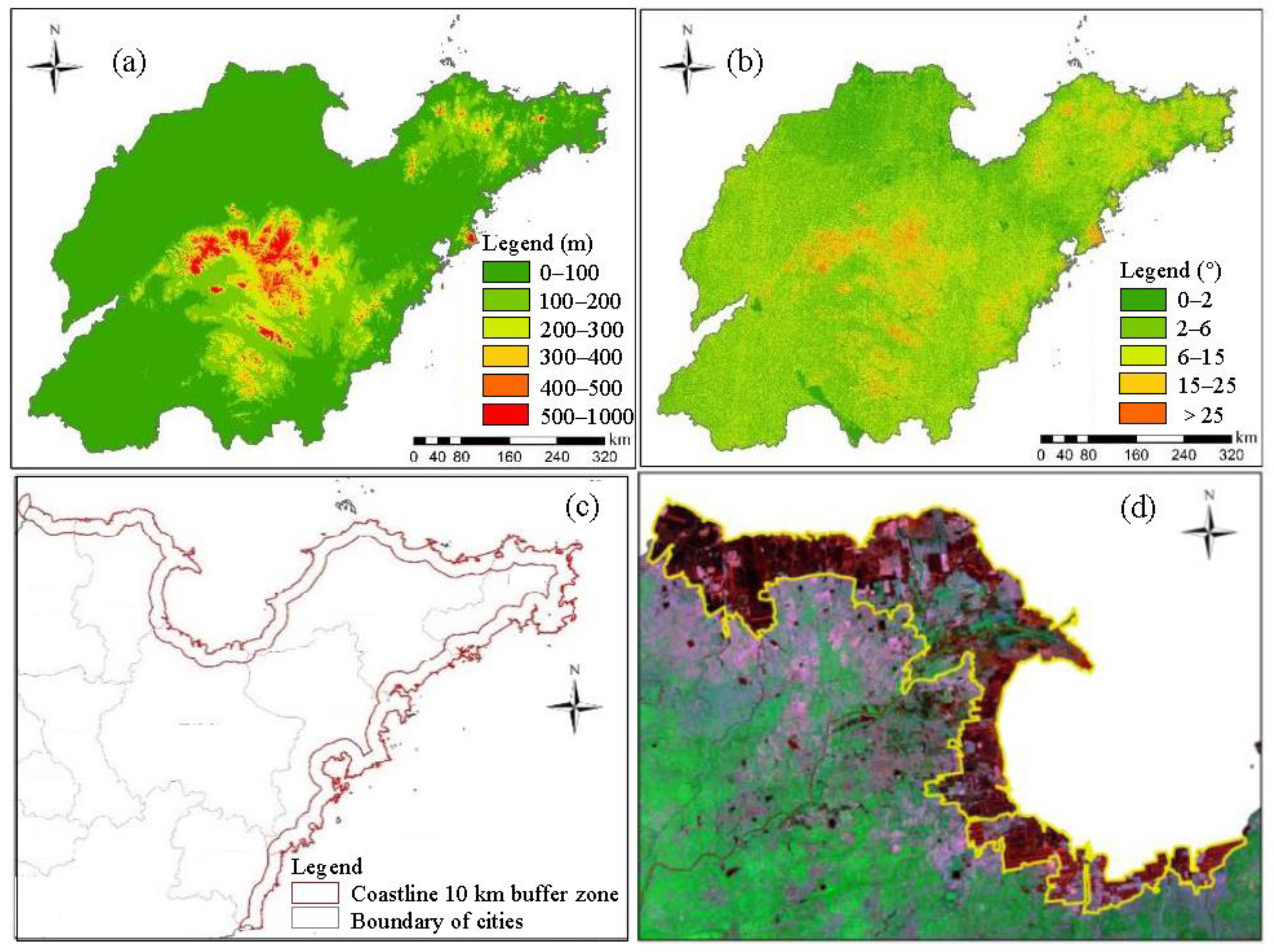
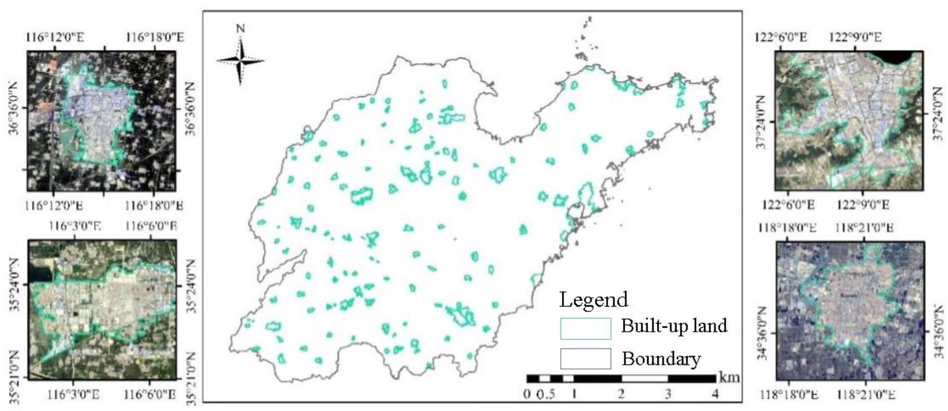
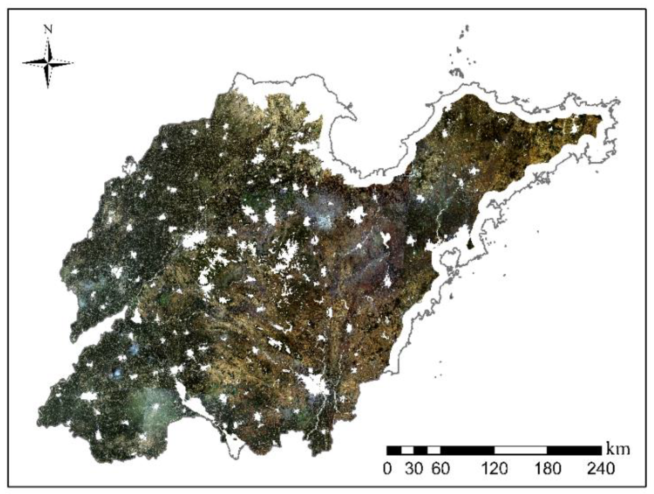
In terms of landform, in areas with an altitude of more than 500 m and a slope of more than 25°, the cropland is unstable, which can easily lead to a series of natural disasters, such as soil erosion, and threaten the safety of cropland. Therefore, China’s policy strictly prohibits the use of land with a slope greater than 25° for cropland, and such areas are generally not designated as PGs (Figure 2a,b). At the same time, the coastal zone near the Bohai Sea and the Yellow Sea has a high groundwater level, a cold ground temperature, difficulty rising, poor thermal insulation, and waterlogging. Combined with the actual situation, this study created a 10 km buffer zone for the coastline of the study area, which is regarded as an area where there are no PGs (Figure 2c). In terms of soil conditions, the greatest problem in the coastal zone is soil salinization. In these areas, the soil is sticky, the soil nutrient content is low, and the air permeability is poor. Most plants are endangered when the soil salt content is 0.3%, and they cannot grow when the soil salt content is greater than 0.5% (Figure 2d). In terms of land use types, non-agricultural construction land includes industrial and mining land, urban built-up land, rural residential land, transportation land, etc. Waterbodies include pits, ponds, water surfaces, lakes, rivers, ditches, and other water systems. These areas should be excluded during the identification of PGs (Figure 3, Figure 4 and Figure 5).

4.2. Optimal Segmentation Parameters of Plastic Greenhouse Segmentation

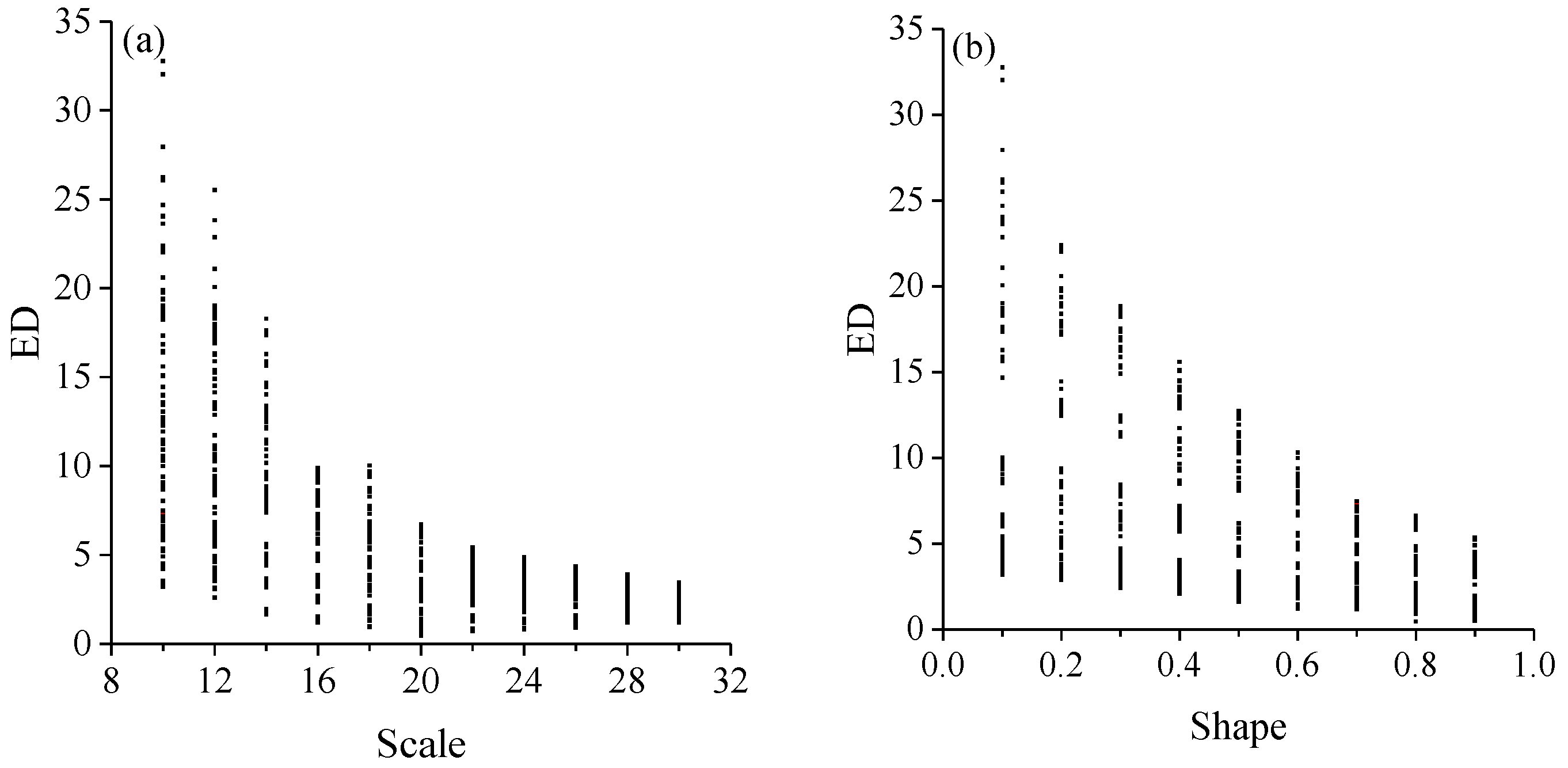
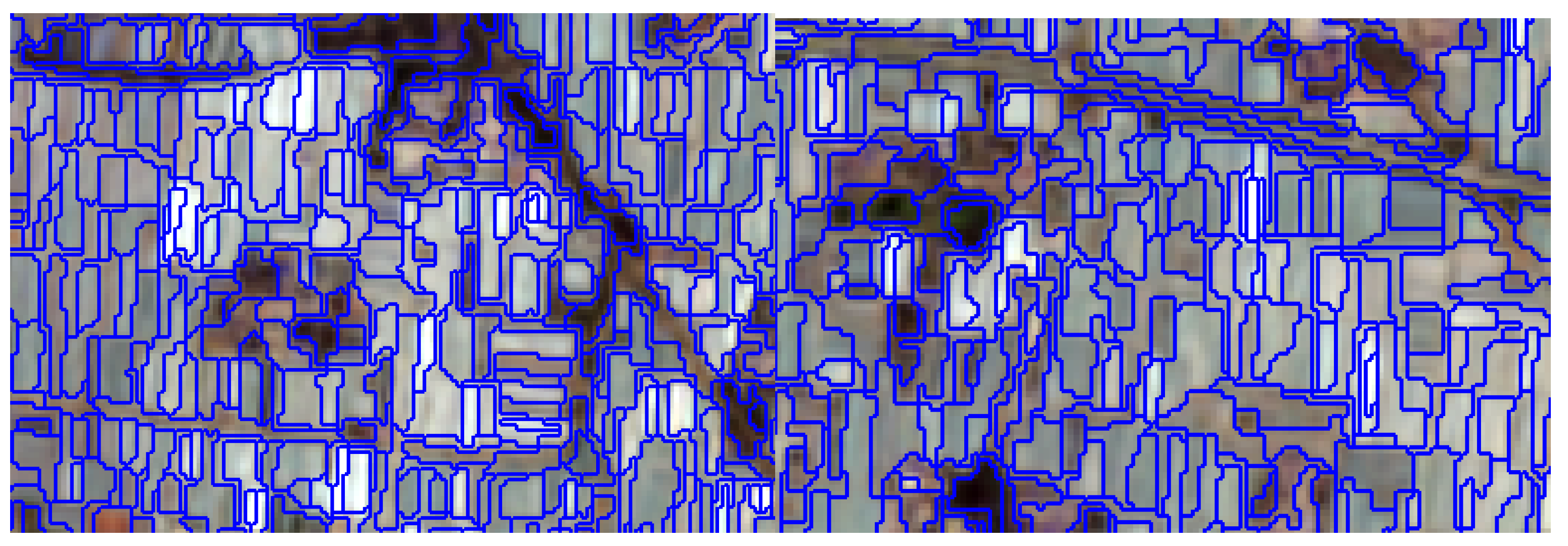
By analyzing the relationship between ED and the three segmentation parameters of scale, shape, and compactness, the best segmentation parameters can be determined. Figure 6a–c, respectively, show the change in ED caused by the changes in the other two parameters when the segmentation scale, shape, and compactness parameters are fixed at a certain value. With the increase in the segmentation scale value, the minimum value of the ED variation interval first gradually decreases and then increases. The scale parameter corresponding to the minimum value of ED is 20.0. The relationship between the ED and shape parameters is similar to that between the ED and scale parameters. When the shape parameter is 0.8, the minimum value of the ED variation interval reaches the lowest. ED has no significant relationship with the compactness parameter. The relationship between PSE and NSR presents an inverted triangle shape (Figure 6d). The point closest to the origin of the two-dimensional space meets the minimum PSE and NSR. At this time, the ED is the minimum, and the combination of segmentation parameters corresponding to this point is the optimal value. Therefore, in general, the optimal segmentation parameters of plastic greenhouse features in remote sensing images are scale = 20, shape = 0.8, and compactness = 0.5 (Figure 6). At this time, the minimum value of ED is 0.47 (Figure 7).

4.3. Study on the Optimal Characteristics of Plastic Greenhouse Space Variables by Remote Sensing

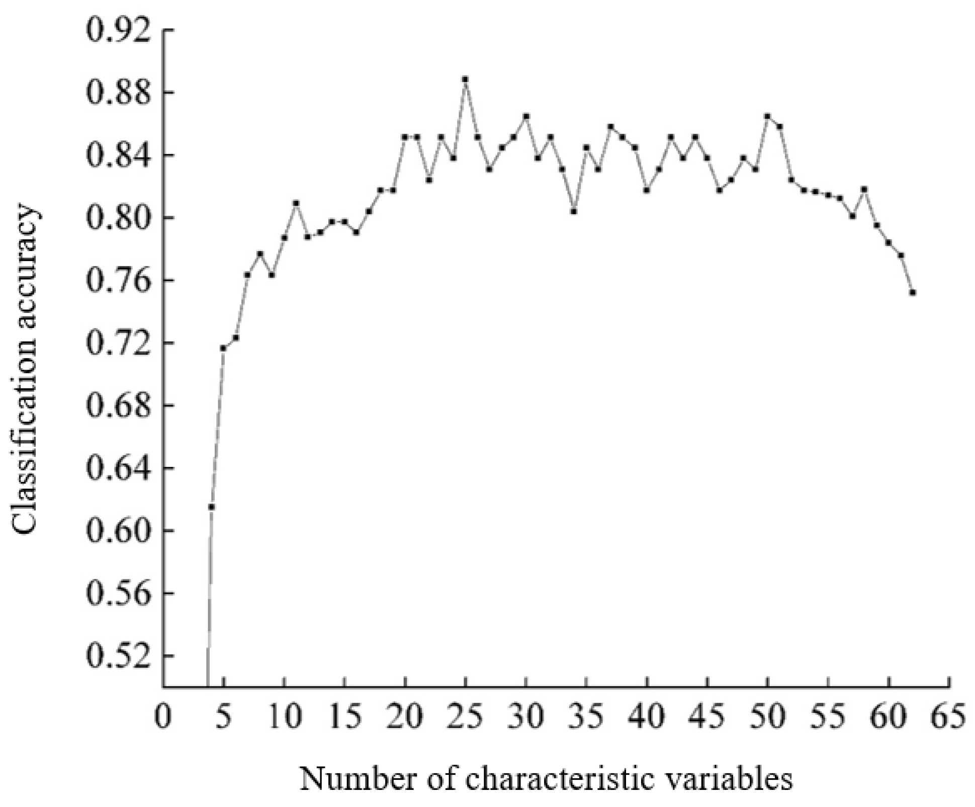
Based on the RDF, we score the importance of features, analyze the importance of 62 features to be selected, such as the spectrum, shape, and texture, and construct the optimal feature subset to improve the accuracy of the classification model. All the features to be selected are added to the RDF model, and the classification accuracy is only 0.75. With the sequential elimination of unimportant features in the feature set to be selected, the classification accuracy begins to show a gradual upward trend. After the addition of the remaining 52 features in the feature set to be selected, the classification accuracy fluctuates between 0.80 and 0.85. Among the 25 most important features, spectral, shape, and texture features play an important role, including the bands (Mean Layer 2, Mean Layer 5, and SWIR1_NIR, etc.) and the exponential features composed of bands (NDWI, GNDVI, SWIR2_NIR, NDVI, and PMLI), indicating that these features are important to distinguish PGs from other ground objects. In addition, texture features (contrast, variance) and the shape index (density and shape index) also play an important role (Figure 8 and Table 4).

4.4. Identification Accuracy of Three Different Classification Methods for PG in the Study Area

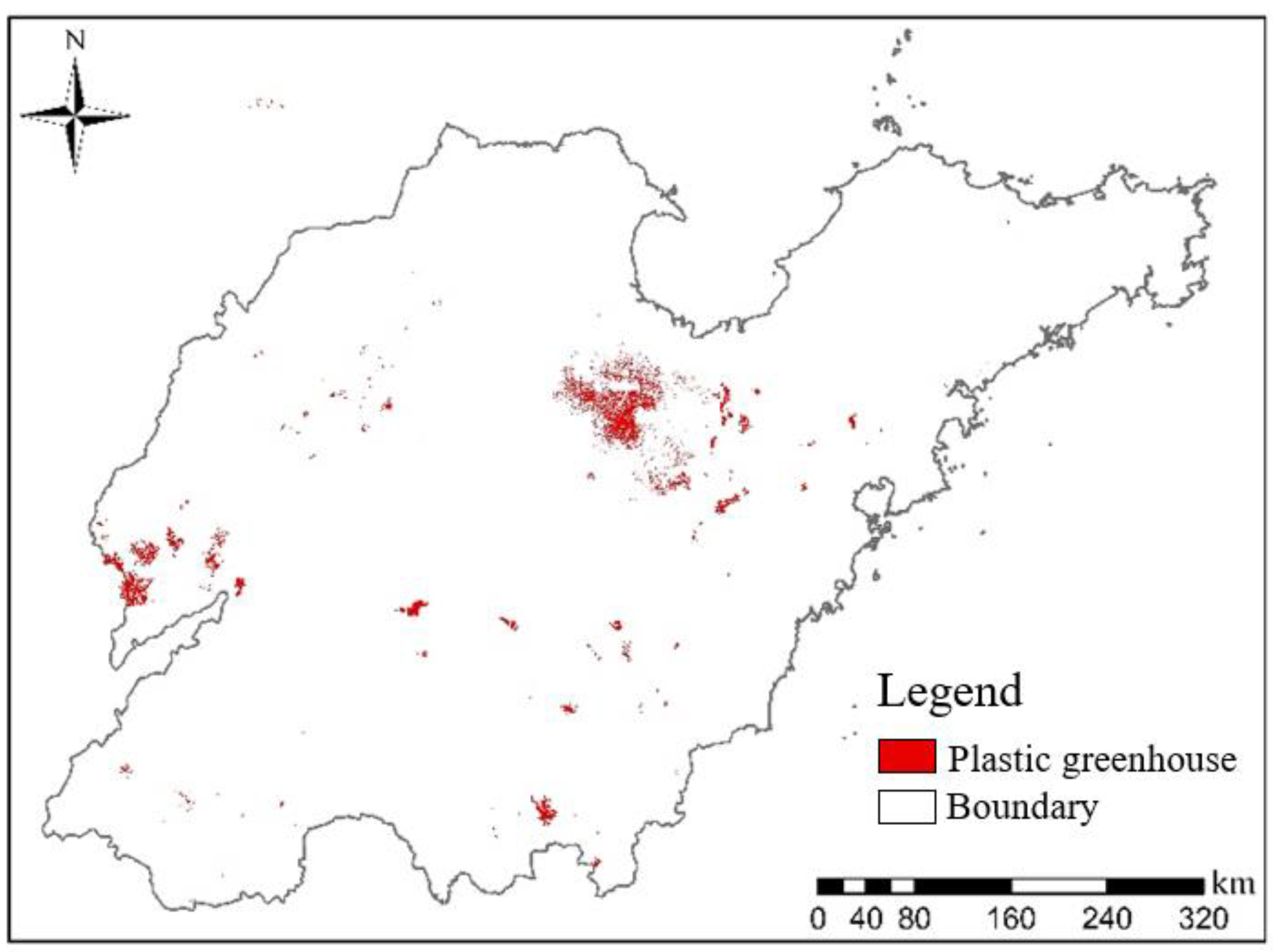
The overall evaluation accuracy of the SVM, CART, and RDF classifiers is calculated in order to select the most suitable classification model in PG recognition. The TP of the CART classification result is the smallest, the FN value is the largest, the R is 78.64%, the P is 82.70%, and the F value is 80.62%, indicating that this method is correctly classified, the area of PGs is the smallest, and the area of missed classification is the largest. This method has weak recognition ability for PGs, and it can easily classify PGs as other ground objects, with a low recall rate and low F value. The TP value, FN value, and FP value of the RDF are between those of the other two algorithms. The R is 84.06%, the P is 81.48%, and the F is 82.75%, indicating that the PG area correctly classified by this method is relatively large, and the areas of missed classification and misclassification are relatively small (Figure 9). Compared with the former two, the SVM has the largest TP value, the smallest FN value, and the largest FP value. The R is 93.25%, the P is 80.47%, and the F is close to 90%. It shows that the PGs with correct classification occupy the largest area and the smallest leakage area, so it is easy to classify other ground objects as PGs with this method. Generally speaking, based on the Landsat OLI image data, on the basis of contour recognition, CART, SVM, and RDF are used to extract the PGs, and the performance of SVM is the best (Figure 10 and Table 5).

5. Discussion

5.1. The Scope and Procedure of Unnecessary Spatial Operations Should Be Reduced by Combining Regional Features

In recent years, the deep learning model represented by neural networks has been widely used in the field of remote sensing [59]. Compared with traditional machine learning algorithms, such as SVM and RDF, deep learning needs massive samples to be model-driven, so there are many large-scale remote sensing image sample data sets. At the same time, these samples need the support of software and hardware equipment for big data storage and operation [60]. The most popular tools include the Orfeo Toolbox (OTB), the Remote Sensing and Geographic Information System Software Library (RGISLib), and the Scikit-learn Python libraries, which are commonly used for multispectral images acquired by drones with a higher spatial resolution [61,62,63]. With the development of remote sensing technology, a large number of satellite remote sensing data have emerged, such as high-resolution data with a spatial resolution less than the meter level (from Worldview, QuickBird, IKONOS, GF-2, and Planetscope, etc.) [64], hyperspectral or hyperspectral data with a spectral resolution of more than 100 bands (from EOS-AM1, EO-1, ARIES-1, and GF-5) [65], and data sets with a temporal resolution of less than one hour (from GOES-R, Meteosat, and FY series, etc.) [66]. Research institutions have also successively produced and released UC Merced, WHU-RS19, AID, and RSSCN7, providing data support for model structure optimization and algorithm strategy improvement [67]. In the process of identifying PGs, we used Landsat series data, which is a free data source with a lower spatial resolution than Sentinel-2 but a longer time span. Landsat was first launched in the 1970s, and Sentinel-2 was launched in June 2015. Therefore, the use of Landsat series data to study the mapping of PGs can help to understand the spatiotemporal dynamics and evolution of PGs over longer time series, so as to provide basic data for the management and decision making of relevant departments. Moreover, in the face of a large amount of data, the lack of systematic, comprehensive, and targeted remote sensing images and sample data sets can easily lead to problems. Thus, the ideal learning model and classifier should also be display familiarity with the topography, climate, meteorology, and ecological environment of the study area, and the efficiency of remote sensing recognition after expert screening will be improved [68].

5.2. The Corresponding Remote Sensing Data and Recognition Method Should Be Selected by Balancing Accuracy and Efficiency

PGs play an important role in the agricultural industry, so their development needs to be monitored and evaluated. However, in actual production and use, due to the differences in the thickness, density, transparency, color, and other materials covering the PG, as well as the differences in seasonal use and the types of plants planted in the greenhouse, it is difficult to extract the PGs by remote sensing [69]. In different remote sensing images, the features of the PGs are different from each other, such as their color, shape, texture, and spatial relationships [70]. Therefore, the methods and information used to extract the features of the PGs are different. At the same time, because of the different angles from which the sensor operates, the same type of land may have different spectral characteristics, leading to confusion with other non-plastic greenhouse land. At present, it is still a challenging task to use remote sensing to detect PGs. Moreover, the division factors and important features of different remote sensing data are different, and the efficiency is also different [71]. Lu et al. realized the spatiotemporal dynamics monitoring of large-area plastic greenhouses based on the spectral characteristics of Landsat 5TM images. However, the plastic film has high reflectivity and transparency to visible light, which leads to the complex spectral reflection characteristics of the PG, so it is difficult to accurately identify PGs with a single spectral feature [72]. Hasituya et al. and Aguera et al. found that when identifying PGs with medium- and low-resolution data, the overall precision of spectral features used alone was higher than that of texture features used alone [73,74]. None of these studies have taken into account the use of spatial elimination to first exclude regions where PGs cannot be present, and the recognition of PGs’ spectra, texture, and feature index is important. We suggest that the distribution characteristics of PGs should be fully considered, the regions where it is impossible to distribute PGs should be excluded first, and then the variables such as the spectrum, texture, and thematic index should be fully considered to identify PGs.

5.3. The Use of PGs Should Be Reduced and New Alternative Agricultural Facilities Sought

In 2010, the total area of PGs reached 365800 ha, mainly distributed in Asia, and China occupied 42.8% of the total area of the world. In order to meet the growing demand for vegetables, the PGs in China doubled in size from 2006 to 2010 [75]. More than 95% of the facilities were used to plant vegetables, and the total production amounted to more than trillions of tons [76]. It should be noted that plastic sheds are helpful for the production of farm products. However, the residual film affects and destroys the physical and chemical properties of the soil, resulting in difficulties in the growth and development of the roots of the plant, and it affects the normal absorption of water and nutrients by the roots [77]. At the same time, because of the limitations in the recovery of the residual film, and the incomplete treatment of the residual film, these films are often discarded on farmland and on the ground. After the wind blows, the residual film does not only affect the landscape environment, but also causes a long-term and extensive environmental problem because of its difficulty in degrading. Moreover, the plastic contains harmful substances such as alcohol and fluorine, which can affect the environment and are harmful for human health [78]. The spatial and temporal distribution information of plastic products is of great significance to the strategic planning of modern agriculture and the understanding of the impact of plastic products on the environment. Therefore, it is necessary to develop PG mapping methods that can automatically and accurately extract PG distribution information. The use of remote sensing images to observe the whole picture and frequency of large geographical areas has become a key technology to obtain surface information, providing the possibility for rapid large-scale geomorphic mapping.

6. Conclusions

In this study, Landsat OLI images were used as the data source, and the PG was the object of study. The best combination of the division factors and the construction of the best feature space in the image were studied. Then, the three methods of RDF, CART, and SVM were compared and analyzed, to extract the distribution area of the PGs in Shandong Province, in China.
(1) The method of object-oriented division could improve the accuracy of identification. The best division factors could be selected according to the three indexes, PSE, NSR, and ED. The best division factors for the specific object of the plastic greenhouse were scale = 20, shape = 0.8, and compactness = 0.5.
(2) The spectrum, texture, and shape of the remote sensing data were the key factors to identify the PGs. In the process of identifying the PGs, the features with more than 5% contributions included four band features, six band combination indexes, two shape features, i.e., density and the shape index, and two texture features, i.e., contrast and variance. These features played an important role in identifying the PGs.
(3) The three methods, CART, SVM, and RDF, were used to extract and compare the distribution areas of the PGs. It was found that the R values of CART, SVM, and RDF were 78.64%, 93.55%, and 84.06%. The P values of CART, SVM, and RDF were 82.70%, 80.47%, and 81.48%. Generally speaking, when the Landsat OLI remote sensing data were extracted from the PGs, the best effect was to combine the image division with SVM.
Our study focused only on a specific area, so it cannot be ruled out that the use of the same method in other areas will cause a decrease in accuracy. Although the extraction accuracy of our study was high, for a single random PG, due to the limited image resolution, its spectral and texture features are not clear, and there are omissions in classification and extraction. However, due to the limitations in segmentation, PGs separated by smaller distances are often classified as the same PG, resulting in an inaccurate PG count. These are areas that need to be improved in subsequent studies.

Author Contributions

Conceptualization, Y.Y. and M.S.; methodology, M.G.; software, Y.Y.; validation, M.S.; formal analysis, Y.Y.; investigation, M.G.; resources, M.S., M.G. and Y.Y.; data curation, M.G. and C.Z.; writing—original draft preparation, Y.Y.; writing—review and editing, M.S., L.X. and J.X.; visualization, L.X.; supervision, M.S.; project administration, M.S.; funding acquisition, Y.Y., M.S., C.Z. and G.Z. All authors have read and agreed to the published version of the manuscript.

Funding

This research was supported by the Youth Soft Science Research Project of Shanghai (23692120300), the Natural Science Foundation of Shanghai (23ZR1459700), the Yangfan Special Project of the Shanghai Qimingxing Program (22YF1444000), the National Key R&D Program of China (2017YFC0505504), and the Initiative Program for Young Scholars of Shanghai Academy of Landscape Architecture Science and Planning (KT00262, KT00258).

Data Availability Statement

Not applicable.

Conflicts of Interest

The authors declare that they have no known competing financial interest or personal relationships that could have appeared to influence the work reported in this paper.

Appendix A

Table A1. Land use types, landscape metrics, and other factors’ abbreviations.
TypeAbbreviationContent
Land use typesGLGrassland
CLCropland
SLShrubland
OLOrchard
BLBuilt-up land
WLWasteland
WBWaterbodies
FLForestland
Landscape metricsSVMSupport vector machine
CARTClassification and regression trees
RDFRandom decision forest
MPSMean patch area
CONTAGContagion index
SHIDShannon diversity index
COHESIONPatch cohesion Index
LSILandscape shape index
Socioeconomic factorsPOPPopulation
RURRural residents
URRUrban residents
GDPGross domestic product
PGDPPer capita gross domestic product
PRIPrimary sector
SECSecondary sector
TERTertiary sector
OthersMRYRRMiddle reaches of the Yangtze River region
Table A2. Characteristics of the above land types in Landsat OLI images.
TypeCategoryLandsat OLI ImageCharacteristic
CroplandCropland land with dense vegetationLand 12 02030 i001The vegetation coverage is high, the texture is smooth, and the general shape is regular.
Cropland land with sparse vegetationLand 12 02030 i002No vegetation, regular shape, contiguous distribution, smooth surface and dark brown.
VegetationGrasslandLand 12 02030 i003The surface is covered by vegetation, with a delicate texture and irregular shape, mostly distributed in the low mountains and hills of the study area.
ForestlandLand 12 02030 i004Vegetation coverage is high, dark green, generally distributed in patches, interlaced with grassland, granular surface.
Built-up landBuildings with blue roofsLand 12 02030 i005The roof is blue, rectangular in shape, concentrated in contiguous distribution, large scale.
Buildings with gray roofsLand 12 02030 i006The roofs are made of asphalt, mostly on the outskirts of the city, and appear grayish purple.
Buildings with red roofsLand 12 02030 i007The roof is red, generally concentrated, with a contiguous distribution in the suburbs or the central city.
RoadRoad that has been builtLand 12 02030 i008The shape of the road is slender and gray.
Road under constructionLand 12 02030 i009Due to the materials that need to be stored on the road in the construction process, the spectrum is not uniform, but mostly bright brown.
Mining land/Land 12 02030 i010No vegetation cover, the surface appears bright white, generally large area.
Bare land/Land 12 02030 i011Unvegetated, brown or bright brown, this category includes excavated land and bare ground, with a rough texture.
PGPG with thick plastic filmLand 12 02030 i012The surface covered with a sunshade net or grass curtain, dark purple or purple blue, regular shape and distribution.
PG with thin plastic filmLand 12 02030 i013Depending on the material, age, and type of crop grown, the plastic film appears in uneven bright white, green, or blue colors.
Table A3. The formula for calculating vegetation index with Landsat OLI images.
TypeFormula
NDVI(NIR − R)/(NIR + R)
NDWI(G − NIR)/(G + NIR)
Green NDVI (GNDVI)(NIR − G)/(NIR + G)
Plastic-mulched landover index (PMLI)(SWIR1 − NIR)/(SWIR1 + R)
SWIR1_NIR(SWIR1 − NIR)/(SWIR1 + NIR)
SWIR2_NIR(SWIR2 − NIR)/(SWIR2 + NIR)
Table A4. The formula for calculating texture features with Landsat OLI images.
Texture FeatureFormula
Energy i , j = 0 N 1 P i j ( i , j )
Correlation i , j = 0 N 1 P i j ( i u i ) ( i u j ) ( α i 2 ) ( α j 2 )
Dissimilarity i , j = 0 N 1 P i , j i j
Homogeneity i , j = 0 N 1 P i j 1 = ( i j ) 2
Contrast Y = i , j = 0 N 1 P i , j ( i j ) 2
Entropy i , j = 0 N 1 · P i , j ln P i , j
Mean i , j = 0 N 1 i · P i , j
Variance i , j = 0 N 1 i · P i , j i i , j = 0 N 1 i · P i , j
Note: N is the number of gray levels, P i , j is the entry (i,j) in the GLCM, u i and u j is the GLCM mean, α i 2 and α j 2 are the GLCM variance.

References

  1. Kalnay, E.; Cai, M. Impact of urbanization and land-use change on climate. Nature 2003, 423, 528. [Google Scholar] [CrossRef]
  2. Kabir, A.; Sekine, M.; Imai, T.; Yamamoto, K. Assessing Small-Scale Freshwater Microplastics Pollution, Land-use, Source-to-Sink Conduits, and Pollution Risks: Perspectives from Japanese Rivers Polluted with Microplastics. Sci. Total Environ. 2021, 768, 144655. [Google Scholar] [CrossRef] [PubMed]
  3. Shen, J.; Qin, G.; Yu, R.; Zhao, Y. Urbanization has changed the distribution pattern of zooplankton species diversity and the structure of functional groups. Ecoll. Indic. 2021, 120, 106944. [Google Scholar] [CrossRef]
  4. Tian, L.; Guo, Y. Peri-Urban China: Land Use, Growth, and Integrated Urban–Rural Development; Routledge: London, UK, 2019. [Google Scholar]
  5. Liu, D.; Zheng, X.; Wang, H. Land-use Simulation and Decision-Support system (LandSDS): Seamlessly integrating system dynamics, agent-based model, and cellular automata. Ecol. Model. 2020, 417, 108924. [Google Scholar] [CrossRef]
  6. Yi, Y.; Zhao, Y.; Ding, G.; Gao, G.; Shi, M.; Cao, Y. Effects of Urbanization on Landscape Patterns in a Mountainous Area: A Case Study in the Mentougou District, Beijing, China. Sustainability 2016, 8, 1190. [Google Scholar] [CrossRef]
  7. Zhu, Z.; He, Q.Y. Spatio-temporal Evaluation of the Urban Agglomeration Expansion in the Middle Reaches of the Yangtze River and Its Impact on Ecological Lands. Sci. Total Environ. 2021, 790, 148150. [Google Scholar]
  8. Dadashpoor, H.; Azizi, P.; Moghadasi, M. Land use change, urbanization, and change in landscape pattern in a metropolitan area. Sci. Total Environ. 2019, 655, 707–719. [Google Scholar] [CrossRef]
  9. National Bureau of Statistics of the People’s Republic of China. China Statistical Yearbook 2010; China Statistics Press: Beijing, China, 2011. [Google Scholar]
  10. National Bureau of Statistics of the People’s Republic of China. China Statistical Yearbook 2019; China Statistics Press: Beijing, China, 2020. [Google Scholar]
  11. Yang, Y. Spatiotemporal change characteristics of land landscape pattern in mountainous areas since reform and opening up: A case study of Mentougou District, Beijing. Subtrop. Soil Water Conserv. 2021, 33, 12–18. (In Chinese) [Google Scholar]
  12. Li, C.G.; Yin, H.F.; Chen, D.X.; Wang, B. Flood control problems and countermeasures in the middle reaches of the Yangtze River-Enlightenment from the devastating flood in 1998. Earth Sci. 1999, 4, 329–334. (In Chinese) [Google Scholar]
  13. Yi, Y.; Shi, M.; Liu, C.; Kang, H.; Wang, B. On landscape patterns in typical mountainous counties of middle reaches of the Yangtze River in China. Int. J. Environ. Res. Public Health 2021, 18, 4000. [Google Scholar] [CrossRef]
  14. Zheng, W.W. A Preliminary Study on Reasonable Forest Species Structure and Forest Coverage Rate in the Three Gorges Reservoir Area. Master’s Thesis, Beijing Forestry University, Beijing, China, 2006. (In Chinese). [Google Scholar]
  15. Arki, V.; Koskikala, J.; Fagerholm, N.; Kisanga, D.; K Käyhköa, N. Associations between local land use/land cover and place-based landscape service patterns in rural Tanzania. Ecosyst. Serv. 2020, 41, 101056. [Google Scholar] [CrossRef]
  16. Shehab, Z.N.; Jamil, N.R.; Aris, A.Z.; Shafie, N.S. Spatial variation impact of landscape patterns and land use on water quality across an urbanized watershed in Bentong. Malaysia. Ecol. Indic. 2021, 122, 107254. [Google Scholar] [CrossRef]
  17. Turner, B.L.; Skole, D.; Sanderson, S.; Fischer, G.; Fresco, L.; Leemans, R. Land Use and Land Cover Change: Science/Research Plan; IGBP Report No. 35 and HDP Report No. 7; IGBP: Stockholm, Sweden; Geneva, Switzerland, 1995; pp. 2–15. [Google Scholar]
  18. Castella, J.-C.; Kam, S.P.; Quang, D.D.; Verburg, P.H.; Hoanh, C.T. Combining top-down and bottom-up modelling approaches of land use/cover change to support public policies: Application to sustainable management of natural resources in northern Vietnam. Land Use Policy 2007, 24, 531–545. [Google Scholar] [CrossRef]
  19. Verburg, P.H.; Schot, P.P.; Dijst, M.J.; Veldkamp, A. Land use change modelling: Current practice and research priorities. Geojournal 2004, 61, 309–324. [Google Scholar] [CrossRef]
  20. Spencer, R.; Meyer, K.B.; Christopher, S.C.; Robert, J.L. An analysis of spatio-temporal landscape patterns for protected areas in northern New England: 1900–2010. Landsc. Ecol. 2015, 30, 1291–1305. [Google Scholar]
  21. Zhou, Y.Y.; Yue, D.X.; Guo, J.J.; Chen, G.G.; Wang, D. Spatial correlations between landscape patterns and net primary productivity: A case study of the Shule River Basin, China. Ecol. Indic. 2021, 130, 94–104. [Google Scholar] [CrossRef]
  22. Forman, R.T.T.; Godron, M. Landscape Ecology; John Wiley & Sons: New York, NY, USA, 1986. [Google Scholar]
  23. Pickett, S.T.A.; Cadenasso, M.L. Landscape ecology: Spatial heterogeneity in ecological systems. Science 1995, 269, 331–334. [Google Scholar] [CrossRef]
  24. Turner, M.G.; Gardner, R.H. Quantitative Methods in Landscape Ecology; Springer: New York, NY, USA, 1991. [Google Scholar]
  25. Risser, P.G.; Iverson, L.R. 30 years later—Landscape ecology: Directions and approaches. Landsc. Ecol. 2013, 28, 367–369. [Google Scholar] [CrossRef]
  26. Wang, X.L.; Xiao, D.N. Landscape pattern analysis of liaohe Delta wetland. Acta Ecol. Sin. 1997, 17, 317–323. (In Chinese) [Google Scholar]
  27. Wu, J.; Levin, S.A. A spatial patch dynamic modeling approach to pattern and process in an annual grassland. Ecol. Monogr. 1994, 64, 447–464. [Google Scholar] [CrossRef]
  28. Zhang, M.; Tan, S.; Zhang, C.; Han, S.; Zou, S.; Chen, E. Assessing the impact of fractional vegetation cover on urban thermal environment: A case study of Hangzhou, China. Sustain. Cities Soc. 2023, 96, 104663. [Google Scholar] [CrossRef]
  29. Liu, Z.; Liu, W.; Walker, T.; Adams, M.; Zhao, J. How does the global plastic waste trade contribute to environmental benefits: Implication for reductions of greenhouse gas emissions? J. Environ. Manag. 2021, 287, 112283. [Google Scholar] [CrossRef] [PubMed]
  30. Hasituya; Chen, Z.; Li, F.; Hu, Y. Mapping plastic-mulched farmland by coupling optical and synthetic aperture radar remote sensing. Int. J. Remote Sens. 2020, 41, 7757–7778. [Google Scholar] [CrossRef]
  31. Yi, Y.; Shi, M.; Wu, J.; Yang, N.; Zhang, C.; Yi, X. Spatio-Temporal Patterns and Driving Forces of Desertification in Otindag Sandy Land, Inner Mongolia, China, in Recent 30 Years. Remote Sens. 2023, 15, 279. [Google Scholar] [CrossRef]
  32. Chen, W.; Xu, Y.M.; Zhang, Z.; Yang, L.; Pan, X.B.; Jia, Z. Mapping agricultural plastic greenhouses using Google Earth images and deep learning. Comput. Electron. Ariculture 2021, 191, 106552. [Google Scholar] [CrossRef]
  33. Antrop, M. Landscape change and the urbanization process in Europe. Landsc. Urban Plan. 2004, 67, 9–26. [Google Scholar] [CrossRef]
  34. Wu, J.G.; Jenerette, G.D.; Buyantuyev, A.; Redman, C.L. Quantifying spatiotemporal patterns of urbanization: The case of the two fastest growing metropolitan regions in the United States. Ecol. Complex. 2011, 8, 1–8. [Google Scholar] [CrossRef]
  35. Zhu, C.M.; Zhang, X.L.; Zhou, M.M.; He, S.; Gan, M.Y.; Yang, L.X.; Wang, K. Impacts of urbanization and landscape pattern on habitat quality using OLS and GWR models in Hangzhou, China. Ecol. Indic. 2020, 117, 106654. [Google Scholar] [CrossRef]
  36. Zhang, P.; Du, P.; Guo, S.; Zhang, W.; Tang, P.; Chen, J.; Zheng, H. A novel index for robust and large-scale mapping of plastic greenhouse from Sentinel-2 images. Remote Sens. Environ. 2022, 276, 113042. [Google Scholar] [CrossRef]
  37. Du, X.; Huang, Z. Ecological and environmental effects of land use change in rapid urbanization: The case of hangzhou, China. Ecol. Indicator. 2017, 81, 243–251. [Google Scholar] [CrossRef]
  38. Novelli, A.; Aguilar, M.; Nemmaoui, A.; Aguilar, F.; Tarantino, E. Performance evaluation of object based greenhouse detection from Sentinel-2 MSI and Landsat 8 OLI data: A case study from Almería (Spain). Int. J. Appl. Earth Obs. Geoinf. 2016, 52, 403–411. [Google Scholar] [CrossRef]
  39. Yuan, Z.; Xu, J.; Wang, Y.; Yan, B. Analyzing the influence of land use/land cover change on landscape pattern and ecosystem services in the Poyang Lake Region, China. Environ. Sci. Pollut. Res. 2021, 28, 27193–27206. [Google Scholar] [CrossRef]
  40. Mark, M.; Fu, B. Evaluation of landscape pattern and fragmentation in Dongling Mountain area, Beijing. Chin. J. Plant Ecol. 2000, 1, 320–326. (In Chinese) [Google Scholar]
  41. Guo, X.; Li, P. Mapping plastic materials in an urban area: Development of the normalized difference plastic index using WorldView-3 superspectral data. ISPRS J. Photogramm. Remote Sens. 2020, 169, 214–226. [Google Scholar] [CrossRef]
  42. Arcidiacono, C.; Porto, S.M.C. Classification of crop-shelter coverage by RGB aerial images: A compendium of experiences and findings. J. Agric. Eng. 2010, 41, 1. [Google Scholar] [CrossRef]
  43. Sobbahi, R.; Tekli, J. Comparing deep learning models for low-light natural scene image enhancement and their impact on object detection and classification: Overview, empirical evaluation, and challenges. Signal Process. Image Commun. 2022, 109, 116848. [Google Scholar] [CrossRef]
  44. Kim, J.H.; Kwon, O.S.; Ra, J.H. Urban Type Classification and Characteristic Analysis through Time-Series Environmental Changes for Land Use Management for 31 Satellite Cities around Seoul, South Korea. Land 2021, 10, 799. [Google Scholar] [CrossRef]
  45. Huang, C.; Huang, X.; Peng, C.; Zhou, Z.; Teng, M.; Wang, P. Land use/cover change in the Three Gorges Reservoir area, China: Reconciling the land use conflicts between development and protection. Catena 2019, 175, 388–399. [Google Scholar] [CrossRef]
  46. Asimeh, M.; Nooripoor, M.; Azadi, H.; Hossein, A.; Veerle, V.E.; Petr, S.; Frank, W. Agricultural land use sustainability in Southwest Iran: Improving land leveling using consolidation plans. Land Use Policy 2020, 94, 104555. [Google Scholar] [CrossRef]
  47. Li, H.; Peng, J.; Liu, Y.; Hu, Y. Urbanization impact on landscape patterns in Beijing City, China: A spatial heterogeneity perspective. Ecol. Ind. 2017, 82, 50–60. [Google Scholar] [CrossRef]
  48. Yi, Y.; Wang, B.; Shi, M.; Meng, Z.; Zhang, C. Variation in Vegetation and Its Driving Force in the Middle Reaches of the Yangtze River in China. Water 2021, 13, 2036. [Google Scholar] [CrossRef]
  49. Ng, C.N.; Xie, Y.J.; Yu, X.J. Measuring the spatio-temporal variation of habitat isolation due to rapid urbanization: A case study of the Shenzhen River cross-boundary catchment, China. Landsc. Urban Plan. 2011, 103, 44–54. [Google Scholar] [CrossRef]
  50. Long, H.L.; Heilig, G.K.; Wang, J.; Li, X.B.; Luo, M.; Wu, X.Q.; Zhang, M. Land use and soil erosion in the upper reaches of the Yangtze River: Some socio-economic considerations on China’s Grain-for-Green Programme. Land Degrad. Dev. 2006, 17, 589–603. [Google Scholar] [CrossRef]
  51. Yang, D.; Chen, J.; Zhou, Y.; Chen, X.; Chen, X.; Cao, X. Mapping plastic greenhouse with medium spatial resolution satellite data: Development of a new spectral index. ISPRS J. Photogramm. Remote Sens. 2017, 128, 47–60. [Google Scholar] [CrossRef]
  52. Yi, Y.; Shen, G.; Zhang, C.; Sun, H.; Zhang, Z.; Yin, S. Quantitative analysis and prediction of urban heat island intensity on urban-rural gradient: A case study of Shanghai. Sci. Total Environ. 2022, 22, 154264. [Google Scholar] [CrossRef]
  53. Li, M.; Zhang, Z.; Lei, L.; Wang, X.; Guo, X. Agricultural Greenhouses Detection in High-Resolution Satellite Images Based on Convolutional Neural Networks: Comparison of Faster R-CNN, YOLO v3 and SSD. Sensors 2020, 20, 4938. [Google Scholar] [CrossRef]
  54. Li, Y.; Wang, J.; Yang, S.; Zhang, S. Occurrence, health risks and soil-air exchange of phthalate acid esters: A case study in plastic film greenhouses of Chongqing. China. Chemosphere 2021, 268, 128821. [Google Scholar] [CrossRef]
  55. Wu, C.; Deng, J.; Wang, K.; Ma, L.; Tahmassebi, A.R.S. Object-based classification approach for greenhouse mapping using Landsat-8 imagery. Int. J. Agric. Biol. Eng. 2016, 9, 79–88. [Google Scholar]
  56. Gonzalez-Yebra, O.; Aguilar, M.A.; Nemmaoui, A.; Aguilar, F.J.; Urbano, D.S. Methodological proposal to assess plastic greenhouses land cover change from the combination of archival aerial orthoimages and Landsat data. Biosyst. Eng. 2018, 175, 36–51. [Google Scholar] [CrossRef]
  57. Parlato, M.; Valenti, F.; Porto, S. Covering plastic films in greenhouses system: A GIS-based model to improve post use suistainable management. J. Environ. Manag. 2020, 2363, 110389. [Google Scholar] [CrossRef]
  58. Nguyen, H.; Pan, V.; Pham, C.; Valdez, R.; Doan, K.; Nansen, C. Night-based hyperspectral imaging to study association of horticultural crop leaf reflectance and nutrient status. Comput. Electron. Agric. 2020, 173, 105458. [Google Scholar] [CrossRef]
  59. Gonzalez-Avila, S.; Lopez-Leiva, C.; Bunce, R.G.H.; Elena-Rosselló, R. Changes and drivers in Spanish landscapes at the Rural-Urban Interface between 1956 and 2018. Sci. Total Environ. 2020, 714, 136858. [Google Scholar] [CrossRef]
  60. Liu, R.; Zhu, D. Discussion on land use change information mining method based on transition matrix. Resour. Sci. 2010, 32, 1544–1550. [Google Scholar]
  61. Stupariu, M.; Cushman, S.; Pleşoianu, A.; Pătru-Stupariu, L.; Fürst, C. Machine learning in landscape ecological analysis: A review of recent approaches. Landsc. Ecol. 2021, 37, 1227–1250. [Google Scholar] [CrossRef]
  62. Lourenço, P.; Teodoro, A.; Gonçalves, J.; Honrado, J.; Cunha, M.; Sillero, N. Assessing the performance of different OBIA software approaches for mapping invasive alien plants along roads with remote sensing data. Int. J. Appl. Earth Obs. Geoinf. 2021, 95, 102263. [Google Scholar] [CrossRef]
  63. Sikakwe, G. Mineral exploration employing drones, contemporary geological satellite remote sensing and geographical information system (GIS) procedures: A review. Remote Sens. Appl. Soc. Environ. 2023, 31, 100988. [Google Scholar] [CrossRef]
  64. Aguilera-Martos, I.; García-Vico, A.; Luengo, J.; Damas, S.; Melero, F.; Valle-Alonso, J.; Herrera, F. TSFEDL: A python library for time series spatio-temporal feature extraction and prediction using deep learning. Neurocomputing 2023, 517, 223–228. [Google Scholar] [CrossRef]
  65. Haq, M. Planetscope Nanosatellites Image Classification Using Machine Learning. Comput. Syst. Sci. Eng. 2022, 3, 1031–1046. [Google Scholar] [CrossRef]
  66. Xiao, R.; Wang, G.; Zhang, Q.; Zhang, Z. Multi-scale analysis of relationship between landscape pattern and urban river water quality in different seasons. Sci. Rep. 2016, 6, 25250. [Google Scholar] [CrossRef] [PubMed]
  67. Hope, A.S.; Boynton, W.L.; Stow, D.A.; Douglas, D.C. Interannual growth dynamics of vegetation in the Kuparuk River watershed, Alaska based on the Normalized Difference Vegetation Index. Int. J. Remote Sens. 2003, 24, 3413–3425. [Google Scholar] [CrossRef]
  68. Zhou, D.; Xu, J.C.; Wang, L.; Lin, Z.L. Assessing urbanization quality using structure and function analyses: A case study of the urban agglomeration around Hangzhou Bay (UAHB), China. Habitat Int. 2015, 49, 165–176. [Google Scholar] [CrossRef]
  69. Zhang, C.; Zhang, M.M. Wavelet-based neural network with genetic algorithm optimization for generation prediction of PV plants. Energy Rep. 2022, 8, 10976–10990. [Google Scholar] [CrossRef]
  70. Xu, N. Study on the Spatial Pattern of Land Use in the Yangtze River Delta from 2000 to 2010; Xi’an University of Science and Technology: Xi’an, China, 2014. [Google Scholar]
  71. Ye, C.S.; Wang, F. Study on land use and landscape pattern change in Pearl River Delta. Bull. Soil Water Conserv. 2012, 32, 238–243. [Google Scholar]
  72. He, Y.; Wang, J.J.; Yuan, Z.J.; Zheng, M.G.; Huang, B.; Liang, C. Land use change and its response to urbanization in the Pearl River Delta. Ecol. Environ. Sci. 2020, 29, 303–310. [Google Scholar]
  73. Lu, L.; Di, L.; Ye, Y. A decision-tree classifier for extracting transparent plastic-mulched landcover from landsat-5 TM images. IEEE J. Sel. Top. Appl. Earth Obs. Remote Sens. 2014, 7, 4548–4558. [Google Scholar] [CrossRef]
  74. Hasituya; Chen, Z.; Wang, L.; Wu, W.; Jiang, Z.; Li, H. Monitoring Plastic-mulched farmland by landsat8 OLI imagery using spectral and textural features. Remote Sens. 2016, 8, 353. [Google Scholar] [CrossRef]
  75. Agüera, F.; Aguilar, F.J.; Aguilar, M.A. Using texture analysis to improve per-pixel classification of very high resolution images for mapping plastic greenhouses. ISPRS J. Photogramm. Remote Sens. 2008, 63, 635–646. [Google Scholar] [CrossRef]
  76. Zhu, B.; Zhang, T.L. The impact of cross-region industrial structure optimization on economy, carbon emissions and energy consumption: A case of the Yangtze River Delta. Sci. Total Environ. 2021, 778, 146089. [Google Scholar] [CrossRef]
  77. Yu, Z.; Li, X.F.; Wang, S.R.; Liu, L.Y.; Zeng, E.Y. The human and ecological risks of neonicotinoid insecticides in soils of an agricultural zone within the Pearl River Delta, South China. Environ. Pollut. 2021, 284, 117358. [Google Scholar] [CrossRef]
  78. Zhao, Y.; Liu, Y.Z.; Long, K.S. Characteristics and influencing factors of urban land development intensity in Yangtze River Delta. Resour. Environ. Yangtze Basin 2012, 21, 1480–1485. [Google Scholar]
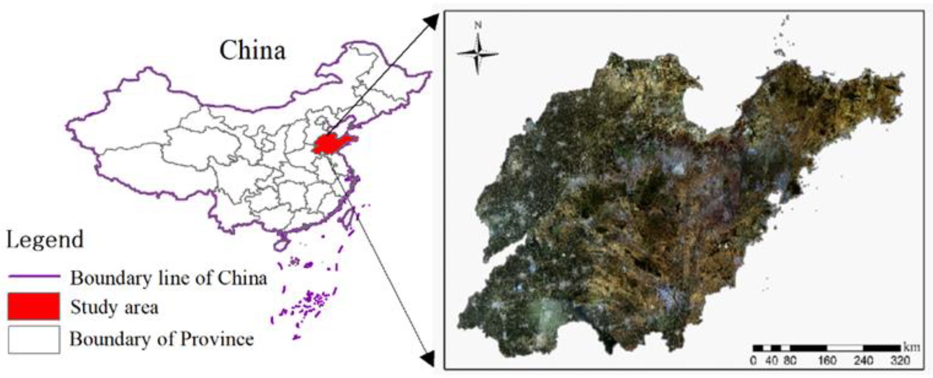
Figure 1. Locations of the study areas.
Land 12 02030 g001
Figure 2. Spatial analysis of geographical environment data in the study area: (a) elevation; (b) aspect; (c) coastline; and (d) salinized soil.
Land 12 02030 g002
Figure 3. Spatial distribution of waterbodies in the study area.
Land 12 02030 g003
Figure 4. Spatial distribution of built-up land in the study area.
Land 12 02030 g004
Figure 5. The spatial range in which PGs may be distributed in the study area.
Land 12 02030 g005
Figure 6. The scattergrams of the segmentation parameter. (a) Relationship between ED and scale parameters; (b) relationship between ED and shape parameters; (c) relationship between ED and compactness parameters; (d) relationship between PSE and NSR. Note: Each dot indicates a combination of parameter values.
Land 12 02030 g006aLand 12 02030 g006b
Figure 7. The segmentation result of the optimal segmentation parameters of PG.
Land 12 02030 g007
Figure 8. The relationship between the number of features and the accuracy of classification.
Land 12 02030 g008
Figure 9. Comparison of extraction of PG results between different methods and artificial interpretation. (a) Comparison by SVM and real sample distributions; (b) Comparison by CART decision tree and real sample distributions; (c) Comparison by RDF and real sample distributions.
Land 12 02030 g009
Figure 10. The PG distribution area of the study area.
Land 12 02030 g010
Table 1. OIF index in descending order for each band combination of Landsat OLI images.
Types123456
Combined bands456457256257357356
OIF1375.491375.091313.581305.591290.251277.99
Table 2. List of features to be selected for the classifier.
Band FeaturesBand Combination FeaturesShape FeaturesTexture Features
Mean Layer i (i = 1, 2…7)NDVIAreaEnergy
Ratio Layer i (i = 1, 2…7)NDWILengthCorrelation
Standard Deviation Layer i (i = 1, 2…7)GNDVIWidthDissimilarity
Mean Diff. from Neighboring Layer i (i = 1, 2…7)PMLILength/widthHomogeneity
Contrast to Neighboring Pixels i (i = 1, 2…7)SWIR1_NIRDensityContrast
BrightnessSWIR2_NIRCompactnessEntropy
Maximum Difference Score Rectangular fitMean
Main directionVariance
Roundness
Border index
Shape index
Table 3. List of accuracy evaluation indexes for classifier.
IndicatorFormulaContent
TP/The area of PGs correctly classified
FP/The area classified as greenhouse plastic is actually the area of other features
FN/The area that is actually PG but is classified as other features
RTP/(TP + FN)The proportion of correctly classified plastic greenhouses to the total area of the reference data set
PTP/(TP + FP)The proportion of correctly classified PGs to total classified area
F2 × P × R/(P + R)The mean value of recall and precision
Note: TP represents true positives; FP represents false positives; FN represents false negatives; R represents recall; P represents precision; and F represents the F-measure.
Table 4. The optimal feature subset and importance sorting.
OrderTypesVariableContribution
1BandMean Layer 28.24
2BandMean Layer 58.23
3TextureContrast7.56
4Band combinationSWIR2_NIR7.37
5ShapeDensity7.14
6Band combinationNDWI7.09
7Band combinationGNDVI6.62
8TextureVariance6.37
9Band combinationSWIR1_NIR6.24
10BandContrast to neighboring pixels 56.03
11Band combinationNDVI6.00
12Band combinationPMLI5.59
13ShapeShape index5.35
14BandMean diff. from neighboring layer 65.18
15 Others≤5.00
Table 5. Results of accuracy evaluation for three methods in extraction of PGs.
Classification MethodTP (km2)FN (km2)FP (km2)R (%)P (%)F (%)
SVM57.0941.3213.8593.2580.4786.39
CART48.1413.0810.0778.6482.7080.62
RDF51.4697.5811.7084.0681.4882.75
Note: SVM represents support vector machine; CART represents classification and regression trees; RDF represents random decision forest.
Disclaimer/Publisher’s Note: The statements, opinions and data contained in all publications are solely those of the individual author(s) and contributor(s) and not of MDPI and/or the editor(s). MDPI and/or the editor(s) disclaim responsibility for any injury to people or property resulting from any ideas, methods, instructions or products referred to in the content.