Abstract
Flood risk assessment at the mesoscale requires data that are spatially and thematically detailed enough to provide reliable estimates at the catchment level. However, data availability and suitability are often contradictory: available data are rarely suitable at the required level of detail. To overcome this problem, numerous disaggregation methods have been proposed in recent decades, often based on somewhat generalised imperviousness characteristics derived from the available urban land use/land cover (LULC) nomenclature. To reduce generalisation, we propose a new disaggregation approach using a spatially distributed imperviousness density (IMD) layer at a very detailed spatial resolution of 10 m as ancillary data to improve the thematic detail of the urban classes of the available LULC datasets (Coastal Zones, Natura 2000) and the dasymetric mapping of the census data. The nomenclature of the urban classes and the impervious density thresholds were taken from the detailed Urban Atlas dataset. The disaggregation of the census data is then built on the resulting geometry of thematically improved residential classes. Assuming that IMD values indicate a built-up density, the proposed weighting scheme is IMD-dependent: it accounts for variability in the built-up density and, hence, variability in population. The approach was tested in three catchments in Croatia, each with a different degree of urbanisation. The resulting statistics (mean square error and percentage error) indicate that residential areas and population density depend on IMD. Using IMD as additional data therefore greatly improves the assessment of elements that are exposed to flooding and, consequently, the damage and flood risk assessment.
1. Introduction
Floods affect billions of people, more than any other environmental hazard. Recent global estimates indicate that 23% of the world’s population is directly exposed to 100-year floods [1]. These estimates are expected to increase by 2030, especially in countries with high rates of urbanisation [2,3,4]. Flood damage causes human suffering and major economic losses in the form of damaged properties and infrastructure. In 2021 alone, 223 floods occurred (compared to 163 for the 2001–2020 annual average), causing 29.2 million deaths and USD 74.4 billion of economic damage [5]. Based on the CATDAT database records, 43% of the total economic losses caused by natural hazards in EU countries between 1980 and 2020 are due to unfavourable hydrological events [6]. The increasing trend in flood damages over past decades has made flood management even more challenging, requiring a paradigm shift from traditional flood control to more effective flood risk management [7]. The need for a change in flood policy has led to the adoption of the EU Floods Directive (2007/60/EC, 2007), which focuses on reducing risks rather than preventing flooding through structural measures (grey infrastructure).
Flood risk management requires a complex analysis carried out in several stages (e.g., [8,9,10,11]). In general, the process starts with the derivation of the probability and intensity of flood events and the preparation of flood hazard maps. To locate assets and populations that are exposed to flooding, socio-economic data are overlaid with flood characteristics, and finally, exposure information is related to monetary values, leading to the estimation of flood damages and the production of flood risk maps. The estimation of damage caused by floods is a necessary step in flood risk management. It provides relevant information for the calculation of post-flood compensation (essential information for flood insurance) and supports decision making regarding risk reduction measures [7,12,13]. The estimated damages usually refer to direct, tangible damages that can be quantified using depth–damage curves by relating the water depth to the damages to vulnerable elements (assets exposed to flooding).
The level of detail of the mapping of elements at risk depends primarily on the spatial extent of the flood-prone area and the level of detail of the damage assessment. As pointed out by Messner and Meyer [14], flood damage assessment is usually carried out on three main scales in relation to the extent of the area at risk and, consequently, the spatial and thematic level of detail of the data: the macro, meso and micro scales, while de Moel at al [8] also discuss the fourth supranational scale. The main distinguishing feature between the scales is the level of spatial and thematic aggregation. The supranational level refers to the continental-to-global scale and requires a low spatial resolution (1–10 km). At the macro level, damage assessment is carried out at the level of large spatial units such as countries or municipalities, while at the meso level, more detail is required, resulting from spatial aggregation [7], e.g., residential areas or urban green spaces. The spatial resolution required for flood risk assessment at the macro and meso levels varies between 100–1000 m and 25–100 m, respectively. The most detailed microscale (local) level requires very detailed spatial (1–25 m) and thematic data, i.e., land use/land cover (LULC) at the object level, albeit with some degree of thematic generalisation: similar objects are grouped into classes where all elements are assumed to share the same characteristics (e.g., residential homes, indoor sports facilities).
At all spatial scales, flood risk assessment is subject to many uncertainties that affect performance to a greater or lesser extent. These uncertainties may be related to the behaviour of the observed system (spatially and temporally) and the acquired knowledge about the system, including insufficient quality and/or quantity of data in relation to the scale of investigation. Sources of uncertainty are present at all stages of the assessment, i.e., flood hazard mapping, exposure analysis of the elements at risk, estimation of the value and susceptibility analysis of the elements at risk [15,16,17].
Flood hazard and flood risk mapping requires large amounts of input data, including meteorological and hydrological data, as well as various spatial data such as detailed topographic features and LULC data. Insufficient input data, especially spatial data describing topography or assets and people affected by flooding, is often the main source of uncertainty in flood risk. This can be caused by the lack of correspondence between the level of detail of the spatial data and the scale of investigation, but also by the level of detail within the different stages of flood risk assessment (flood hazard maps are the result of a 2D hydrodynamic model based on spatially detailed raster data [18,19,20,21,22], while the relationship between the extent of damage and the flood depth is available for the specific LULC categories in the form of depth–damage curves (e.g., [23,24,25,26,27]).
At the macro and meso levels of study, the data needed for the assessment contain different levels of aggregation. Often, population and LULC data are not spatially and thematically detailed enough to meet the needs at the meso level. They are collected at an aggregated level, e.g., at the level of census units (usually settlements or municipalities) and LULC categories associated with a particular economic sector [28]. The determination of the potential economic damage caused by a flood is a critical point in the assessment of flood risk [11] and is based on the assignment of the corresponding depth–damage curve to the existing land use category. The curves describe the flood damage that would occur for a given water depth per asset or per land use category. The global depth–damage functions issued by the European Commission [29] were developed for six major land use classes: residential, commercial, industrial, transport, infrastructure—roads and agricultural (Figure 1).
Figure 1.
Depth–damage curves for different land use categories [29].
The acquisition of high-resolution data requires a great amount of funds and effort. On the other hand, with Earth observation systems providing continuous and synoptic surface observations as well as freely available medium- and low-resolution data, LULC datasets have become widely available, although they are primarily suitable for continental- and national-scale investigations. The GlobeLand30 dataset, for example, provides detailed LULC data with a spatial resolution of 30 m worldwide [30,31]. The Copernicus Land Monitoring Services provide LULC data at continental (CORINE Land Cover) and local scales (Coastal Zones, Natura 2000 and Urban Atlas). Of course, there are large discrepancies between the different datasets, both spatially and thematically (Appendix A). With the exception of the urban LULC categories in the Urban Atlas dataset, the level of detail of the available data needs to be improved to be suitable for the mesoscale approach.
Population data are mostly available at the settlement level, resulting in information on population density at a very coarse spatial resolution, which is not sufficient to estimate the people at risk of flooding at the mesoscale. Various disaggregation methods have been proposed over recent decades. Gallego et al. [32] provide an overview and comparison of six selected methods applied to 28 EU member states. Most methods use LULC datasets as the main complementary data source (e.g., CORINE Land Cover) to define the functional relationship between land cover classes and population density (e.g., [33,34,35,36,37]). The methods generally use the averaged imperviousness density derived from the LULC urban nomenclature, which is somewhat of a generalisation to begin with. Some researchers use remote sensing (e.g., [38]) to derive surface imperviousness characteristics and apply geostatistical methods to account for spatial dependence and interpolate population density within designated residential areas. Stevens et al. [39] applied the Random Forest algorithm to determine the weighting scheme in the disaggregation of census data at the national level, allowing for greater sensitivity to variability in population distribution. Estimates of population data are available globally from the WorldPop project [40], which provides data at 100 m and 1 km resolutions on the global population distribution. However, from the perspective of mesoscale flood risk assessment [37], the data are too coarse to provide satisfactory estimates for flood risk analysis.
This paper focuses on disaggregating the available LULC information using ancillary data collected at higher spatial resolutions, namely the imperviousness density (IMD), to meet the spatial and thematic requirements of the mesoscale level of flood risk assessment. In this regard, the main objective is to propose an approach to produce reliable LULC and population density datasets using existing, freely available spatial and statistical data. Although there have been many attempts to improve the level of detail of population density data, the disaggregation of LULC data for flood exposure and ultimately flood risk assessment is not very common. Several attempts have been made to rescale LULC data for different applications based on different approaches, most of which have focused on improving spatial resolution (e.g., [41,42,43,44]), while thematic resolution has rarely been tackled. Flood risk assessment requires not only higher spatial but also high thematic detail to provide the detailed information that is needed for flood damage assessment. To test the proposed method, three case study catchments in Croatia were selected: the Gospić catchment, the Zadar catchment and the Metković catchment.
2. Materials and Methods
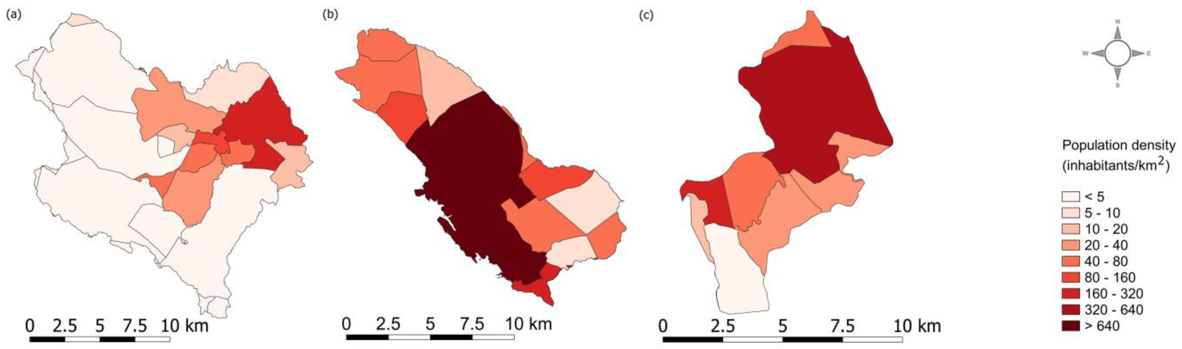
2.1. Study Areas
The effects of disaggregation are tested in three catchments in Croatia (Figure 2), each covered by different LULC datasets: the Gospić catchment (1), Zadar catchment (2) and Metković catchment (3). The selected catchments are partially urbanised, but with varying degrees of urbanisation. Furthermore, the predominant land use category also varies between the catchments.
Figure 2.
Location of the selected catchments.
The Gospić catchment area, with a surface area of 238 km2, stretches from the steep slopes of the Velebit Mountains in the west to the valley of the Lika River in the east. The altitudes vary from 550 m a.s.l. to 1500 m a.s.l. The administrative centre of the region, the town of Gospić with its 11,464 inhabitants [45], is located in the eastern part of the catchment. The dominant land use category is natural vegetation, i.e., forests and natural grasslands. Artificial land covers only small parts of the catchment (no more than 3%).
The Zadar catchment is the most urbanised of all three selected catchments: almost 25% of the catchment is covered with artificial land. It is located in Central Dalmatia and occupies an area of 118 km2. The largest centre of the catchment is the city of Zadar, which is located on the coast and has 70,829 inhabitants [45]. The highest altitude reaches 150 m a.s.l. and the predominant land use category is natural grassland.
The Metković catchment is located in the south of Croatia, on the border with Bosnia and Herzegovina. It is significantly smaller than the previously described catchments: its size is 52 km2. The altitude in some parts of the catchment is at sea level, while the highest altitude reaches 250 m a.s.l. The administrative centre of the region, the town of Metković, has 15,349 inhabitants [45]. The main economic activity is agriculture, which, together with wetlands, is also the predominant land use category. Artificial land covers less than 8% of the catchment area.
2.2. Copernicus LULC Data
The data used for the disaggregation are freely available data produced by the Copernicus Land Monitoring Service. It consists of two pan-European datasets, namely CORINE Land Cover (CLC) and the high-resolution imperviousness density (IMD) layer, and four LULC datasets within the local components that aim to provide detailed information for the specific regions, namely Coastal Zones (CZ), Natura 2000 (N2K), Riparian Zones and Urban Atlas (UA). The spatial and thematic level of detail varies between the datasets (Table 1 and Table 2).
Table 1.
Comparison of spatial characteristics of the available LULC datasets.
Table 2.
Comparison of thematic characteristics of the available LULC datasets.
The CLC dataset, which is most commonly used as a source of ancillary data, was not considered in this study due to its coarse spatial and thematic resolution compared to the other LULC datasets. Instead, the UA, CZ and N2K datasets were selected depending on the spatial coverage of the selected catchments.
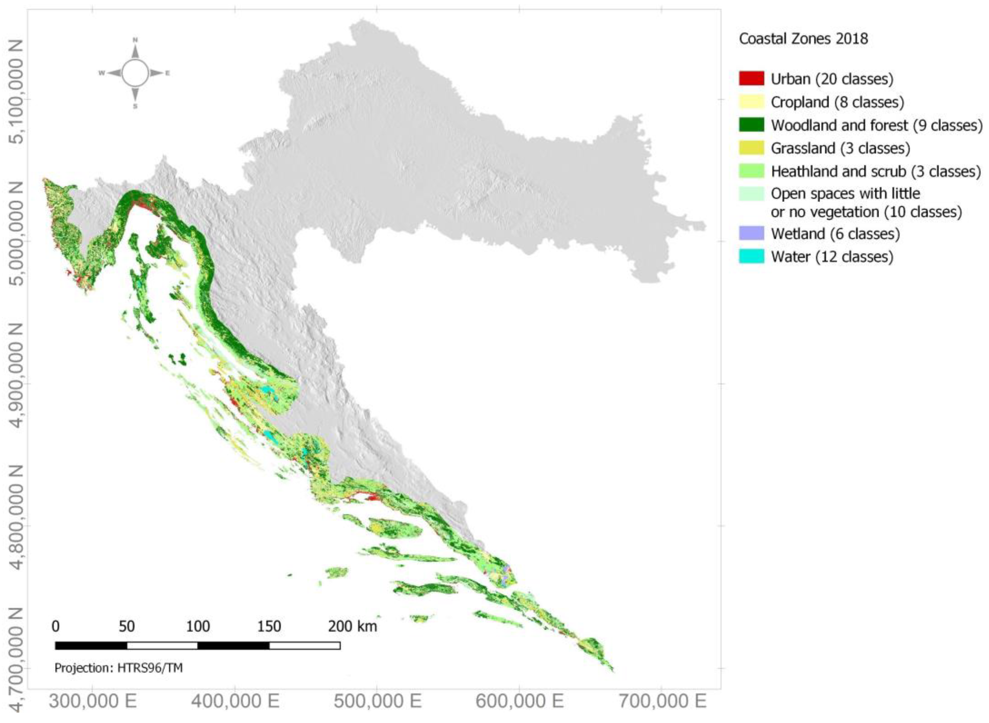
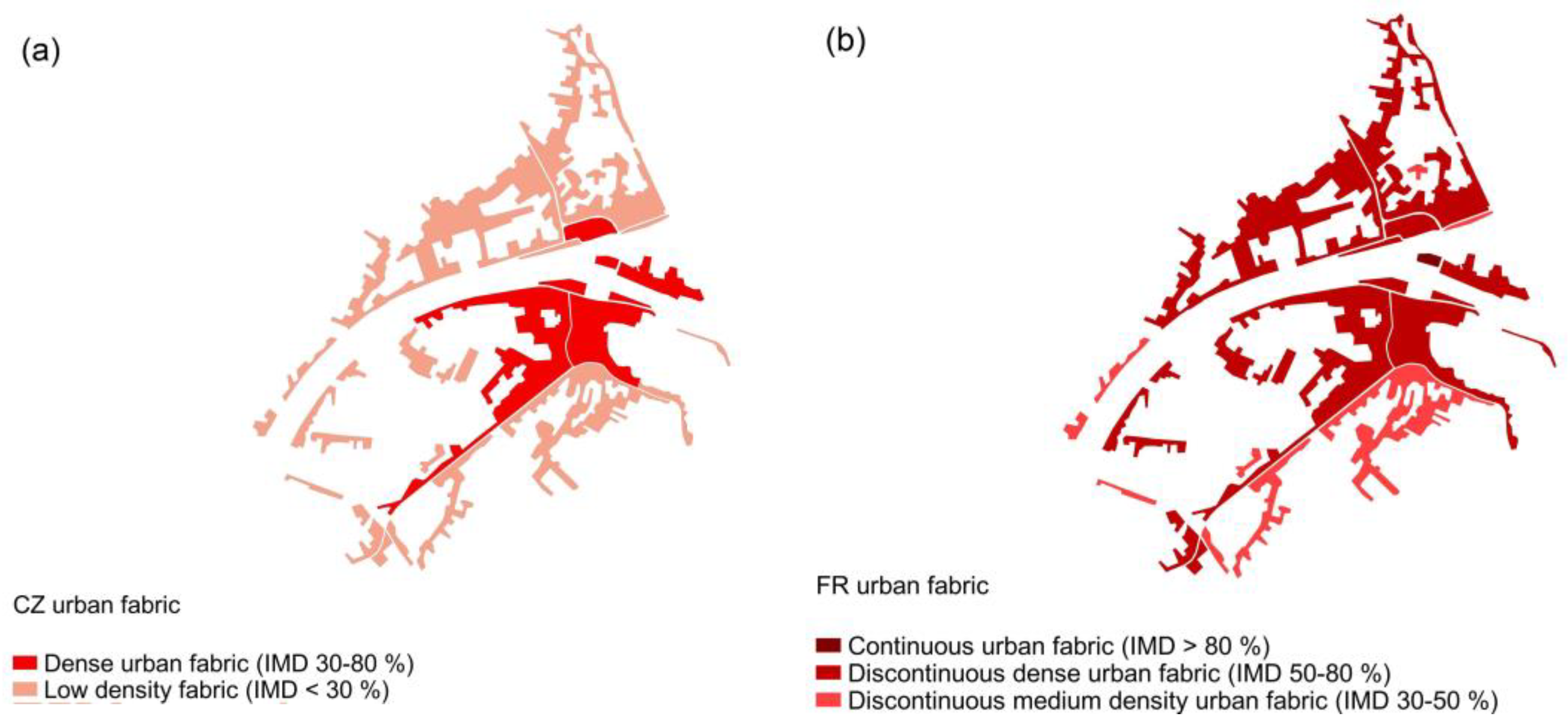
2.2.1. Coastal Zones (CZ 2018)
The requirements for spatial and thematic dynamics in coastal areas cannot be adequately met by the CLC method. Therefore, a detailed nomenclature based on the Mapping and Assessment of Ecosystems and their Services (MAES) typology [46] is proposed for the 10 km inland buffer zone and the seaward buffer zone along the coast. The database was first created for the reference year 2012 and updated in 2018. A hierarchical nomenclature similar to CLC is applied, but with greater thematic detail: the first level comprises eight LULC classes and the number of subsequent levels depends on the thematic unit. The total number of 71 classes (Figure 3) provides a higher level of detail that is required for efficient coastal zone management. The spatial accuracy is also greater compared to CLC: the minimum mapping unit is 0.5 ha and the minimum mapping width is 10 m.
Figure 3.
CZ 2018 1st nomenclature level for Croatia.
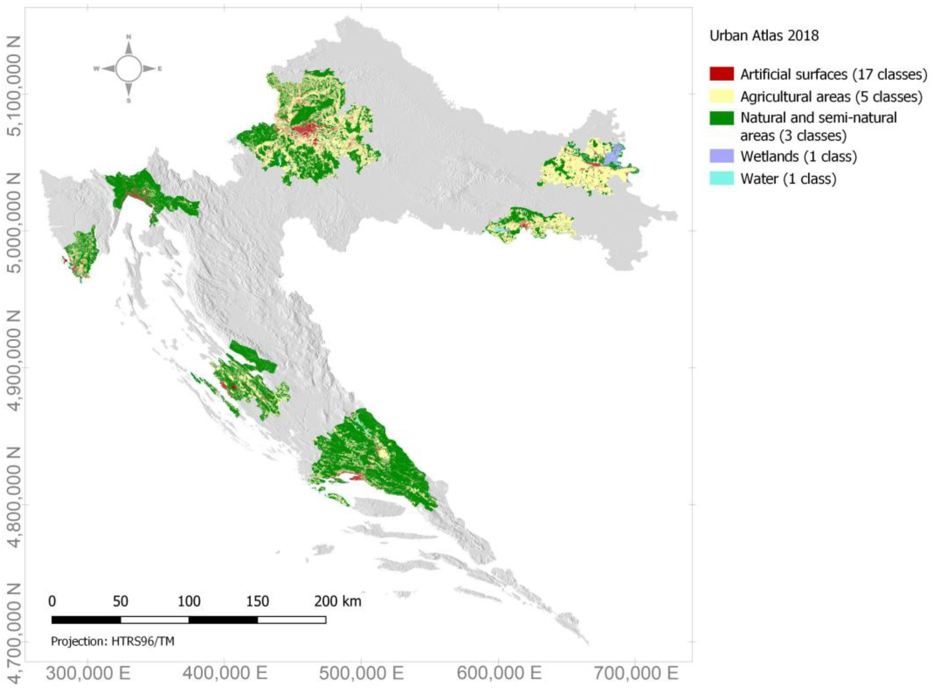
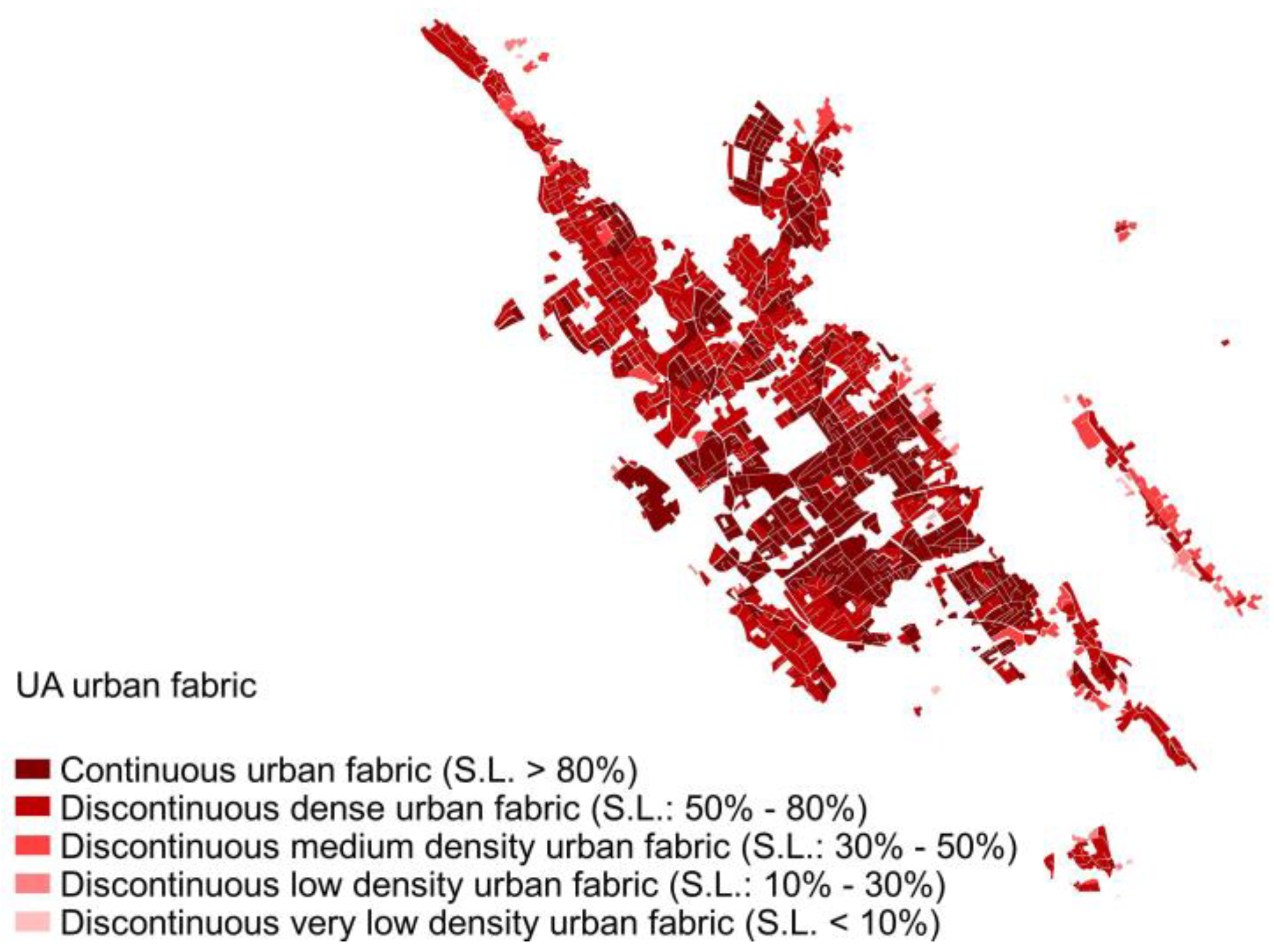
2.2.2. Urban Atlas (UA 2018)
The Urban Atlas is a collection of high-resolution land use data for urban areas across Europe for different reference years (2006, 2012, 2018). The first version contained detailed data for more than 300 functional urban areas (FUAs) of European cities. The latest update (Figure 4) includes data for more than 800 cities with more than 50,000 inhabitants [47]. The land use information comes from Earth observation systems and is complemented by additional data such as OpenStreetMap (OSM) or Commercial Off-The-Shelf (COST). The 1st level of nomenclature is taken from the CLC nomenclature, but the thematic level of detail in subsequent levels varies depending on the type of surface: artificial surfaces have the highest level of detail. With a minimum mapping unit of 0.25 ha in urban areas and 1 ha in rural areas, and a minimum mapping width of 10 m, it is the most detailed LULC dataset available for mapped European cities in a spatial context.
Figure 4.
UA 2018 1st nomenclature level for Croatia.
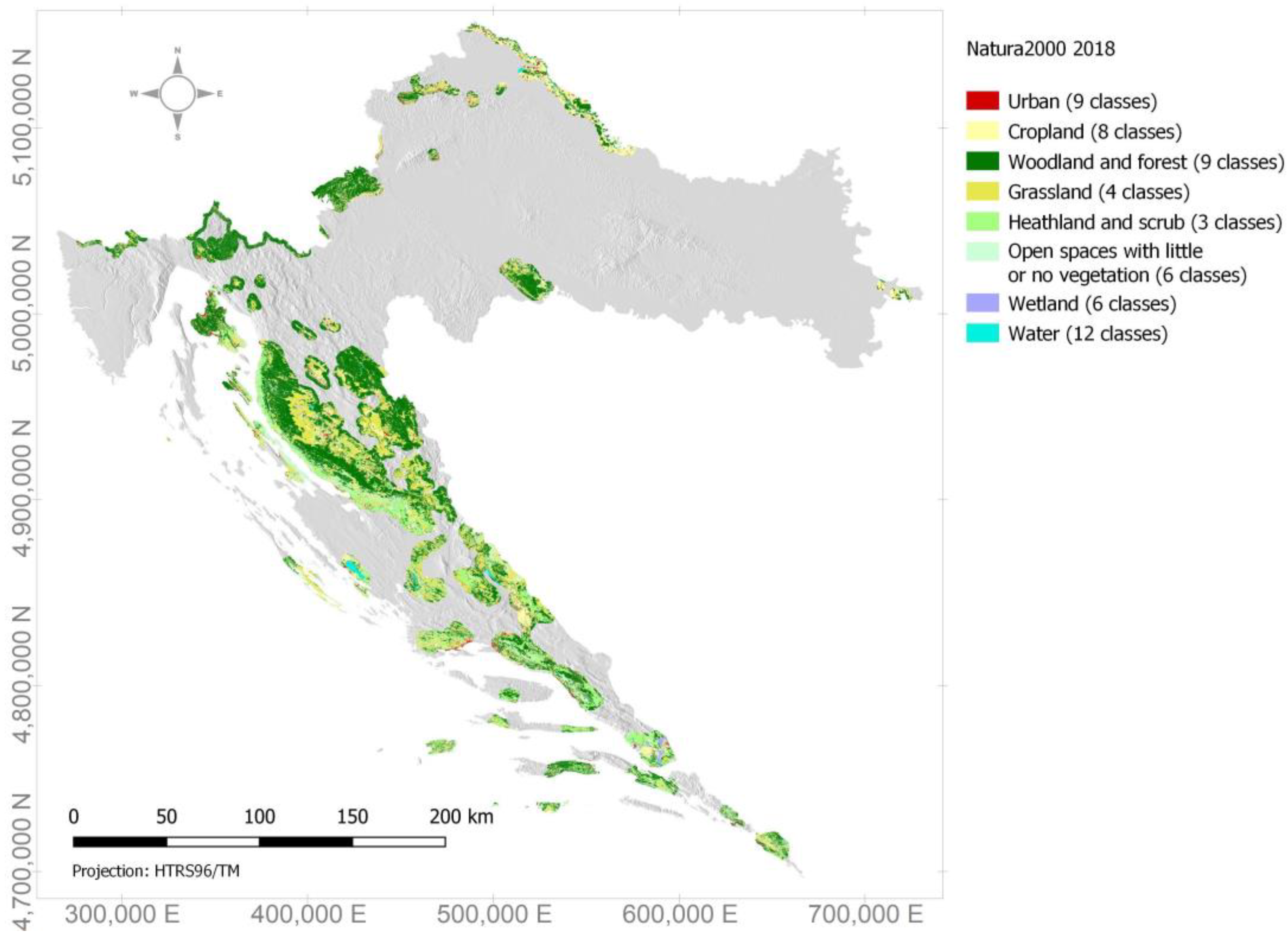
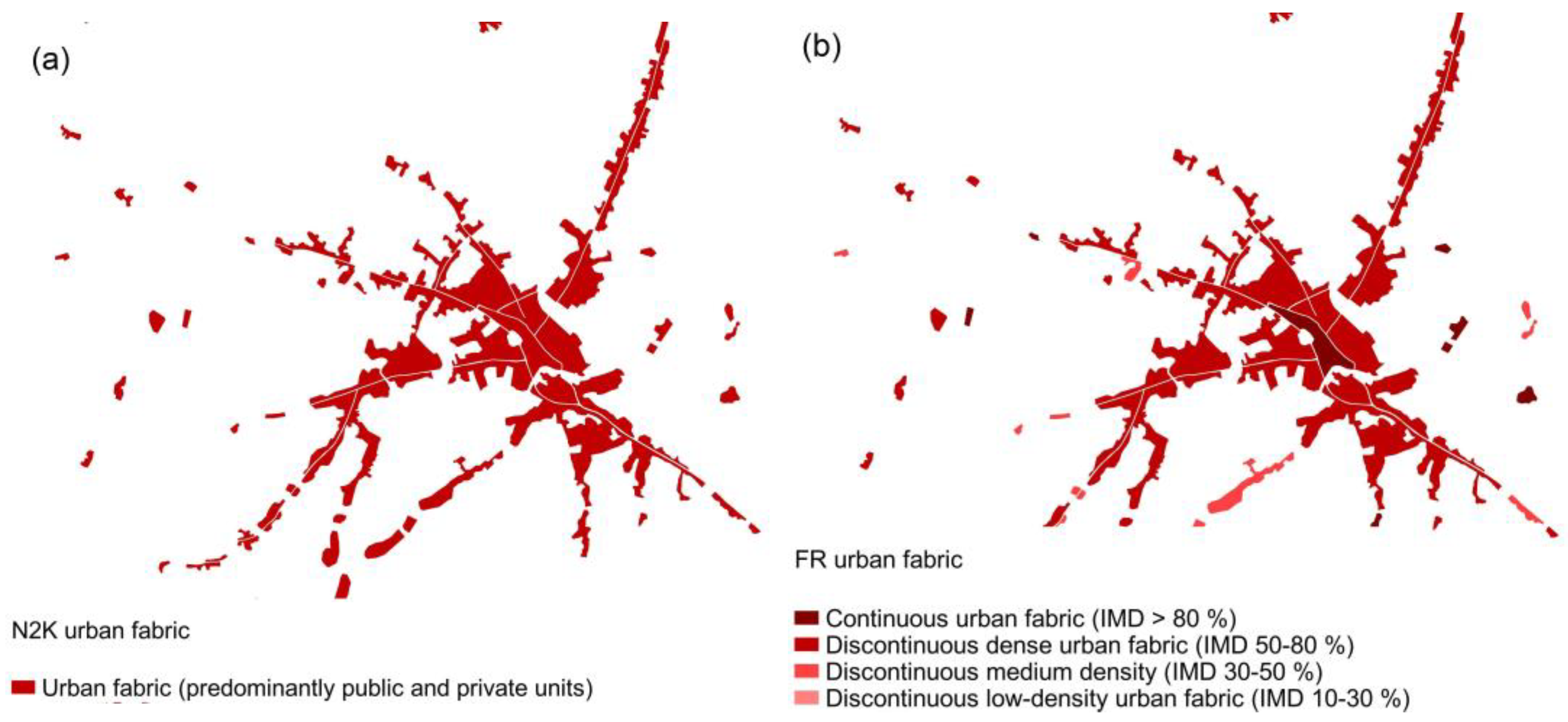
2.2.3. Natura 2000 (N2K 2018)
A detailed LULC classification for the sites that are recognised as Natura 2000 protected areas, including the 2 km buffer zone surrounding them, is provided by the N2K dataset. It was first created for the reference year 2006 and has since been updated twice, in 2012 and 2018, focusing specifically on areas with very high biodiversity values or potential [48]. Similar to the CZ nomenclature, the N2K nomenclature is based on the MAES specification for ecosystem types. At the 1st level, 8 thematic classes have been recognised and the number of subsequent levels depends on the thematic unit of importance for N2K differentiation: in total, it consists of 57 classes (Figure 5). The spatial accuracy is defined with a minimum mapping unit of 0.5 ha and a minimum mapping width of 10 m.
Figure 5.
N2K 2018 1st nomenclature level for Croatia.
2.3. Imperviousness Density (IMD 2018) and Imperviousness Built-Up (IBU 2018) Data
Imperviousness density describes the spatial distribution of surface imperviousness in built-up areas at a high spatial resolution (10 m) [49]. The level of the surface imperviousness represents the density of artificial soil sealing, which is based on the Normalised Difference Vegetation Index (NDVI) classification derived from remote sensing data (Figure 6). This dataset is not an LULC map in the strict sense, but provides valuable information that can be used for the thematic downscaling of urban LULC categories.
Figure 6.
IMD 2018 classification for Croatia.
Built-up areas are a subset of the IMD layer and represent only the IMD pixels with above-ground buildings [49]. Therefore, the attribute values of the layer are binary and only recognise built-up (value 1) or non-built-up (value 0) areas.
2.4. Census Data
The latest census data (from 2021) are aggregated and provided by the Croatian Bureau of Statistics at the settlement level [45]. The data used include the number of inhabitants in the settlements that are wholly or partly within the selected catchment areas (Figure 7).
Figure 7.
Choropleth maps of the population density in the settlements located in the selected catchments: (a) Gospić catchment; (b) Zadar catchment; (c) Metković catchment.
2.5. Methodological Framework
A spatial and thematic disaggregation of the LULC and census data was conducted in three phases: (1) data selection and preparation, (2) data disaggregation, (3) validation of the results.
- Phase 1: Data selection and preparation
As described earlier, three Copernicus LULC datasets are considered: CZ 2018, UA 2018 and N2K 2018. The selection of the appropriate dataset depends primarily on the spatial coverage of the selected catchments. Datasets that overlap with the catchment polygons are selected in terms of spatial and thematic characteristics (Table 1 and Table 2). The catchments’ imperviousness density characteristics are adopted from the high-resolution IMD layer.
Census data provide information on population size at the settlement level (administrative boundaries). In order to prepare the data for the population density disaggregation, the census data are mapped to the settlement polygons that are wholly or partially located in the selected catchments. The analysis of the change in the urban fabric between the cycle years of the LULC and IMD datasets, which are also available from the Copernicus Land Monitoring Service, shows that there is very little or no change in the catchments, so the temporal inconsistency between the LULC/IMD datasets and the census data is considered negligible.
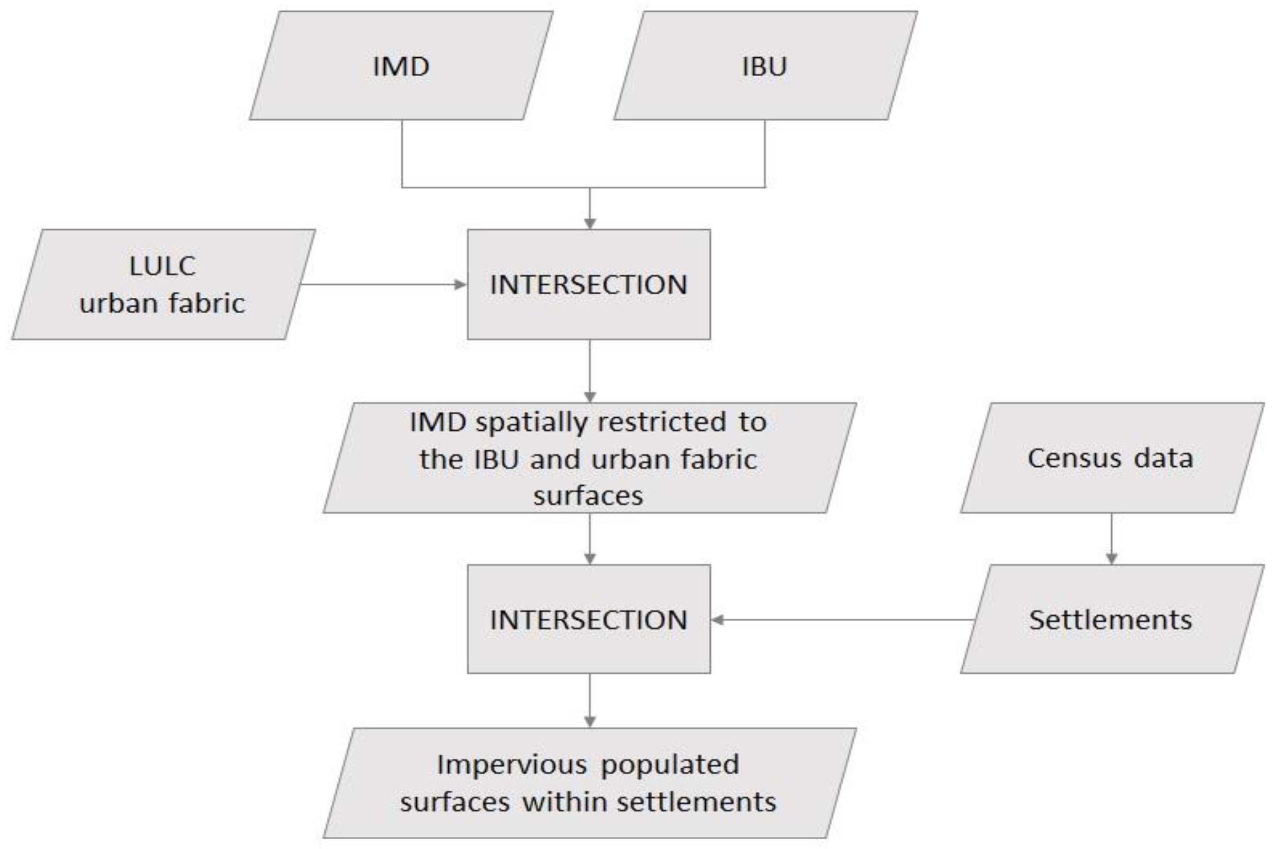
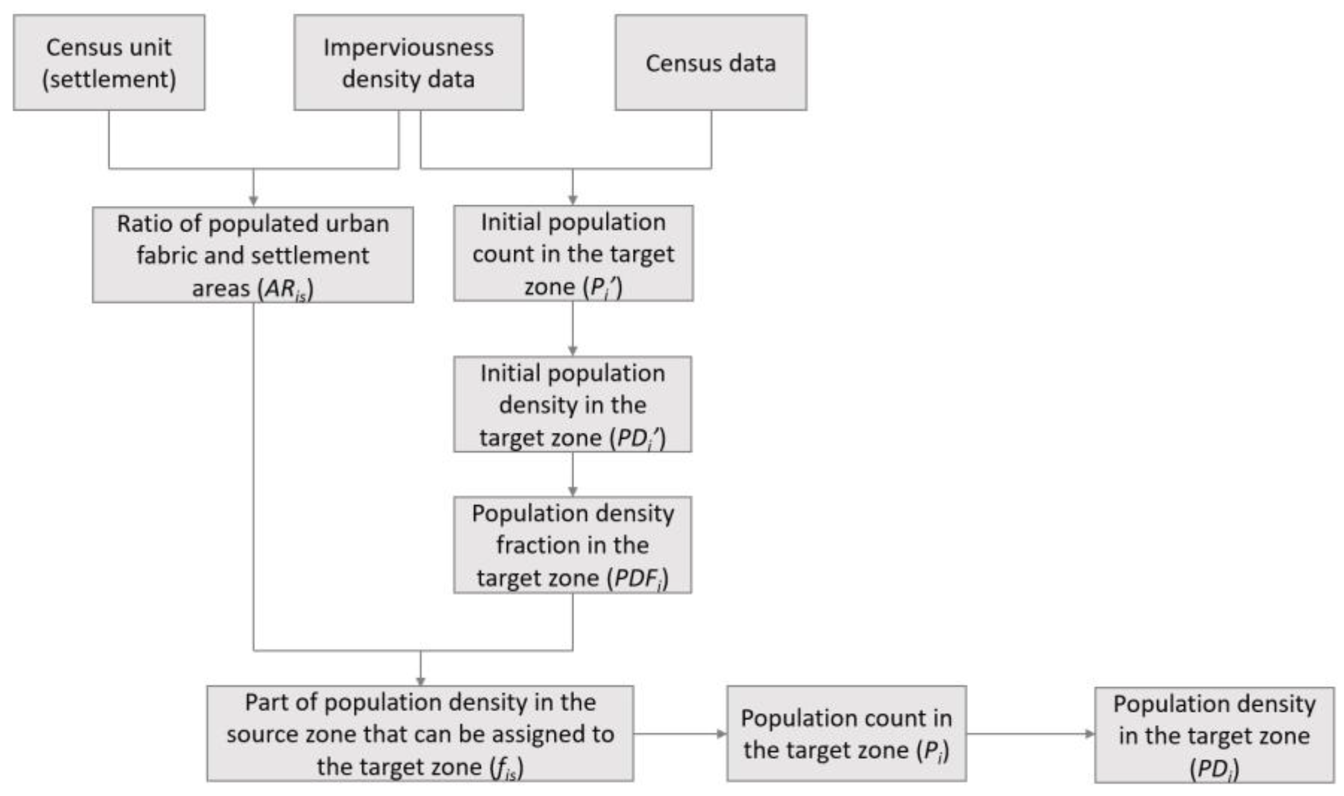
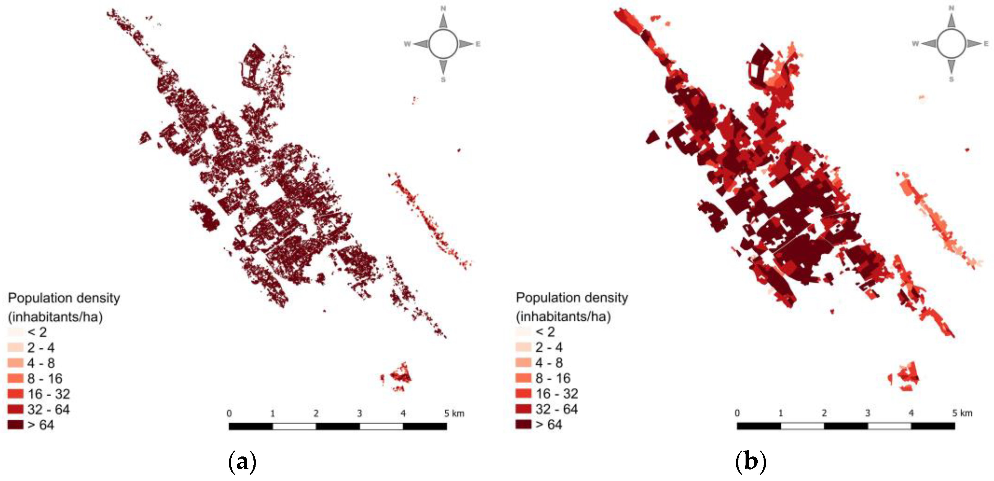
- Phase 2: Data disaggregation
In mapping, disaggregation is the process of regionalising the observed value using the auxiliary data [7]. Thus, the degree of disaggregation depends solely on the quality and availability of the auxiliary data. The flood risk assessment focuses primarily on artificial and agricultural land use categories and separates residential areas from commercial and industrial areas and transport infrastructure (Figure 1). The classification of the residential surfaces (urban structure in the LULC nomenclature) varies between the different LULC datasets and results in one (N2K), three (CZ) or five urban fabric classes (UA). Different LULC classifications lead to different values for Manning’s surface roughness.
The key parameter in urban structure classification in all LULC datasets is the impervious surface density, but with different thresholds: CZ uses three (1: IMD < 30%; 2: IMD = 30–80%; 3: IMD ≥ 80%), UA uses five (1: S.L. < 10%; 2: S.L. = 10–30%; 3: S.L. = 30–50%; 4: S.L. = 50–80%; 5: S.L. > 80%, where S.L. stands for the IMD sealing layer, i.e., the degree of soil sealing), while N2K has no threshold (only an aggregated urban fabric class). When the IMD layer is available, the urban fabric classes of the CZ and N2K datasets can be thematically disaggregated into five different classes using the UA classification thresholds (Table 3), which then provide the base geometry for estimating assets and people that are exposed to flooding at the meso level.
Table 3.
Urban classes of the available LULC nomenclatures (UA, CZ, N2K) and the result of thematic disaggregation (flood risk classification: FR).
The estimation of the population exposed to flooding at the level of the spatial unit, delineated using the thematic and spatial disaggregation procedure described earlier, is based on three basic assumptions:
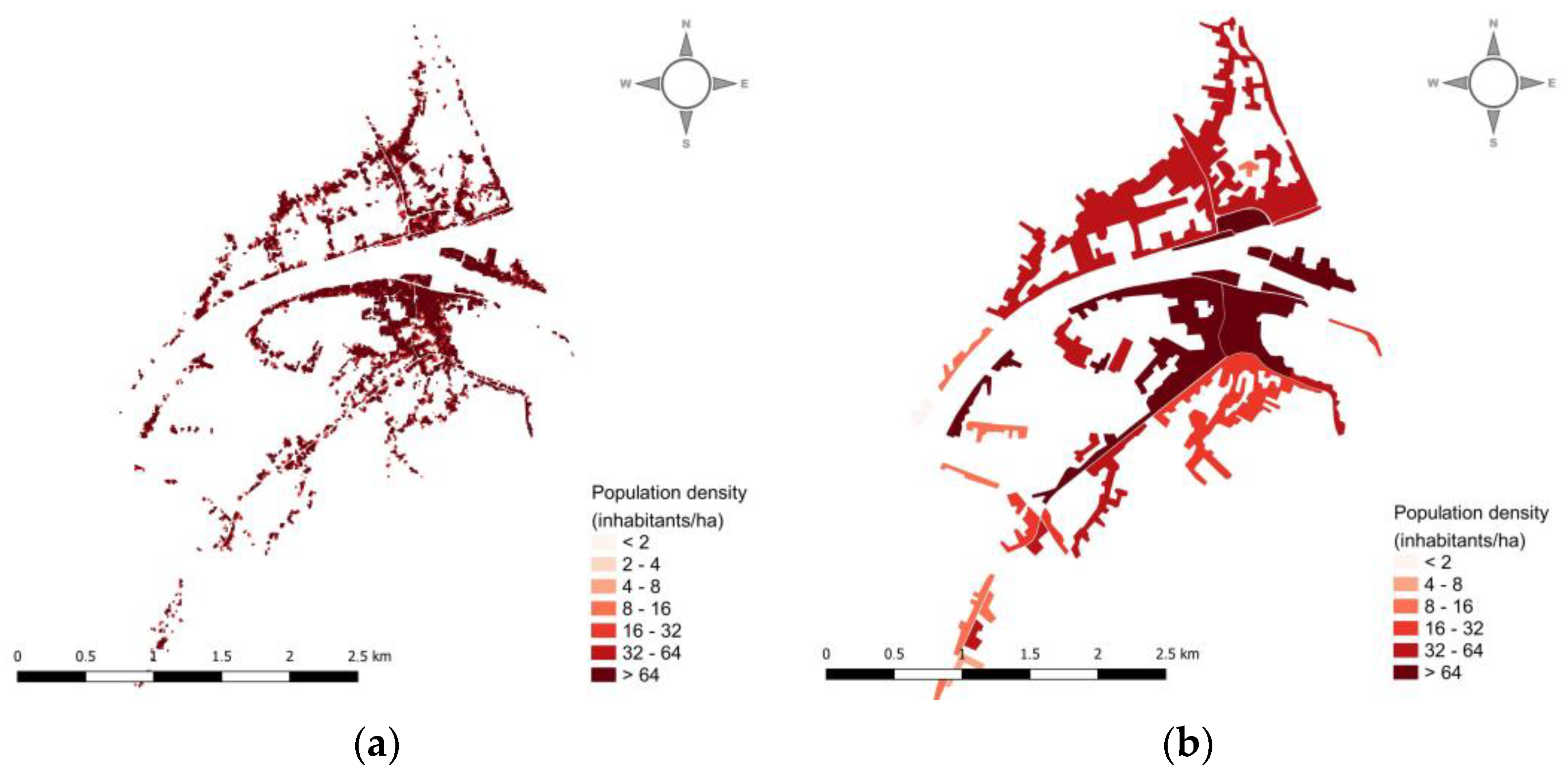
- Population density is related to the imperviousness density: IMD values are used as auxiliary data in estimating populations exposed to flooding;
- The population resides only in built-up areas [37]: to avoid the dissemination of the census data to areas occupied by non-residential buildings, built-up areas are removed from the IBU layer and used to spatially constrain the IMD distribution;
- The IMD values indicate the density of built-up areas: they consider the variability of built-up density and, consequently, the variability of a population.
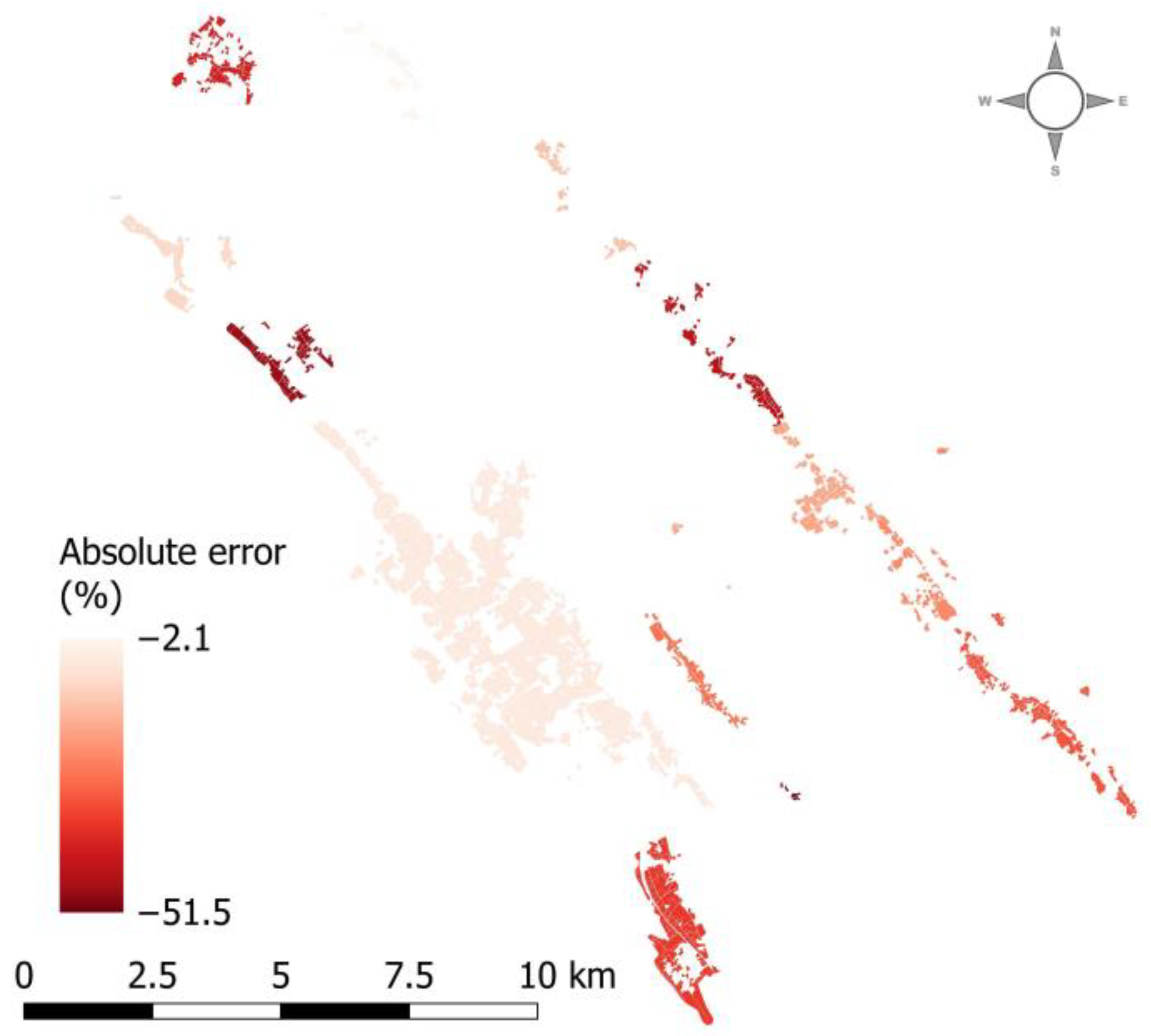
Census data are only available in the aggregated form that can be assigned to settlement polygons (Figure 8). In order to spatially disaggregate the data, i.e., to delineate the areas within settlements that can be populated, the IMD level, which is restricted to IBU areas only, is intersected with the urban fabric classes of the available LULC dataset. Finally, it is intersected with the settlement polygons that were previously assigned with the census data, i.e., the total number of inhabitants per settlement polygon. In this way, polygons that do not show settlement classes are excluded from further analysis and the population data are only assigned to areas that are exclusively occupied by residential buildings.
Figure 8.
Flow chart of the spatial data preparation.
The process of estimating population density for each disaggregated polygon is iterative. Each impervious populated polygon (target area) is assigned the initial number of inhabitants, which is calculated as a fraction of the total population count per settlement. The applied equation is commonly used in dasymetric population mapping applications, including population estimates in UA datasets [50,51]:
where P′i stands for the initial population in the target zone, i; Ps is the known population in the source zone, s (settlement); and Ai is the size of the target zone multiplied by the weighting coefficient, Wi. Originally, Wi refers to the average soil sealing value of the urban fabric class. The UA layer is only available for the Zadar catchment area and the population estimates correspond to the data collected by Eurostat for the year 2006 [51]. At the settlement level, the difference between the UA data and the 2021 census data varies, but in general, the UA estimates underestimate the 2021 census population (Figure 9). The differences are smaller (2.1%) in densely populated areas such as the city of Zadar, and increase (up to 51.5%) when the population density decreases, but the difference between the two datasets is not statistically significant (Table 4). Since the IMD value is available at the pixel level, instead of the average soil-sealing value of the LULC class for the urban fabric polygon, weighting coefficients can be derived from the IMD layer, i.e., the weighting coefficients are actually the IMD values, calculated as follows:
Figure 9.
Urban fabric aggregated absolute error of the UA estimated population with regard to the census data in the Zadar catchment.
Table 4.
Basic and t-test statistics of the census and the UA estimated population.
In general, the population count in spatially disaggregated LULC urban fabric polygons (target zones), Ps, is a fraction of the total population count in the settlement Ps derived from the census data [33,52]:
Fraction fis in the above equation marks the part of the population density in the source zone, s, that can be assigned to the target zone [37,53]:
The area ratio coefficient, ARis, ensures that higher weights are assigned to the impervious areas in order to link higher IMD values with higher population densities. The ratio of the populated urban fabric area, Ais, and total settlement area, As, is multiplied with the corresponding IMD value:
The population density fraction, PDFi, in Equation (4) allows for densely populated areas in the target zone to receive higher priority, i.e.,
With the area ratio coefficient and population density fraction included in calculations, inhabited areas with greater impervious density values are more likely to have a greater number of inhabitants. Finally, dividing the estimated population, Pi (Equation (3)), with the size of the target zone, i, Ai results in the spatial distribution of the population density:
The procedure is summarized and illustrated in Figure 10.
Figure 10.
Flow chart of the population density disaggregation procedure.
- Phase 3: Evaluation
To test the validity of the results, the root mean square error, RMSE, and percentage error, PE, are calculated for each analysed catchment:
where Ps and Pes are the actual and estimated populations in the census unit (settlement) and m is the number of settlements.
3. Results
Appropriate LULC datasets are selected for each catchment with respect to their extent and spatial characteristics (Table 5).
Table 5.
Available LULC datasets in selected catchments.
Two LULC datasets are available for the Zadar and Metković catchments: UA and CZ for the Zadar catchment and CZ and N2K for the Metković catchment. The spatial and thematic detail (Table 1 and Table 2) of the UA urban fabric classes is by far the best compared to other LUCL datasets, which is why it was selected for the Zadar catchment (Figure 11). The spatial characteristics of the CZ and N2K layers are identical, but the thematic characteristics of the urban structure classes are more detailed in the CZ layer.
Figure 11.
Details of the UA urban fabric classification in the Zadar catchment.
To test the accuracy of the thematic disaggregation of the UA urban fabric polygons and the appropriateness of using UA classification thresholds, the RMSE is calculated for each class in the catchments (Table 6). Classes with higher IMD values, occupying more than 80% of the total area of the urban fabric, fit the data better than the lowest IMD values. This is particularly evident for IMD values in the 50–80% range, which occupy almost 50% of the total area of the urban fabric. On the other hand, the RMSE is highest for the very-low-density discontinuous urban fabric (IMD values below 10%), which occupies only a small part of the urban fabric area (2.4%). The overall RMSE is less than one, indicating good agreement.
Table 6.
RMSE in the Zadar catchment.
The reclassification of urban fabric classes in the N2K and CZ layers selected for the Gospić and Metković catchments is carried out in respect of the average IMD values within the LULC urban fabric polygons (Table 3).
In the Gospić catchment, the thematic detail of the residential area is improved from one N2K urban fabric class to four FR urban fabric classes (Figure 12): most urban structure areas (75.4%) are classified as discontinuous dense urban fabrics, followed by medium-density urban fabric (17.1%), continuous urban fabric (7.3%) and discontinuous low-density urban fabric (<1%).
Figure 12.
Detail of the IMD corrected urban fabric classification in the Gospić catchment: (a) N2K urban fabric classification, (b) modified N2K urban fabric classification (FR classification).
In the Metković catchment area, two CZ urban fabric classes are reclassified into three FR urban fabric classes in terms of their average IMD value (Figure 13): the majority of urban areas are classified as discontinuous dense urban fabric classes (78.6%) and discontinuous medium-density urban fabric (20.9%), while only a small part is recognised as continuous urban fabric (<1%).
Figure 13.
Detail of the IMD corrected urban fabric classification in the Metković catchment: (a) CZ urban fabric classification, (b) modified CZ urban fabric classification (FR classification).
The spatial distribution of population density (inhabitants/ha) resulting from Equations (1)–(7) (Figure 14a, Figure 15a and Figure 16a) follows the spatial distribution of the IMD layer, which is restricted to the built-up areas within the LULC urban fabric classes. As expected, the highest densities occur in the areas associated with the LULC urban fabric polygons that are classified as continuous urban fabric (with IMD values above 80%) and discontinuous dense urban fabric (with IMD values within the interval 50–80%) (Figure 11, Figure 12 and Figure 13). To meet the requirements of small-scale assessment, the resulting pixel-wise population densities are aggregated based on the LULC urban fabric polygons (Figure 14b, Figure 15b and Figure 16b).
Figure 14.
Detail of the IMD derived population density classification in the Gospić catchment: (a) disaggregated to the pixel level, (b) aggregated to the FR polygon level.
Figure 15.
Detail of the IMD derived population density classification in the Metković catchment: (a) disaggregated to the pixel level, (b) aggregated to the FR polygon level.
Figure 16.
Detail of the IMD derived population density classification in the Zadar catchment: (a) disaggregated to the pixel level, (b) aggregated to the UA polygon level.
To validate the results, the root mean square error and percentage error for both the population count and population density are calculated using Equations (8) and (9) (Table 7). It should be noted that the results refer to the areas whose boundaries correspond to the administrative boundaries of the census units (settlements) that are wholly or partly within the boundaries of the catchment area.
Table 7.
Validation of the results.
As expected, the IMD values in combination with the UA dataset (Zadar catchment) result in the smallest RMSE and PE values. This is also the catchment with the highest population, especially in the central part where the city of Zadar is located, and the population density exceeds 64 inhabitants/ha. The Gospić catchment, as the least populated area, has slightly higher RMSE and PE values. The main economic activity in the Metković catchment is agriculture: the most represented LULC classes are different types of agriculture with individual farmhouses that are not recognised as residential due to the MMU of the dataset, which may lead to an incorrect population figure when estimating the population distribution in relation to the urban fabric polygons.
4. Discussion
The procedure described uses surface imperviousness data to disaggregate existing LULC urban fabric classes, as well as census data, which are normally only available in aggregated form at the settlement level. The main objective is to derive and process the basic spatial data that are necessary for estimating the exposure of assets and people to floods at the meso level and thus for assessing flood risk. In terms of exposure, the focus is primarily on the LULC classes of the urban fabric, which provide a detailed insight into the imperviousness characteristics that are critical for flood hazard and flood risk assessment at the meso level and the people living in these areas. The IMD thresholds used for the reclassification of urban fabrics in the available LULC datasets were taken from UA, clearly the most detailed dataset offered by the Copernicus Land Monitoring Service. The other datasets (N2K and CZ) are spatially harmonised (using the same MMU) and the nomenclature follows the same hierarchical procedure. However, the thematic detail of the urban fabric differs depending on the focus of the mapping procedure: CZ focuses on monitoring the marine coastline and provides information on the impact of anthropogenic activities on the marine environment, while the purpose of the N2K data is to assess the effectiveness of the preservation of Natura 2000 sites. In general, the differentiation in the different levels of the imperviousness density within the urban environment is not so much in focus, and both end up with far fewer classes of urban fabric than the UA dataset (Table 3), which is not suitable for flood risk assessment, and is primarily focused on urban and agricultural areas and aims to assess the adverse consequences of flooding at the meso level.
The advantage of the described thematic disaggregation of the LULC urban fabric is its simplicity, as only the available high-resolution IMD is used as auxiliary data. Based on the assumption that a higher imperviousness density indicates a higher building density and greater asset value, the reclassification of the existing urban classes in terms of the IMD value allows for a more detailed analysis of the assets at risk. In this regard, the proposed disaggregation of the LULC thematic urban fabric information is a step forward to adjust the data and extract adequate information from the available data. On the other hand, in terms of spatial characteristics, the disaggregated data are still within the spatial boundaries of the urban fabric polygons of the LULC dataset used, so further improvements are needed to improve the spatial detail and, in particular, to adjust the boundaries of the urban fabric polygons.
Similar to the LULC data, census data are usually only available at an aggregated level (e.g., settlement) and are not detailed enough to meet the meso-level requirements. In recent decades, many approaches to disaggregating population density data have been proposed, including areal interpolation techniques and dasymetric mapping. The disaggregation approach described in this study is based on the dasymetric method proposed by Mennis [52] and Mennis and Hultgren [33], which defines the relationship between the statistical component being mapped (census data) and the auxiliary data used to assign appropriate value classes to the residential areas (urban fabric classes in the selected LULC layer). However, instead of using aggregate auxiliary classes (i.e., the average imperviousness density of each LULC urban fabric class), we propose to use the actual IMD values derived from the IMD layer and establish the relationship between population density and mapped IMD. With a spatial resolution that is detailed enough for meso-level assessment, the IMD layer provides sufficient information to disaggregate the population data at a finer scale. In contrast to choropleth mapping (Figure 7), the main objective of the described approach is to distribute census data to areas that are actually inhabited by residents, rather than allocating population density to the entire administrative unit (settlement). The approach is based on the assumption that higher values for impervious density tend to indicate a higher density of residential development and, consequently, are more likely to be inhabited by residents. To avoid assigning population density values to areas with high IMD values that are not residential (e.g., industrial or commercial buildings, roads), the IMD values are spatially limited to the selected LULC urban fabric polygons. In other words, the distribution of population density is determined based on the density of imperviousness and the proportion of the area in the settlements that can be considered residential.
The population distribution presented in this paper is a significant improvement over the currently available population data for Croatia. Figure 17 shows the currently available distribution of population data from the world’s largest population dataset, WorldPop [54]. The dataset is compiled based on the 2020 census- or projection-based estimates for 2020 [39]. In terms of flood risk assessment, the dataset is suitable for macro-level assessment, but at the meso level, such a coarse resolution cannot provide satisfactory estimates for flood exposure and flood damage analysis. The proposed approach not only improves the spatial resolution of population distribution, but is also an improvement in terms of thematic distribution: it allows for pixel-based estimates based on the latest census data instead of projections.
Figure 17.
Detail of the WorldPop population density at a 100 km resolution in the selected catchments: (a) Gospić catchment; (b) Zadar catchment; (c) Metković catchment.
5. Conclusions
Estimating the exposure of the elements at risk, both assets and people, is the key element of flood risk assessment. The process relates the flood hazard to the vulnerability of the exposed elements to estimate the damage and, ultimately, the flood risk. As mentioned above, the assessment is subject to many uncertainties, often related to the data used. Most of the data that are already available are suitable for mapping flood risks at the macro level. However, for flood risk assessment at the meso (and micro) scale, sufficiently detailed data are often lacking, forcing researchers to combine available assets and census data with auxiliary information. Disaggregation techniques based on finding the functional relationship between the aggregated and the auxiliary data (most commonly, the imperviousness density) are one way to deal with the lack of detail. The aim of this research was to propose a method that disaggregates exposure data (both for assets and residents) at a meso level, using census data collected at the aggregated level (settlements) and available LULC datasets, namely Coastal Zones, Natura 2000 and Urban Atlas, as well as pixel-based IMD information as auxiliary data.
The main strength of the presented approach is primarily the use of the already available data (Copernicus Land Monitoring Service LULC and IMD data) and the latest census data, so that no additional data collection is required, which can be very time-consuming and costly. Although the thematic disaggregation of urban fabric classes is spatially limited by the polygon boundaries of the selected LULC dataset, which means that the accuracy at the polygon boundaries depends on the accuracy of the original LULC dataset, the information on the urban fabric classes and, consequently, the exposure of the elements at risk is greatly improved. In terms of population density disaggregation, pixel-based IMD data allow for better sensitivity to the variability of population density within the target zones and improve the accuracy of the estimation of weights for the different IMD levels. The result is a population density that is spatially disaggregated down to the specific urban fabric polygons, which allows for an estimation of the people that are exposed to flooding at the catchment level.
Limitations of the Proposed Method and Further Improvement
As described, the approach is specifically designed for countries where census data are available, and its main objective is to provide the population data that are needed for flood exposure analysis. If no census data are available, projection data, such as WorldPop, must be used, but with certain methodological adjustments to the disaggregation procedure described.
Apart from exposure, asset damage is highly dependent on the depth–damage information available. The thematic detail of the depth–damage curves that are commonly used in mesoscale flood risk assessment is relatively low in terms of land use categories. Built-up areas are classified into five value classes: residential, commercial, industrial, transport and infrastructure—roads. The disaggregated LULC urban fabric described earlier recognises five residential classes depending on the percentage of impervious surfaces. However, the depth–damage curves combine the residential classes into one category, which reduces the accuracy of damage assessment in built-up areas and could be misleading when assessing the effectiveness of flood protection measures.
The greatest flood damage occurs in urban areas. In this paper, the approach described is limited to estimating population density that only considers residents, i.e., we have only considered the exposure of residents and residential assets. Daily and seasonal migrations are not considered. Further improvements should focus on including other urban (e.g., industrial, commercial) and agricultural classes, and including non-residents who might be exposed to flooding (e.g., tourists, workers). Extensive sampling is also recommended to improve the validation of the disaggregated data (both assets and population).
One of the assumptions on which the approach is based is the use of IMD values as an indicator of building density. To estimate the exposure of residents in even more detail, building heights can also be taken into account as one of the indicators of population density (the higher the building, the denser the population) by using the difference between the high-resolution digital elevation model (DEM) and the digital surface model (DSM) as an indicator of the height of the building.
Author Contributions
Conceptualization, B.H. and N.K.; methodology, B.H. and N.K.; software, B.H. and N.K.; validation, B.H.; formal analysis, B.H. and N.K.; investigation, B.H. and N.K.; resources, B.H. and N.K.; data curation, B.H.; writing—original draft preparation, B.H.; writing—review and editing, B.H. and N.K.; visualization, B.H.; supervision, B.H.; project administration, N.K.; funding acquisition, N.K. All authors have read and agreed to the published version of the manuscript.
Funding
This research was funded by the Italy–Croatia cross-border cooperation program 2014–2020 under the Interreg project, the Strategic development of flood management (STREAM). This research was also funded by the University of Rijeka Projects: uniri-tehnic-18-129 and uniri-tehnic-18-54.
Data Availability Statement
Coastal Zones land cover, Natura 2000 land cover, Urban Atlas land cover, imperviousness density and imperviousness built-up data from the Copernicus Land Monitoring Service can be accessed at https://land.copernicus.eu/ (accessed on 21 September 2023). Census 2021 data from the Croatian Bureau of Statistics can be accessed at https://dzs.gov.hr/ (accessed on 21 September 2023). Population data from the WorldPop project can be accessed at https://www.worldpop.org/ (accessed on 24 October 2023).
Conflicts of Interest
The authors declare no conflict of interest.
Appendix A
Table A1.
Comparison of the urban and agricultural classes of the available LULC nomenclatures.
Table A1.
Comparison of the urban and agricultural classes of the available LULC nomenclatures.
| CORINE Based Level 1 | MAES Based Level 1 | CLC | UA | CZ | N2K |
|---|---|---|---|---|---|
| Artificial surfaces | Urban | Continuous urban fabric | Continuous urban fabric (SL > 80%) | Continuous urban fabric (IMD > 80%) | Urban fabric (predominantly public and private units) |
| Discontinuous urban fabric | Discontinuous dense urban fabric (SL 50–80%) | Dense urban fabric (IMD 30–80%) | |||
| Discontinuous medium-density urban fabric (SL 30–50%) | |||||
| Discontinuous low-density urban fabric (SL 10–30%) | Low-density fabric (IMD < 30%) | ||||
| Discontinuous very-low-density urban fabric (SL < 10%) | |||||
| Industrial or commercial units | Industrial, commercial, public, military and private units | Industrial, commercial, public and military units (other) | Industrial, commercial and military units | ||
| Nuclear energy plants and associated land | |||||
| Road and rail networks and associated land | Fast transit roads and associated land | Road networks and associated land | Road networks and associated land | ||
| Other roads and associated land | |||||
| Railways and associated land | Railways and associated land | Railways and associated land | |||
| Port areas | Port areas | Cargo ports | Port areas | ||
| Passenger ports | |||||
| Fishing ports | |||||
| Naval ports | |||||
| Marinas | |||||
| Local multi-functional harbours | |||||
| Shipyards | |||||
| Airports | Airports | Airports and associated land | Airports and associated land | ||
| Mineral extraction sites | Mineral extraction and dump sites | Mineral extraction sites | Mineral extraction sites, dump and construction sites | ||
| Dump sites | Dump sites | ||||
| Construction sites | Construction sites | Construction sites | |||
| - | Land without current use | Land without current use | Land without current use | ||
| Green urban areas | Green urban areas | Green urban, sports and leisure facilities | Green urban, sports and leisure facilities | ||
| Sport and leisure facilities | Sport and leisure facilities | ||||
| Agricultural areas | Cropland | Non-irrigated arable land | Arable land (crops) | Arable irrigated and non-irrigated land | Arable irrigated and non-irrigated land |
| Permanently irrigated arable land | |||||
| Rice fields | |||||
| - | - | Greenhouses | Greenhouses | ||
| Vineyards | Permanent crops | Vineyards, fruit trees and berry plantations | Vineyards, fruit trees and berry plantations | ||
| Fruit trees and berry plantations | |||||
| Olive groves | Olive groves | Olive groves | |||
| Pasture | Pastures | Annual crops associated with permanent crops | Annual crops associated with permanent crops | ||
| Annual crops associated with permanent crops | - | ||||
| Complex cultivation patterns | Complex and mixed cultivation | Complex cultivation patterns | Complex cultivation patterns | ||
| Land principally occupied by agriculture with significant areas of natural vegetation | - | Land principally occupied by agriculture with significant areas of natural vegetation | Land principally occupied by agriculture with significant areas of natural vegetation | ||
| Agro-forestry areas | - | Agro-forestry areas | Agro-forestry areas |
References
- Rentschler, J.; Salhab, M.; Jafino, B.A. Flood Exposure and Poverty in 188 Countries. Nat. Commun. 2022, 13, 3527. [Google Scholar] [CrossRef] [PubMed]
- Tellman, B.; Sullivan, J.A.; Kuhn, C.; Kettner, A.J.; Doyle, C.S.; Brakenridge, G.R.; Erickson, T.A.; Slayback, D.A. Satellite Imaging Reveals Increased Proportion of Population Exposed to Floods. Nature 2021, 596, 80–86. [Google Scholar] [CrossRef] [PubMed]
- Yang, L.; Smith, J.A.; Wright, D.B.; Baeck, M.L.; Villarini, G.; Tian, F.; Hu, H. Urbanization and Climate Change: An Examination of Nonstationarities in Urban Flooding. J. Hydrometeorol. 2013, 14, 1791–1809. [Google Scholar] [CrossRef]
- Paprotny, D.; Sebastian, A.; Morales-Nápoles, O.; Jonkman, S.N. Trends in Flood Losses in Europe over the Past 150 Years. Nat. Commun. 2018, 9, 1985. [Google Scholar] [CrossRef]
- CRED 2021 Disasters in Numbers. Brussels. 2022. Available online: https://www.un-spider.org/news-and-events/news/cred-publication-2021-disasters-numbers (accessed on 1 March 2023).
- EEA Economic Losses and Fatalities from Weather- and Climate-Related Events in Europe. 2022. Available online: https://www.eea.europa.eu/publications/economic-losses-and-fatalities-from/economic-losses-and-fatalities-from (accessed on 15 March 2023).
- Merz, B.; Kreibich, H.; Schwarze, R.; Thieken, A. Review Article “Assessment of Economic Flood Damage”. Nat. Hazards Earth Syst. Sci. 2010, 10, 1697–1724. [Google Scholar] [CrossRef]
- De Moel, H.; Jongman, B.; Kreibich, H.; Merz, B.; Penning-Rowsell, E.; Ward, P.J. Flood Risk Assessments at Different Spatial Scales. Mitig. Adapt. Strateg. Glob. Chang. 2015, 20, 865–890. [Google Scholar] [CrossRef] [PubMed]
- Gabriels, K.; Willems, P.; Van Orshoven, J. A Comparative Flood Damage and Risk Impact Assessment of Land Use Changes. Nat. Hazards Earth Syst. Sci. 2022, 22, 395–410. [Google Scholar] [CrossRef]
- Krvavica, N.; Šiljeg, A.; Horvat, B.; Panđa, L. Pluvial Flash Flood Hazard and Risk Mapping in Croatia: Case Study in the Gospić Catchment. Sustainability 2023, 15, 1197. [Google Scholar] [CrossRef]
- Tsakiris, G. Flood Risk Assessment: Concepts, Modelling, Applications. Nat. Hazards Earth Syst. Sci. 2014, 14, 1361–1369. [Google Scholar] [CrossRef]
- Meyer, V.; Becker, N.; Markantonis, V.; Schwarze, R.; van den Bergh, J.C.J.M.; Bouwer, L.M.; Bubeck, P.; Ciavola, P.; Genovese, E.; Green, C.; et al. Review Article: Assessing the Costs of Natural Hazards—State of the Art and Knowledge Gaps. Nat. Hazards Earth Syst. Sci. 2013, 13, 1351–1373. [Google Scholar] [CrossRef]
- Wagenaar, D.J.; de Bruijn, K.M.; Bouwer, L.M.; de Moel, H. Uncertainty in Flood Damage Estimates and Its Potential Effect on Investment Decisions. Nat. Hazards Earth Syst. Sci. 2016, 16, 1–14. [Google Scholar] [CrossRef]
- Messner, F.; Meyer, V. Flood Damage, Vulnerability and Risk Perception—Challenges for Flood Damage Research. In Flood Risk Management: Hazards, Vulnerability and Mitigation Measures; Schanze, J., Zeman, E., Marsalek, J., Eds.; Springer: Dordrecht, The Netherlands, 2006; pp. 149–167. [Google Scholar]
- Messner, F.; Penning-Rowsell, E.; Green, C.; Meyer, V.; Tunstall, S.; van der Veen, A. Evaluating Flood Damages: Guidance and Recommendations on Principles and Methods, T09-06-01; FLOOD Site Project Report: Wallingford, UK, 2007. [Google Scholar]
- De Moel, H.; Aerts, J.C.J.H. Effect of Uncertainty in Land Use, Damage Models and Inundation Depth on Flood Damage Estimates. Nat. Hazards 2011, 58, 407–425. [Google Scholar] [CrossRef]
- Hall, J.W.; Sayers, P.B.; Dawson, R.J. National-Scale Assessment of Current and Future Flood Risk in England and Wales. Nat. Hazards 2005, 36, 147–164. [Google Scholar] [CrossRef]
- Barredo, J.I.; de Roo, A.; Lavalle, C. Flood Risk Mapping at European Scale. Water Sci. Technol. 2007, 56, 11–17. [Google Scholar] [CrossRef]
- Fleischmann, A.; Paiva, R.; Collischonn, W. Can Regional to Continental River Hydrodynamic Models Be Locally Relevant? A Cross-Scale Comparison. J. Hydrol. X 2019, 3, 100027. [Google Scholar] [CrossRef]
- Kreibich, H.; Seifert, I.; Merz, B.; Thieken, A.H. Development of FLEMOcs—A New Model for the Estimation of Flood Losses in the Commercial Sector. Hydrol. Sci. J. 2010, 55, 1302–1314. [Google Scholar] [CrossRef]
- Krvavica, N.; Horvat, B.; Ružić, I.; Tadić, A.; Roland, V.; Šiljeg, A.; Marić, I.; Šiljeg, S.; Domazetović, F.; Panđa, L.; et al. Experiences with Pluvial Flood Risk Mapping in Croatia at Multiple Spatial Scales. In Proceedings of the 40th IAHR World Congress, Vienna, Austria, 21–25 August 2023; IAHR: Vienna, Austria, 2023. [Google Scholar]
- Lin, J.; Zhang, W.; Wen, Y.; Qiu, S. Evaluating the Association between Morphological Characteristics of Urban Land and Pluvial Floods Using Machine Learning Methods. Sustain. Cities Soc. 2023, 99, 104891. [Google Scholar] [CrossRef]
- McBean, E.; Fortin, M.; Gorrie, J. A Critical Analysis of Residential Flood Damage Estimation Curves. Can. J. Civil. Eng. 1986, 13, 86–94. [Google Scholar] [CrossRef]
- Smith, D.I. Flood Damage Estimation—A Review of Urban Stage-Damage Curves and Loss Functions. Water SA 1994, 20, 231–238. [Google Scholar]
- Jongman, B.; Kreibich, H.; Apel, H.; Barredo, J.I.; Bates, P.D.; Feyen, L.; Gericke, A.; Neal, J.; Aerts, J.C.J.H.; Ward, P.J. Comparative Flood Damage Model Assessment: Towards a European Approach. Nat. Hazards Earth Syst. Sci. 2012, 12, 3733–3752. [Google Scholar] [CrossRef]
- Thieken, A.H.; Müller, M.; Kreibich, H.; Merz, B. Flood Damage and Influencing Factors: New Insights from the August 2002 Flood in Germany. Water Resour. Res. 2005, 41, W12430. [Google Scholar] [CrossRef]
- Pistrika, A.; Tsakiris, G.; Nalbantis, I. Flood Depth-Damage Functions for Built Environment. Environ. Process. 2014, 1, 553–572. [Google Scholar] [CrossRef]
- Shah, M.A.R.; Rahman, A.; Chowdhury, S.H. Challenges for Achieving Sustainable Flood Risk Management. J. Flood Risk Manag. 2018, 11, S352–S358. [Google Scholar] [CrossRef]
- Huizinga, J.; de Moel, H.; Szewczyk, W. Global Flood Depth-Damage Functions: Methodology and the Database with Guidlines; Publications Office of the European Union: Luxembourg, 2017. [Google Scholar]
- Balogun, A.-L.; Mohd Said, S.A.; Sholagberu, A.T.; Aina, Y.A.; Althuwaynee, O.F.; Aydda, A. Assessing the Suitability of GlobeLand30 for Land Cover Mapping and Sustainable Development in Malaysia Using Error Matrix and Unbiased Area Estimation. Geocarto Int. 2022, 37, 1607–1627. [Google Scholar] [CrossRef]
- Chen, J.; Cao, X.; Peng, S.; Ren, H. Analysis and Applications of GlobeLand30: A Review. ISPRS Int. J. Geoinf. 2017, 6, 230. [Google Scholar] [CrossRef]
- Gallego, F.J.; Batista, F.; Rocha, C.; Mubareka, S. Disaggregating Population Density of the European Union with CORINE Land Cover. Int. J. Geogr. Inf. Sci. 2011, 25, 2051–2069. [Google Scholar] [CrossRef]
- Mennis, J.; Hultgren, T. Intelligent Dasymetric Mapping and Its Application to Areal Interpolation. Cartogr. Geogr. Inf. Sci. 2006, 33, 179–194. [Google Scholar] [CrossRef]
- Gallego, F.J. A Population Density Grid of the European Union. Popul. Environ. 2010, 31, 460–473. [Google Scholar] [CrossRef]
- Briggs, D.J.; Gulliver, J.; Fecht, D.; Vienneau, D.M. Dasymetric Modelling of Small-Area Population Distribution Using Land Cover and Light Emissions Data. Remote Sens. Environ. 2007, 108, 451–466. [Google Scholar] [CrossRef]
- Eicher, C.L.; Brewer, C.A. Dasymetric Mapping and Areal Interpolation: Implementation and Evaluation. Cartogr. Geogr. Inf. Sci. 2001, 28, 125–138. [Google Scholar] [CrossRef]
- Starmans, S.M. Spatial Disaggregation of Population Data onto Urban Footprint Data; Leopold-Franzens-Universität Innsbruck: Innsbruck, Austria, 2014. [Google Scholar]
- Wu, C.; Murray, A.T. A Cokriging Method for Estimating Population Density in Urban Areas. Comput. Environ. Urban. Syst. 2005, 29, 558–579. [Google Scholar] [CrossRef]
- Stevens, F.R.; Gaughan, A.E.; Linard, C.; Tatem, A.J. Disaggregating Census Data for Population Mapping Using Random Forests with Remotely-Sensed and Ancillary Data. PLoS ONE 2015, 10, e0107042. [Google Scholar] [CrossRef] [PubMed]
- Tatem, A.J. WorldPop, Open Data for Spatial Demography. Sci. Data 2017, 4, 170004. [Google Scholar] [CrossRef] [PubMed]
- Sherba, J.T.; Sleeter, B.M.; Davis, A.W.; Parker, O. Downscaling Global Land-Use/Land-Cover Projections for Use in Region-Level State-and-Transition Simulation Modeling. AIMS Environ. Sci. 2015, 2, 623–647. [Google Scholar] [CrossRef]
- Le Page, Y.; West, T.O.; Link, R.; Patel, P. Downscaling Land Use and Land Cover from the Global Change Assessment Model for Coupling with Earth System Models. Geosci. Model. Dev. 2016, 9, 3055–3069. [Google Scholar] [CrossRef]
- Hoskins, A.J.; Bush, A.; Gilmore, J.; Harwood, T.; Hudson, L.N.; Ware, C.; Williams, K.J.; Ferrier, S. Downscaling Land-use Data to Provide Global 30″ Estimates of Five Land-use Classes. Ecol. Evol. 2016, 6, 3040–3055. [Google Scholar] [CrossRef]
- Giuliani, G.; Rodila, D.; Külling, N.; Maggini, R.; Lehmann, A. Downscaling Switzerland Land Use/Land Cover Data Using Nearest Neighbors and an Expert System. Land 2022, 11, 615. [Google Scholar] [CrossRef]
- DZS. Census of Population, Households and Dwellings 2021; First Results by Settlements; Statistical Report; Croatian Bureau of Statistics (DZS): Zagreb, Croatia, 2022. [Google Scholar]
- EEA. Coastal Zones Monitoring Nomenclature Guideline; European Union, Copernicus Land Monitoring Service, European Environment Agency (EEA); 2021; Available online: https://land.copernicus.eu/en/technical-library/coastal-zones-nomenclature-and-mapping-guideline/@@download/file (accessed on 13 May 2023).
- EC. Mapping Guide v6.3 for European Urban Atlas; European Commission (EC); 2020; Available online: https://land.copernicus.eu/en/technical-library/urban_atlas_2012_2018_mapping_guide/@@download/file (accessed on 13 May 2023).
- EEA. N2K User Manual; European Union, Copernicus Land Monitoring Service, European Environment Agency (EEA); 2021; Available online: https://land.copernicus.eu/en/technical-library/n2k-2006-2012-2018-nomenclature-and-mapping-guidelines/@@download/file (accessed on 13 May 2023).
- GeoVille. Lot1: Imperviousness 2018, Imperviousness Change 2015–2018 and Built-Up 2018, User Manual; European Union, Copernicus Land Monitoring Service, European Environment Agency (EEA); 2018; Available online: https://land.copernicus.eu/en/technical-library/hrl-imperviousness-2018-user-manual/@@download/file (accessed on 13 May 2023).
- Batista e Silva, F.; Gallego, J.; Lavalle, C. A High-Resolution Population Grid Map for Europe. J. Maps 2013, 9, 16–28. [Google Scholar] [CrossRef]
- Batista e Silva, F.; Poelman, H.; Martens, V.; Lavalle, C. Population Estimation for the Urban Atlas Polygons; Publications Office of the European Union: Luxembourg, 2013. [Google Scholar]
- Mennis, J. Generating Surface Models of Population Using Dasymetric Mapping. Prof. Geogr. 2003, 55, 31–42. [Google Scholar] [CrossRef]
- Langford, M.; Unwin, D.J. Generating and Mapping Population Density Surfaces within a Geographical Information System. Cartogr. J. 1994, 31, 21–26. [Google Scholar] [CrossRef]
- Bondarenko, M.; Kerr, D.; Sorichetta, A.; Tatem, A.J. Census/Projection-Disaggregated Gridded Population Datasets for 189 Countries in 2020 Using Built-Settlement Growth Model (BSGM) Outputs. 2020. Available online: https://hub.worldpop.org/doi/10.5258/SOTON/WP00684 (accessed on 24 October 2023).
Disclaimer/Publisher’s Note: The statements, opinions and data contained in all publications are solely those of the individual author(s) and contributor(s) and not of MDPI and/or the editor(s). MDPI and/or the editor(s) disclaim responsibility for any injury to people or property resulting from any ideas, methods, instructions or products referred to in the content. |
© 2023 by the authors. Licensee MDPI, Basel, Switzerland. This article is an open access article distributed under the terms and conditions of the Creative Commons Attribution (CC BY) license (https://creativecommons.org/licenses/by/4.0/).