
Groundwater Potential Zones Assessment Using Geospatial Models in Semi-Arid Areas of South Africa

 , ,
, ,
Abstract
:1. Introduction
2. Materials and Methods
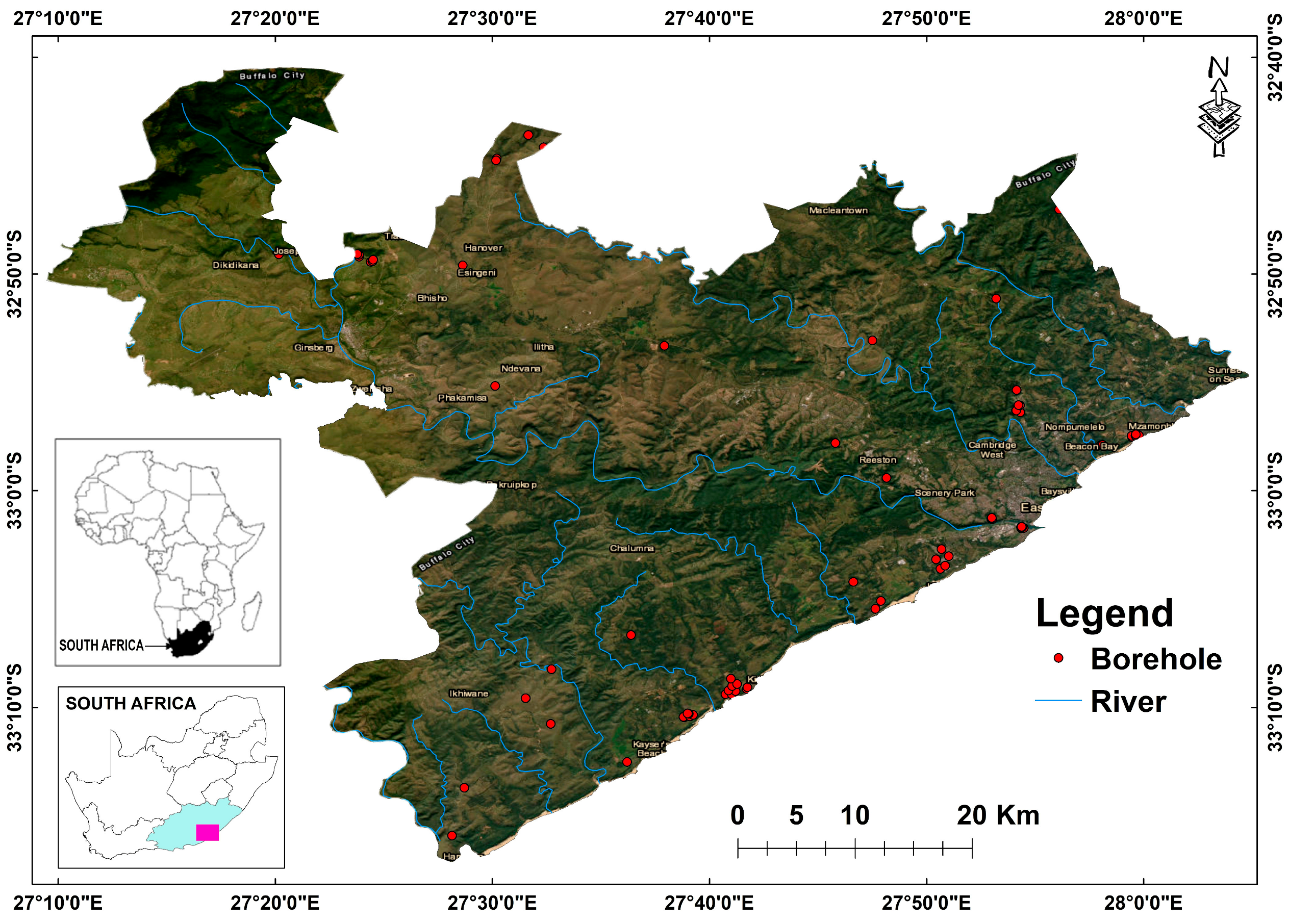
2.1. Study Area
2.2. Data Sources
2.3. Analytical Hierarchy Process (AHP)
2.3.1. Pairwise Comparison Matrix and Weighting of Each Groundwater Controlling Factor
2.3.2. Consistency Ratio (CR) Calculation
2.3.3. Groundwater Potential Zone (GWPZ) Model
2.4. Frequency Ratio (FR)
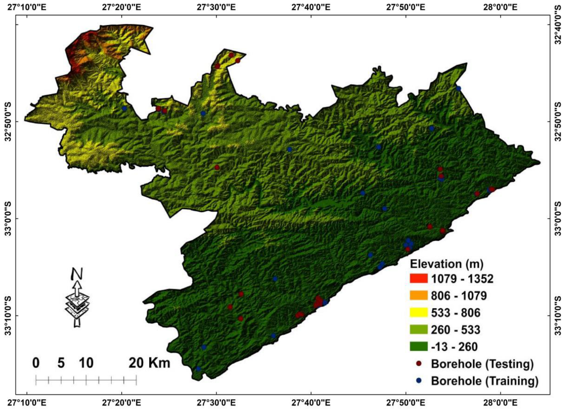
2.5. Borehole Data
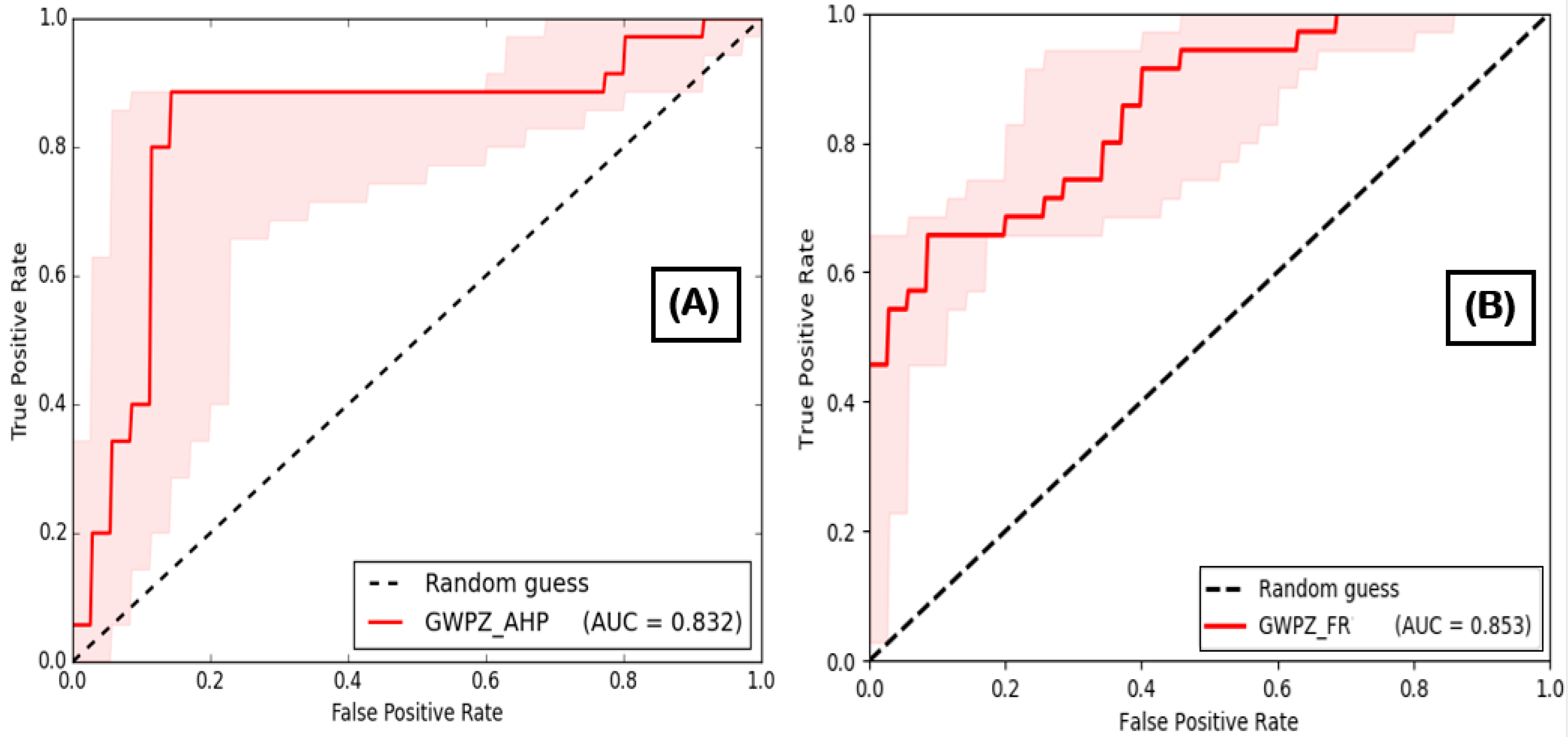
2.6. Validation of AHP and FR Models
3. Results
3.1. Groundwater Controlling Factors
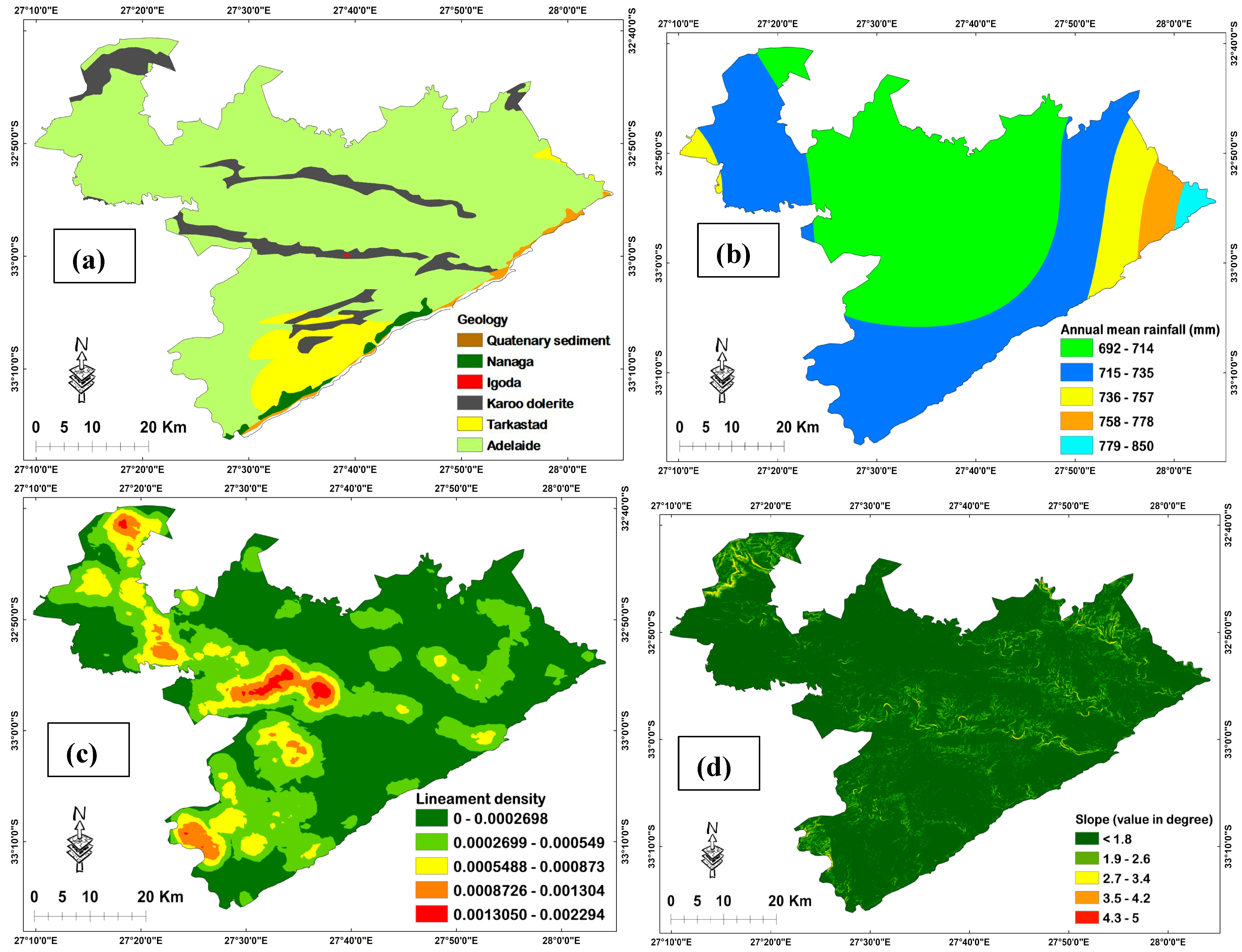
3.1.1. Geology
3.1.2. Rainfall
3.1.3. Lineament Density
3.1.4. Slope
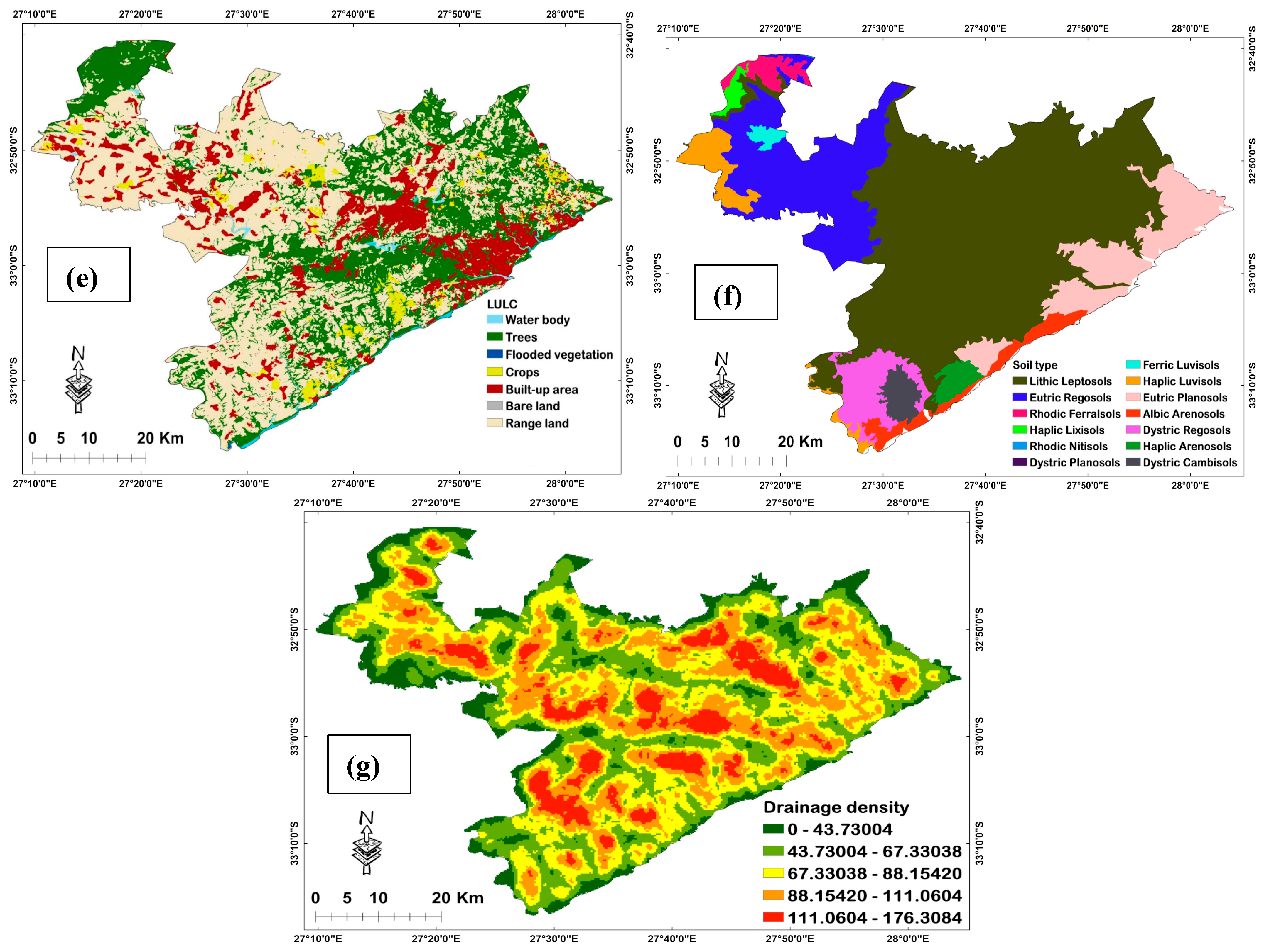
3.1.5. LULC
3.1.6. Soil Type
3.1.7. Drainage Density
3.2. Results of the Models
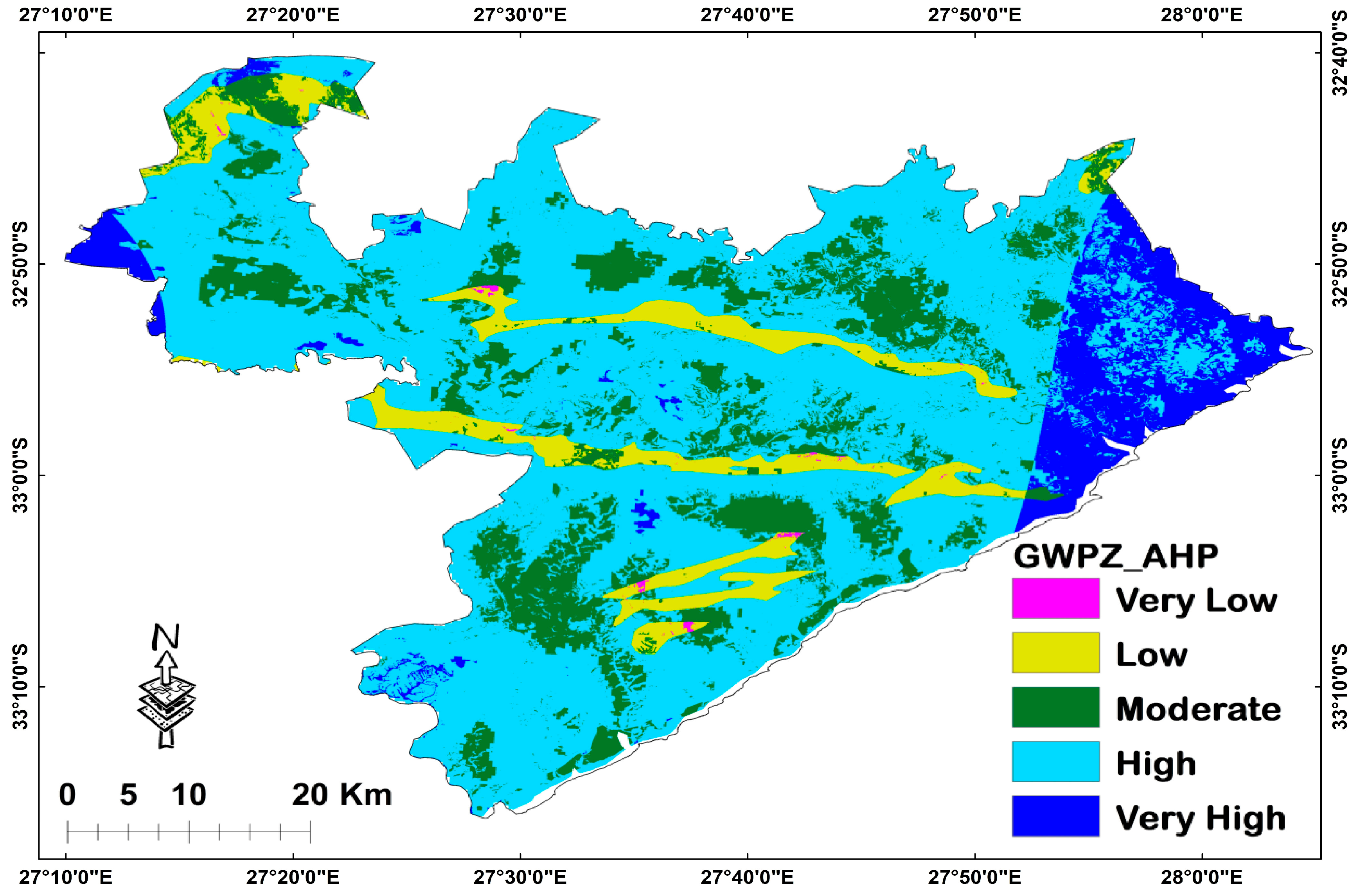
3.2.1. Assessment of Potential Groundwater Recharge Zones Using AHP Model
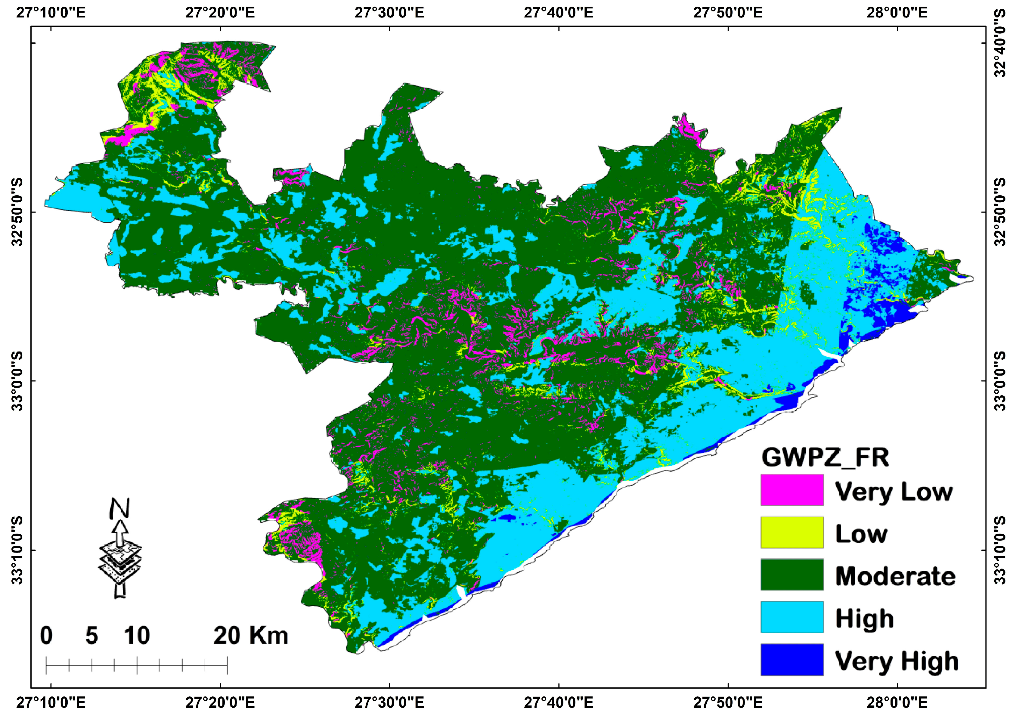
3.2.2. Assessment of Potential Groundwater Recharge Zones Using FR Model
4. Discussion
4.1. Delineation of Potential Groundwater Recharge Zones (GWPZ) Using AHP Model
4.2. Delineation of Potential Groundwater Potential Zones Using FR Model
4.3. Model Validation
5. Conclusions
Author Contributions
Funding
Data Availability Statement
Acknowledgments
Conflicts of Interest
References
- Arabameri, A.; Rezaei, K.; Cerda, A.; Lombardo, L.; Rodrigo-Comino, J. GIS-based groundwater potential mapping in Shahroud plain, Iran. A comparison among statistical (bivariate and multivariate), data mining and MCDM approaches. Sci. Total Environ. 2019, 658, 160–177. [Google Scholar] [CrossRef]
- Mogaji, K.A.; Omobude, O.B. Modeling of geoelectric parameters for assessing groundwater potentiality in a multifaceted geologic terrain, Ipinsa Southwest, Nigeria-A GIS-based GODT approach. NRIAG J. Astron. Geophys. 2017, 6, 434–451. [Google Scholar] [CrossRef]
- Chen, W.; Li, H.; Hou, E.; Wang, S.; Wang, G.; Panahi, M.; Li, T.; Peng, T.; Guo, C.; Niu, C.; et al. GIS-based groundwater potential analysis using novel ensemble weights-of-evidence with logistic regression and functional tree models. Sci. Total Environ. 2018, 634, 853–867. [Google Scholar] [CrossRef]
- Pradhan, R.M.; Guru, B.; Pradhan, B.; Biswal, T.K. Integrated multi-criteria analysis for groundwater potential mapping in Precambrian hard rock terranes (North Gujarat), India. Hydrol. Sci. J. 2021, 6, 961–978. [Google Scholar] [CrossRef]
- Das, S. Comparison among influencing factor, frequency ratio, and analytical hierarchy process techniques for groundwater potential zonation in Vaitarna basin, Maharashtra, India. Groundw. Sustain. Dev. 2019, 8, 617–629. [Google Scholar] [CrossRef]
- Taheri, K.; Taheri, M.; Parise, M. Impact of intensive groundwater exploitation on an unprotected covered arst aquifer: A case study in Kermanshah Province, western Iran. Environ. Earth Sci. 2016, 75, 1221. [Google Scholar] [CrossRef]
- Majidipour, F.; Najafi, S.M.B.; Taheri, K.; Fathollahi, J.; Missimer, T.M. Index-based groundwater sustainability assessment in the socio-economic context: A case study in the Western Iran. Environ. Manag. 2021, 67, 648–666. [Google Scholar] [CrossRef]
- Taheri, K.; Missimer, T.M.; Amini, V.; Bahrami, J.; Omidipour, R. A GIS-expert-based approach for groundwater quality monitoring network design in an alluvial aquifer: A case study and a practical guide. Environ. Monit. Assess. 2020, 192, 1–20. [Google Scholar] [CrossRef]
- Owolabi, S.T.; Madi, K.; Kalumba, A.M. Comparative evaluation of spatio-temporal attributes of precipitation and streamflow in Buffalo and Tyume Catchments, Eastern Cape, South Africa. Environ. Dev. Sustain. 2021, 23, 4236–4251. [Google Scholar] [CrossRef]
- Baudoin, M.A.; Vogel, C.; Nortje, K.; Naik, M. Living with drought in South Africa: Lessons learnt from the recent El Niño drought period. Int. J. Disaster Risk Reduct. 2017, 23, 128–137. [Google Scholar] [CrossRef]
- Nolte, A.; Eley, M.; Schöniger, M.; Gwapedza, D.; Tanner, J.; Mantel, S.K.; Scheihing, K. Hydrological modelling for assessing spatio-temporal groundwater recharge variations in the water-stressed Amathole Water Supply System, Eastern Cape, South Africa: Spatially distributed groundwater recharge from hydrological model. Hydrol. Process. 2021, 35, 14264. [Google Scholar] [CrossRef]
- Mahlalela, P.T.; Blamey, R.C.; Hart, N.C.G.; Reason, C.J.C. Drought in the Eastern Cape region of South Africa and trends in rainfall characteristics. Clim. Dyn. 2020, 55, 2743–2759. [Google Scholar] [CrossRef]
- Muavhi, N.; Thamaga, K.H.; Mutoti, M.I. Mapping groundwater potential zones using relative frequency ratio, analytic hierarchy process and their hybrid models: Case of Nzhelele-Makhado area in South Africa. Geocarto Int. 2022, 37, 6311–6330. [Google Scholar] [CrossRef]
- Das, S.; Gupta, A.; Ghosh, S. Exploring groundwater potential zones using MIF technique in semi-arid region: A case study of Hingoli district, Maharashtra. Spat. Inf. Res. 2017, 25, 749–756. [Google Scholar] [CrossRef]
- Arulbalaji, P.; Padmalal, D.; Sreelash, K. GIS and AHP techniques based delineation of groundwater potential zones: A case study from Southern Western Ghats. India Sci. Rep. 2019, 9, 2082. [Google Scholar] [CrossRef]
- Adesola, G.O.; Gwavava, O.; Liu, K. Hydrological Evaluation of the Groundwater Potential in the Fractured Karoo Aquifer Using Magnetic and Electrical Resistivity Methods: Case Study of the Balfour Formation, Alice, South Africa. Int. J. Geophys. 2023, 2023, 1891759. [Google Scholar] [CrossRef]
- Hasan, M.; Shang, Y.; Akhter, G.; Khan, M. Geophysical investigation of fresh-saline water interface: A case study from South Punjab, Pakistan. Groundwater 2017, 55, 841–856. [Google Scholar] [CrossRef]
- Olatinsu, O.B.; Salawudeen, S.Y. Integrated geophysical investigation of groundwater potential and bedrock structure in Precambrian basement rocks of Ife, southwest Nigeria. Groundw. Sustain. Dev. 2021, 14, 100616. [Google Scholar] [CrossRef]
- McLachlan, P.; Blanchy, G.; Chambers, J.; Sorensen, J.; Uhlemann, S.; Wilkinson, P.; Binley, A. The application of electromagnetic induction methods to reveal the hydrogeological structure of a riparian wetland. Water Resour. Res. 2021, 57, e2020WR029221. [Google Scholar] [CrossRef]
- Pradhan, R.M.; Deshmukh, R.; Chandrasekhar, E.; Balamurugan, G.; Biswal, T.K. Geoelectrical studies for groundwater exploration in fractured rock terrane (Ambaji basin, India). In Proceedings of the Conference of the Arabian Journal of Geosciences, Sousse, Tunisia, 25–28 November 2019; pp. 511–514. [Google Scholar] [CrossRef]
- Sharma, S.P.; Baranwal, V.C. Delineation of groundwater-bearing fracture zones in a hard rock area integrating very low frequency electromagnetic and resistivity data. J. Appl. Geophys. 2005, 2, 155–166. [Google Scholar] [CrossRef]
- Raji, W.O.; Abdulkadir, K.A. Evaluation of groundwater potential of bedrock aquifers in geological sheet 223 Ilorin, Nigeria, using geo-electric sounding. Appl. Water Sci. 2020, 10, 220. [Google Scholar] [CrossRef]
- Akingboye, A.S.; Bery, A.A.; Kayode, J.S.; Ogunyele, A.C.; Adeola, A.O.; Omojola, O.O.; Adesida, A.S. Groundwater-yielding capacity, water-rock interaction, and vulnerability assessment of typical gneissic hydrogeologic units using geoelectrohydraulic method. Acta Geophys. 2023, 71, 697–721. [Google Scholar] [CrossRef]
- Pradhan, R.M.; Singh, A.; Ojha, A.K.; Biswal, T.K. Structural controls on bedrock weathering in crystalline basement terranes and its implications on groundwater resources. Sci. Rep. 2022, 1, 11815. [Google Scholar] [CrossRef] [PubMed]
- Akingboye, A.S.; Bery, A.A.; Kayode, J.S.; Asulewon, A.M.; Bello, R.; Agbasi, O.E. Near-surface crustal architecture and geohydrodynamics of the crystalline basement terrain of Araromi, Akungba-Akoko, SW Nigeria, derived from multi-geophysical methods. Nat. Resour. Res. 2022, 31, 215–236. [Google Scholar] [CrossRef]
- Nampak, H.; Pradhan, B.; Manap, M.A. Application of GIS based data driven evidential belief function model to predict groundwater potential zonation. J. Hydrol. 2014, 513, 283–300. [Google Scholar] [CrossRef]
- Guru, B.; Seshan, K.; Bera, S. Frequency ratio model for groundwater potential mapping and its sustainable management in cold desert, India. J. King Saud. Univ.-Sci. 2017, 29, 333–347. [Google Scholar] [CrossRef]
- Kumar, V.A.; Mondal, N.C.; Ahmed, S. Identification of groundwater potential zones using RS, GIS and AHP techniques: A case study in a part of Deccan Volcanic Province (DVP), Maharashtra, India. J. Indian. Soc. Remote Sens. 2020, 48, 497–511. [Google Scholar] [CrossRef]
- Singh, L.K.; Jha, M.K.; Chowdary, V.M. Assessing the accuracy of GIS-based Multi-Criteria Decision Analysis approaches for mapping groundwater potential. Ecol. Indicat. 2018, 91, 24–37. [Google Scholar] [CrossRef]
- Rahmati, O.; Pourghasemi, H.R.; Melesse, A.M. Application of GIS-based data driven random forest and maximum entropy models for groundwater potential mapping: A case study at Mehran Region, Iran. Catena 2016, 137, 360–372. [Google Scholar] [CrossRef]
- Kim, J.C.; Jung, H.S.; Lee, S. Groundwater productivity potential mapping using frequency ratio and evidential belief function and artificial neural network models: Focus on topographic factors. J. Hydroinformatics 2018, 20, 1436–1451. [Google Scholar] [CrossRef]
- Andualem, T.G.; Demeke, G.G. Groundwater potential assessment using GIS and remote sensing: A case study of Guna tana landscape, upper Blue Nile Basin, Ethiopia. J. Hydrol. Reg. Stud. 2019, 24, 100610–100613. [Google Scholar] [CrossRef]
- Ahirwar, S.; Malik, M.S.; Ahirwar, R.; Shukla, J.P. Identification of suitable sites and structures for artificial groundwater recharge for sustainable groundwater resource development and management. Groundwater Sustain. Develop 2020, 11, 100388. [Google Scholar] [CrossRef]
- Jenifer, M.A.; Jha, M.K. Comparison of analytical hierarchy process, catastrophe and entropy techniques for evaluating groundwater prospect of hard-rock aquifer systems. J. Hydrol. 2017, 548, 605–624. [Google Scholar] [CrossRef]
- Kumar, A.; Krishna, A.P. Assessment off groundwater potential zones in coal mining impacted hard-rock terrain of India by integrating geospatial and analytic hierarchy process (AHP) approach. Geocarto Int. 2018, 33, 105–129. [Google Scholar] [CrossRef]
- Saranya, T.; Saravanan, S. Groundwater potential zone mapping using analytical hierarchy process (AHP) and GIS for Kancheepuram District, Tamilnadu, India. Model. Earth Syst. Environ. 2020, 6, 1105–1122. [Google Scholar] [CrossRef]
- Taheri, K.; Missimer, T.M.; Taheri, M.; Moayedi, H.; Mohseni Pour, F. Critical zone assessments of an alluvial aquifer system using the multi-influencing factor (MIF) and analytical hierarchy process (AHP) models in Western Iran. Nat. Resour. Res. 2020, 29, 1163–1191. [Google Scholar] [CrossRef]
- Chowdary, V.; Chakraborthy, D.; Jeyaram, A.; Murthy, Y.K.; Sharma, J.; Dadhwal, V. Multi-Criteria decision making approach for watershed prioritization using analytic hierarchy process technique and GIS. Water Resour. Manag. 2013, 27, 3555–3571. [Google Scholar] [CrossRef]
- Moghaddam, D.D.; Rezaei, M.; Pourghasemi, H.R.; Pourtaghie, Z.S.; Pradhan, B. Groundwater spring potential mapping using bivariate statistical model and GIS in the Taleghan watershed, Iran. Arab. J. Geosci. 2015, 8, 913–929. [Google Scholar] [CrossRef]
- Das, S.; Pardeshi, S.D. Integration of different influencing factors in GIS to delineate groundwater potential areas using IF and FR techniques: A study of Pravara basin, Maharashtra, India. Appl. Water Sci. 2018, 8, 197. [Google Scholar] [CrossRef]
- Trabelsi, F.; Lee, S.; Khlifi, S.; Arfaoui, A. Frequency ratio model for mapping groundwater potential zones using GIS and remote sensing; Medjerda Watershed Tunisia. In Advances in Science, Technology & Innovation; Springer Publishing: New York, NY, USA, 2019; pp. 341–345. [Google Scholar] [CrossRef]
- Lee, S.; Kim, Y.S.; Oh, H.J. Application of a weights-of-evidence method and GIS to regional groundwater productivity potential mapping. J. Environ. Manag. 2012, 1, 91–105. [Google Scholar] [CrossRef]
- Nejad, S.G.; Falah, F.; Daneshfar, M.; Haghizadeh, A.; Rahmati, O. Delineation of groundwater potential zones using remote sensing and GIS-based data-driven models. Geocarto Int. 2017, 2, 167–187. [Google Scholar]
- Sahoo, S.; Munusamy, S.B.; Dhar, A.; Kar, A.; Ram, P. Appraising the accuracy of multiclass frequency ratio and weights of evidence method for delineation of regional groundwater potential zones in canal command system. Water Resour. Manag. 2017, 14, 4399–4413. [Google Scholar] [CrossRef]
- Rahmati, O.; Kornejady, A.; Samadi, M.; Nobre, A.D.; Melesse, A.M. Development of an automated GIS tool for reproducing the HAND terrain model. Environ. Model. Softw. 2018, 102, 1–12. [Google Scholar] [CrossRef]
- Antonakos, A.K.; Voudouris, K.S.; Lambrakis, N.I. Site selection for drinking-water pumping boreholes using a fuzzy spatial decision support system in the Korinthia prefecture, SE Greece. Hydrogeol. J. 2014, 8, 1763–1776. [Google Scholar] [CrossRef]
- Rahmati, O.; Melesse, A.M. Application of Dempster–Shafer theory, spatial analysis and remote sensing for groundwater potentiality and nitrate pollution analysis in the semi-arid region of Khuzestan, Iran. Sci. Total Environ. 2016, 568, 1110–1123. [Google Scholar] [CrossRef]
- Ozdemir, A. GIS-based groundwater spring potential mapping in the Sultan Mountains (Konya, Turkey) using frequency ratio, weights of evidence and logistic regression methods and their comparison. J. Hydrol. 2011, 411, 290–308. [Google Scholar] [CrossRef]
- Naghibi, S.A.; Pourghasemi, H.R.; Pourtaghi, Z.S.; Rezaei, A. Groundwater qanat potential mapping using frequency ratio and Shannon’s entropy models in the Moghan watershed, Iran. Earth Sci. Inform. 2015, 8, 171–186. [Google Scholar] [CrossRef]
- Golkarian, A.; Naghibi, S.A.; Kalantar, B.; Pradhan, B. Groundwater potential mapping using C5.0, random forest, and multivariate adaptive regression spline models in GIS. Environ. Monit. Assess. 2018, 3, 149. [Google Scholar] [CrossRef]
- Golkarian, A.; Rahmati, O. Use of a maximum entropy model to identify the key factors that influence groundwater availability on the Gonabad Plain. Iran. Env. Earth Sci. 2018, 77, 369. [Google Scholar] [CrossRef]
- Chenini, I.; Mammou, A.B. Groundwater recharge study in arid region: An approach using GIS techniques and numerical modeling. Comput. Geosci. 2010, 6, 801–817. [Google Scholar] [CrossRef]
- Naghibi, S.A.; Pourghasemi, H.R.; Abbaspour, K.A. comparison between ten advanced and soft computing models for groundwater qanat potential assessment in Iran using R and GIS. Theor. Appl. Climatol. 2018, 131, 967–984. [Google Scholar] [CrossRef]
- Saaty, T.L. The Analytic Hierarchy Process: Planning, Priority Setting, Resource Allocation; McGraw: New York, NY, USA, 1980; p. 281. [Google Scholar]
- Nel, J.; Colvin, C.; Le Maitre, D.; Smith, J.; Haines, I. South Africa’s Strategic Water Source Areas (No. CSIR/NRE/ECOS/ER/2013/0031/a); WWF-SA: Cape Town, South Africa, 2013; p. 27. [Google Scholar]
- Department of Water and Sanitation (DWS). Amatole Water Supply System Reconciliation Strategy: Status Report: October 2016; Department of Water and Sanitation (DWS): Pretoria, South Africa, 2016; p. 90.
- Dube, R.A.; Maphosa, B.; Fayemiwo, O.M. Adaptive Climate Change Technologies and Approaches for Local Governments: Water Sector Response; WRC Report No. TT; Water Research Commission: Pretoria, South Africa, 2016; Volume 663, p. 16. [Google Scholar]
- Botai, C.M.; Botai, J.O.; Adeola, A.M.; de Wit, J.P.; Ncongwane, K.P.; Zwane, N.N. Drought risk analysis in the Eastern Cape Province of South Africa: The copula lens. Water 2020, 12, 1938. [Google Scholar] [CrossRef]
- Cobbing, J. Groundwater for Rural Water Supplies in South Africa; Nelson Mandela Metropolitan University: Gqeberha, South Africa; SLR Consulting (Pty) Ltd.: Pretoria, South Africa, 2014. [Google Scholar]
- Cobbing, J.E.; de Wit, M. The Grootfontein aquifer: Governance of a hydro-social system at Nash equilibrium. South. Afr. J. Sci. 2018, 114, 20170230. [Google Scholar] [CrossRef] [PubMed]
- Olivier, D.W.; Xu, Y. Making effective use of groundwater to avoid another water supply crisis in Cape Town, South Africa. Hydrogeol. J. 2019, 27, 823–826. [Google Scholar] [CrossRef]
- Algaydi, B.A.M.; Subyani, A.M.; Hamza, M.H.M.M. Investigation of groundwater potential zones in hard rock Terrain, Wadi Na’man, Saudi Arabia. Groundwater 2019, 57, 940–950. [Google Scholar] [CrossRef]
- Statistic South Africa. Census 2011: Census in Brief; Statistics South Africa: Pretoria, South Africa, 2012.
- Department of Water Affairs and Forestry (DWAF). State-of-Rivers Report: Buffalo River System (River Health Programme); Department of Water Affairs and Forestry: KwaZulu-Natal, South Africa, 2004; Volume 8, p. 102.
- Johnson, M.; van Vuuren, C.; Visser, J.; Cole, D.; de Wickens, H.; Christie, A.; Roberts, D. The Foreland Karoo Basin, South Africa. In African Sedimentary Basins of the World; Selley, R., Ed.; Elsevier: Amsterdam, The Netherlands, 1997; Volume 3, pp. 269–317. [Google Scholar]
- Department of Water Affairs and Forestry (DWAF). Development of a Reconciliation Strategy for the Amatole Bulk Water Supply System; Final Report (No. PWMA 12/R00/00/2608); Department of Water Affairs and Forestry: KwaZulu-Natal, South Africa, 2008; p. 134.
- Hashim, M.; Ahmad, S.; Johari, M.A.M.; Pour, A.B. Automatic lineament extraction in a heavily vegetated region using Landsat Enhanced Thematic Mapper (ETM+) imagery. Adv. Space Res. 2013, 51, 874–890. [Google Scholar] [CrossRef]
- Sener, S.; Sener, E.; Karaguzel, R. Solid waste disposal site selection with GIS and AHP methodology: A case study in Senirkent-Uluborly (Isparta) Basin, Turkey. Environ. Monit. Assess. 2011, 173, 533–554. [Google Scholar] [CrossRef]
- Pourtaghi, Z.S.; Pourghasemi, H.R. GIS-based groundwater spring potential assessment and mapping in the Birjand Township, southern Khorasan Province Iran. Hydrogeology 2014, 22, 643–662. [Google Scholar] [CrossRef]
- Jenks, G.F. The data model concept in statistical mapping. Int. Year Book. Cartogr. 1967, 7, 186–190. [Google Scholar]
- Oh, H.J.; Lee, S. Assessment of ground subsidence using GIS and the weights-of-evidence model. Eng. Geol. 2010, 115, 36–48. [Google Scholar] [CrossRef]
- Jasrotia, A.S.; Kumar, R.; Saraf, A.K. Delineation of groundwater recharge sites using integrated remote sensing and GIS in Jammu district, India. Int. J. Remote Sens. 2007, 28, 5019–5036. [Google Scholar] [CrossRef]
- Stroebel, D.H.; Thiart, C.; de Wit, M. Towards defining a baseline status of scarce groundwater resources in anticipation of hydraulic fracturing in the Eastern Cape Karoo, South Africa: Salinity, aquifer yields and groundwater levels. Geol. Soc. Lond. Spec. Publ. 2019, 479, 129–145. [Google Scholar] [CrossRef]
- Barlow, P.M.; Leake, S.A. Streamflow Depletion by Wells: Understanding and Managing the Effects of Groundwater Pumping on Streamflow; US Geological Survey: Reston, VA, USA, 2012; Volume 1376, 84p. [CrossRef]
- Xu, Y.; Lin, L.; Jia, H. Groundwater Flow Conceptualization and Storage Determination of the Table Mountain Group (TMG) Aquifers; WRC Report, (1419/1); Water Research Commission: Pretoria, South Africa, 2009; p. 9. [Google Scholar]
- Kindie, A.T.; Enku, T.; Moges, M.A.; Geremew, B.S.; Atinkut, H.B. Spatial analysis of groundwater potential using GIS based multi criteria decision analysis method in Lake Tana Basin, Ethiopia. In Proceedings of the Advances of Science and Technology: 6th EAI International Conference, ICAST 2018, Bahir Dar, Ethiopia, 5–7 October 2018; Springer International Publishing: Berlin/Heidelberg, Germany, 2019; Volume 6, pp. 439–456. [Google Scholar] [CrossRef]
- Masoud, A.M.; Pham, Q.B.; Alezabawy, A.K.; El-Magd, S.A.A. Efficiency of geospatial technology and multi-criteria decision analysis for groundwater potential mapping in a Semi-Arid region. Water 2022, 14, 882. [Google Scholar] [CrossRef]
- Dar, T.; Rai, N.; Bhat, A. Delineation of potential groundwater recharge zones using analytical hierarchy process (AHP). Geol. Ecol. Landsc. 2021, 5, 292–307. [Google Scholar] [CrossRef]
- Hagos, Y.G.; Andualem, T.G. Geospatial and multi-criteria decision approach of groundwater potential zone identification in Cuma sub-basin. Southern Ethiopia. Heliyon 2021, 7, e07963. [Google Scholar] [CrossRef] [PubMed]
- Rajesh, J.; Pande, C.B.; Kadam, S.A.; Gorantiwar, S.D.; Shinde, M.G. Exploration of groundwater potential zones using analytical hierarchical process (AHP) approach in the Godavari River basin of Maharashtra in India. Appl. Water Sci. 2021, 11, 182. [Google Scholar] [CrossRef]
- Owolabi, S.T.; Madi, K.; Kalumba, A.M.; Orimoloye, I.R. A groundwater potential zone mapping approach for semi-arid environments using remote sensing (RS), geographic information system (GIS), and analytical hierarchical process (AHP) techniques: A case study of Buffalo catchment, Eastern Cape, South Africa. Arab. J. Geosci. 2020, 13, 1–17. [Google Scholar] [CrossRef]
- Chevalier, L.; Goedhart, M.; Woodford, A.C. The Influence of Dolerite Sill and Ring Complexes on the Occurrence of Groundwater in Karoo Fractured Aquifers: A Morpho-Tectonic Approach; WRC Report No. 937/1/01; Water Research Commission: Pretoria, South Africa, 2001; p. 165. [Google Scholar]
- Nisar, U.B.; Ehsan, S.A.; Farooq, M.; Pant, R.R.; Khan, N.G.; Qaiser, F.U.R.; Butt, F.M. Integrated Geoelectrical and Geological Investigation of a Quaternary Paleo-Depositional Environment in the Haripur Basin, Northern Pakistan: Implications for Groundwater System. Geofluids 2023, 13, 1057457. [Google Scholar] [CrossRef]
- Murray, R.; Cobbing, J.; Woodford, A.; Ravenscroft, L.; Chevallier, L. Groundwater Research Needs in the Eastern Karoo Basin of South Africa; Water Research Commission: Pretoria, South Africa, 2006; p. 52. [Google Scholar]
- Abdekareem, M.; Abdalla, F.; Al-Arifi, N.; Bamousa, A.O.; El-Baz, F. Using remote sensing and GIS-based frequency ratio technique for revealing groundwater prospective areas at Wadi Al Hamdh watershed, Saudi Arabia. Water 2023, 15, 1154. [Google Scholar] [CrossRef]
- Tolche, A.D. Groundwater potential mapping using geospatial techniques: A case study of Dhungeta-Ramis sub-basin, Ethiopia. Geol. Ecol. Landsc. 2021, 5, 65–80. [Google Scholar] [CrossRef]
- Nachtergaele, F.; van Velthuizen, H.; Verelst, L.; Wiberg, D.; Henry, M.; Chiozza, F.; Yigini, Y.; Aksoy, E.; Batjes, N.; Boateng, E.; et al. Harmonized World Soil Database; version 2.0; Food and Agriculture Organization of the United Nations: Rome, Italy, 2023; p. 69.
- Pradhan, B. Groundwater potential zonation for basaltic watersheds using satellite remote sensing data and GIS techniques. Cent. Eur. J. Geosci. 2009, 1, 120–129. [Google Scholar] [CrossRef]
- Fawcett, T. An introduction to ROC analysis. Pattern Recog Lett. 2006, 27, 861–874. [Google Scholar] [CrossRef]


| Matrix | Rainfall | Geology | Slope | Drainage Density | LULC | Lineament Density | Soil | Normalized Principal Eigenvector | |
|---|---|---|---|---|---|---|---|---|---|
| 1 | 2 | 3 | 4 | 5 | 6 | 7 | |||
| Rainfall | 1 | 1 | 3 | 3 | 5 | 5 | 5 | 7 | 38.18% |
| Geology | 2 | 1/3 | 1 | 3 | 3 | 7 | 4 | 5 | 25.01% |
| Slope | 3 | 1/3 | 1/3 | 1 | 1 | 3 | 3 | 3 | 12.11% |
| Drainage density | 4 | 1/5 | 1/3 | 1 | 1 | 1 | 2 | 3 | 9.09% |
| LULC | 5 | 1/5 | 1/7 | 1/3 | 1 | 1 | 1 | 1 | 5.43% |
| Lineament density | 6 | 1/5 | 1/4 | 1/3 | 1/2 | 1 | 1 | 3 | 6.25% |
| Soil | 7 | 1/7 | 1/5 | 1/3 | 1/3 | 1 | 1/3 | 1 | 3.94% |
| CR = 4.5% | |||||||||
| Factor | Sub-Class | Rank | Factor | Sub-Class | Rank |
|---|---|---|---|---|---|
| Geology | Quaternary sediment | 5 | Soil Type | Albic Arenosols | 3 |
| Nanaga | 4 | Haplic Arenosols | 3 | ||
| Igoda | 5 | Dystric Cambisols | 5 | ||
| Karoo dolerite | 3 | Rhodic Ferralsols | 3 | ||
| Tarkastad | 5 | Lithic Leptosols | 2 | ||
| Adelaide | 5 | Ferric Luvisols | 4 | ||
| Rainfall (mm) | 692–714 | 4 | Haplic Luvisols | 4 | |
| 715–735 | 4 | Haplic Lixisols | 5 | ||
| 736–757 | 4 | Rhodic Nitisols | 3 | ||
| 758–778 | 5 | Dystric Planosols | 2 | ||
| 779–850 | 5 | Eutric Planosols | 2 | ||
| Lineament Density | 0–0.0002698 | 1 | Dystric Regosols | 3 | |
| 0.0002699–0.000549 | 2 | Eutric Regosols | 3 | ||
| 0.0005488–0.000873 | 3 | Drainage Density | 0–43.73004 | 5 | |
| 0.0008726–0.001304 | 4 | 43.73005–67.33038 | 4 | ||
| 0.0013050–0.002294 | 5 | 67.33039–88.15420 | 3 | ||
| Slope (°) | <1.8 | 5 | 88.15421–111.0604 | 2 | |
| 1.9–2.6 | 4 | 111.0605–176.3084 | 1 | ||
| 2.7–3.4 | 3 | ||||
| 3.5–4.2 | 2 | ||||
| 4.3–5.0 | 1 | ||||
| LULC | Water body | 5 | |||
| Trees | 3 | ||||
| Flooded vegetation | 5 | ||||
| Crops | 3 | ||||
| Built-up area | 1 | ||||
| Bare land | 2 | ||||
| Rangeland | 1 |
| Soil Types | Description |
|---|---|
| Arenosols (Albic and Haplic) | Sandy loam soils with very weak or no soil development. |
| Luvisols (Ferric and Haplic) | Brown/reddish brown with clay to silty clay texture, moderately well to well-drained weathered soils. |
| Regosols (Eutric and Dystric) | Sandy loam to loam, excessively drained soils with no or little soil development. |
| Nitisols (Rhodic) | Dark red or dusty red clayey soils having a pronounced shiny, nut-shaped structure, silty clay to clay well-drained soil. |
| Lixisols (Haplic) | Red-yellow soils with subsurface accumulation of low activity clays and high base saturation, low activity clays, and a moderate to high base saturation level. |
| Leptosols (Lithic) | Clay loam to clay, very shallow soils over a hard rock or in unconsolidated very gravelly material, soil with no or little soil developments. |
| Cambisols (Dystric) | Silty clay moderately to deep and well-drained soils, weakly to moderately developed soils. |
| Planosols (Eutric and Dystric) | Wet soils with a light-colored, temporarily water-saturated topsoil on a low permeable subsoil, soil with low structure stability. |
| Ferralsols (Rhodic) | Deep, strongly weathered, yellow or red soils with a physically stable but chemically poor subsoil, clay assemblage dominated by a low activity of clays. |
| Factor | Subclasses | No of Pixel | % of Subclass | No of BH | % of BH | FR |
|---|---|---|---|---|---|---|
| Geology | Adelaide | 2,288,646 | 81.42 | 27 | 58.70 | 0.72 |
| Karoo dolerite | 263,570 | 9.38 | 5 | 10.87 | 1.16 | |
| Tarkastad | 196,420 | 6.99 | 6 | 13.04 | 1.87 | |
| Quaternary sediment | 26,105 | 0.93 | 7 | 15.22 | 16.38 | |
| Igoda | 367 | 0.01 | 0 | 0 | 0.00 | |
| Nanaga | 35,689 | 1.27 | 1 | 2.17 | 1.71 | |
| Rainfall (mm) | 692–714 | 1,373,343 | 48.50 | 8 | 17.39 | 0.36 |
| 715–735 | 1,151,170 | 40.65 | 23 | 50.00 | 1.23 | |
| 736–757 | 202,583 | 7.15 | 9 | 19.57 | 2.73 | |
| 758–778 | 76,136 | 2.69 | 6 | 13.04 | 4.85 | |
| 779–850 | 28,436 | 1.00 | 0 | 0 | 0.00 | |
| Lineament Density | 0–0.0002698 | 1,541,250 | 54.41 | 29 | 63.04 | 1.16 |
| 0.0002699–0.0005487 | 882,092 | 31.13 | 11 | 23.91 | 0.77 | |
| 0.0005488–0.0008725 | 291,509 | 10.29 | 6 | 13.04 | 1.27 | |
| 0.0008726–0.001304 | 98,378 | 3.47 | 0 | 0 | 0.00 | |
| 0.001305–0.002294 | 19,947 | 0.70 | 0 | 0 | 0.00 | |
| Slope (°) | < 1.8 | 2,613,290 | 91.075 | 46 | 100 | 1.10 |
| 1.9–2.6 | 238,781 | 8.322 | 0 | 0 | 0.00 | |
| 2.7–3.4 | 15,731 | 0.548 | 0 | 0 | 0.00 | |
| 3.5–4.2 | 1495 | 0.052 | 0 | 0 | 0.00 | |
| 4.3–5.0 | 72 | 0.003 | 0 | 0 | 0.00 | |
| LULC | Water body | 25,859 | 0.914 | 0 | 0 | 0.00 |
| Trees | 869,814 | 30.709 | 12 | 26.09 | 0.85 | |
| Flooded vegetation | 1095 | 0.039 | 0 | 0 | 0.00 | |
| Crops | 104,942 | 3.707 | 4 | 8.70 | 2.35 | |
| Built-up area | 419,299 | 14.800 | 19 | 41.30 | 2.79 | |
| Bare land | 9455 | 0.333 | 0 | 0 | 0.00 | |
| Rangeland | 1,402,679 | 49.498 | 11 | 23.91 | 0.48 | |
| Soil Type | Albic Arenosols | 72,443 | 2.570 | 7 | 15.22 | 5.92 |
| Haplic Arenosols | 36,374 | 1.290 | 4 | 8.70 | 6.74 | |
| Dystric Cambisols | 46,054 | 1.634 | 0 | 0 | 0.00 | |
| Rhodic Ferralsols | 42,890 | 1.522 | 0 | 0 | 0.00 | |
| Lithic Leptosols | 1,626,650 | 57.708 | 13 | 28.00 | 0.49 | |
| Ferric Luvisols | 16,996 | 0.603 | 0 | 0 | 0.00 | |
| Haplic Luvisols | 85,552 | 3.035 | 0 | 0 | 0.00 | |
| Haplic Lixisols | 18,028 | 0.640 | 0 | 0 | 0.00 | |
| Rhodic Nitisols | 281 | 0.010 | 0 | 0 | 0.00 | |
| Dystric Planosols | 730 | 0.026 | 0 | 0 | 0.00 | |
| Eutric Planosols | 283,950 | 10.074 | 15 | 32.61 | 3.24 | |
| Dystric Regosols | 119,424 | 4.237 | 2 | 4.35 | 1.03 | |
| Eutric Regosols | 469,401 | 16.653 | 5 | 10.87 | 0.65 | |
| Drainage Density | 0–43.73004 | 308,136 | 10.953 | 4 | 8.70 | 0.79 |
| 43.73005–67.33038 | 727,521 | 25.860 | 18 | 39.13 | 1.51 | |
| 67.33039–88.1542 | 825,658 | 29.348 | 16 | 34.78 | 1.19 | |
| 88.15421–111.0604 | 645,179 | 22.933 | 4 | 8.70 | 0.38 | |
| 111.0605–176.3084 | 306,797 | 10.905 | 4 | 8.70 | 0.80 |
| AHP Model | FR Model | |||||
|---|---|---|---|---|---|---|
| Range | Area (km2) | Area (%) | Range | Area (km2) | Area (%) | |
| Very Low | 257.46–301.50 | 32.33 | 0.13 | 23.35–81.23 | 1012.76 | 4.04 |
| Low | 301.50–345.54 | 1954.31 | 7.80 | 81.23–215.51 | 1218.18 | 4.86 |
| Moderate | 345.54–389.59 | 4412.02 | 17.60 | 215.51–366.00 | 15,610.86 | 62.28 |
| High | 389.59–433.63 | 16,437.17 | 65.57 | 366.00–442.40 | 6787.63 | 27.08 |
| Very High | 433.63–477.67 | 2230.52 | 8.90 | 442.40–613.73 | 436.91 | 1.74 |
Disclaimer/Publisher’s Note: The statements, opinions and data contained in all publications are solely those of the individual author(s) and contributor(s) and not of MDPI and/or the editor(s). MDPI and/or the editor(s) disclaim responsibility for any injury to people or property resulting from any ideas, methods, instructions or products referred to in the content. |
© 2023 by the authors. Licensee MDPI, Basel, Switzerland. This article is an open access article distributed under the terms and conditions of the Creative Commons Attribution (CC BY) license (https://creativecommons.org/licenses/by/4.0/).
Share and Cite
Adesola, G.O.; Thamaga, K.H.; Gwavava, O.; Pharoe, B.K. Groundwater Potential Zones Assessment Using Geospatial Models in Semi-Arid Areas of South Africa. Land 2023, 12, 1877. https://doi.org/10.3390/land12101877
Adesola GO, Thamaga KH, Gwavava O, Pharoe BK. Groundwater Potential Zones Assessment Using Geospatial Models in Semi-Arid Areas of South Africa. Land. 2023; 12(10):1877. https://doi.org/10.3390/land12101877
Chicago/Turabian StyleAdesola, Gbenga Olamide, Kgabo Humphrey Thamaga, Oswald Gwavava, and Benedict Kinshasa Pharoe. 2023. "Groundwater Potential Zones Assessment Using Geospatial Models in Semi-Arid Areas of South Africa" Land 12, no. 10: 1877. https://doi.org/10.3390/land12101877
APA StyleAdesola, G. O., Thamaga, K. H., Gwavava, O., & Pharoe, B. K. (2023). Groundwater Potential Zones Assessment Using Geospatial Models in Semi-Arid Areas of South Africa. Land, 12(10), 1877. https://doi.org/10.3390/land12101877