

U-Net-LSTM: Time Series-Enhanced Lake Boundary Prediction Model

 ,
,  , ,
, ,  , and
, and 
Abstract
:1. Introduction
2. Dataset
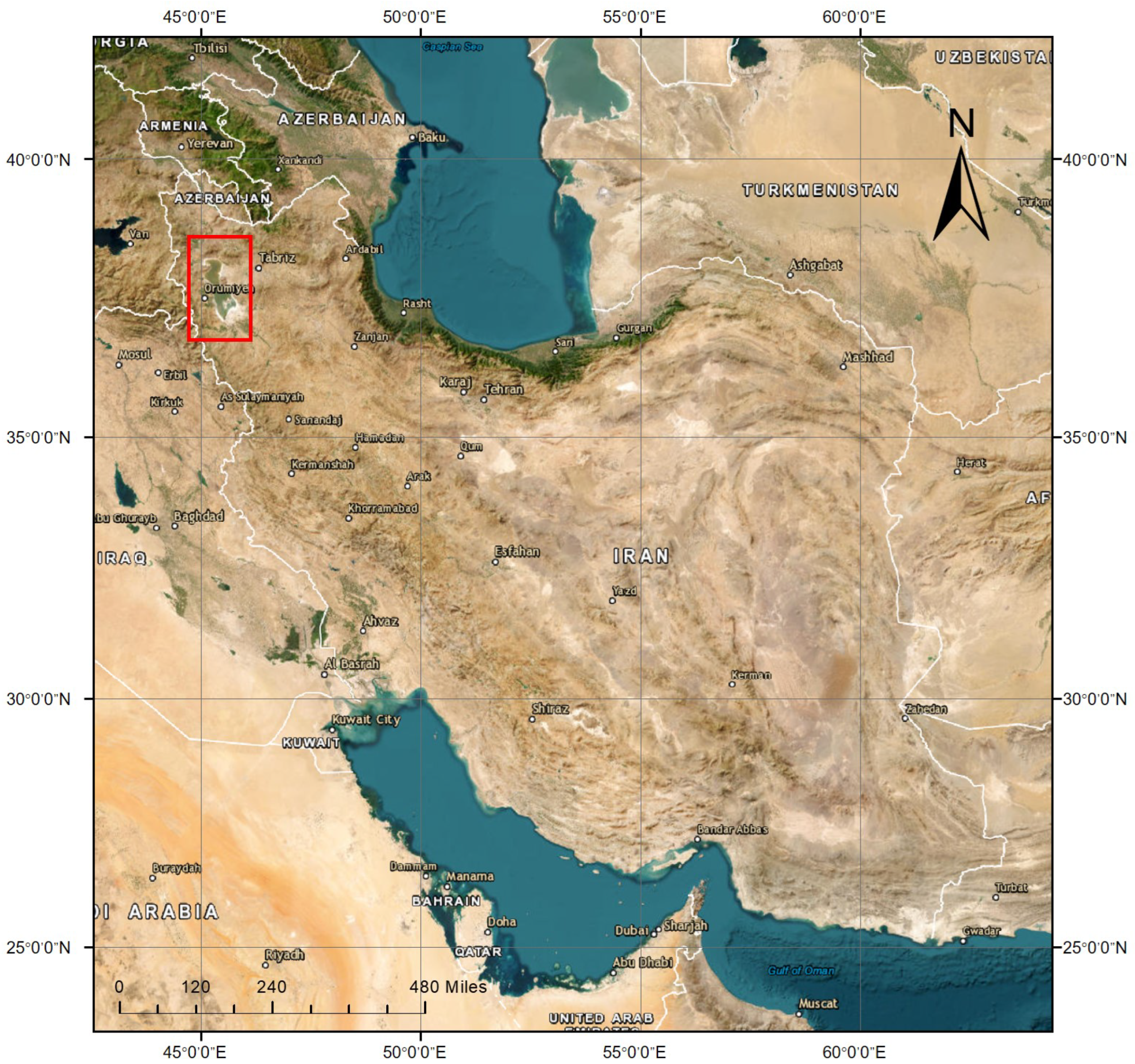
2.1. Data Source
2.2. Data Preprocessing
2.2.1. Image Segmentation
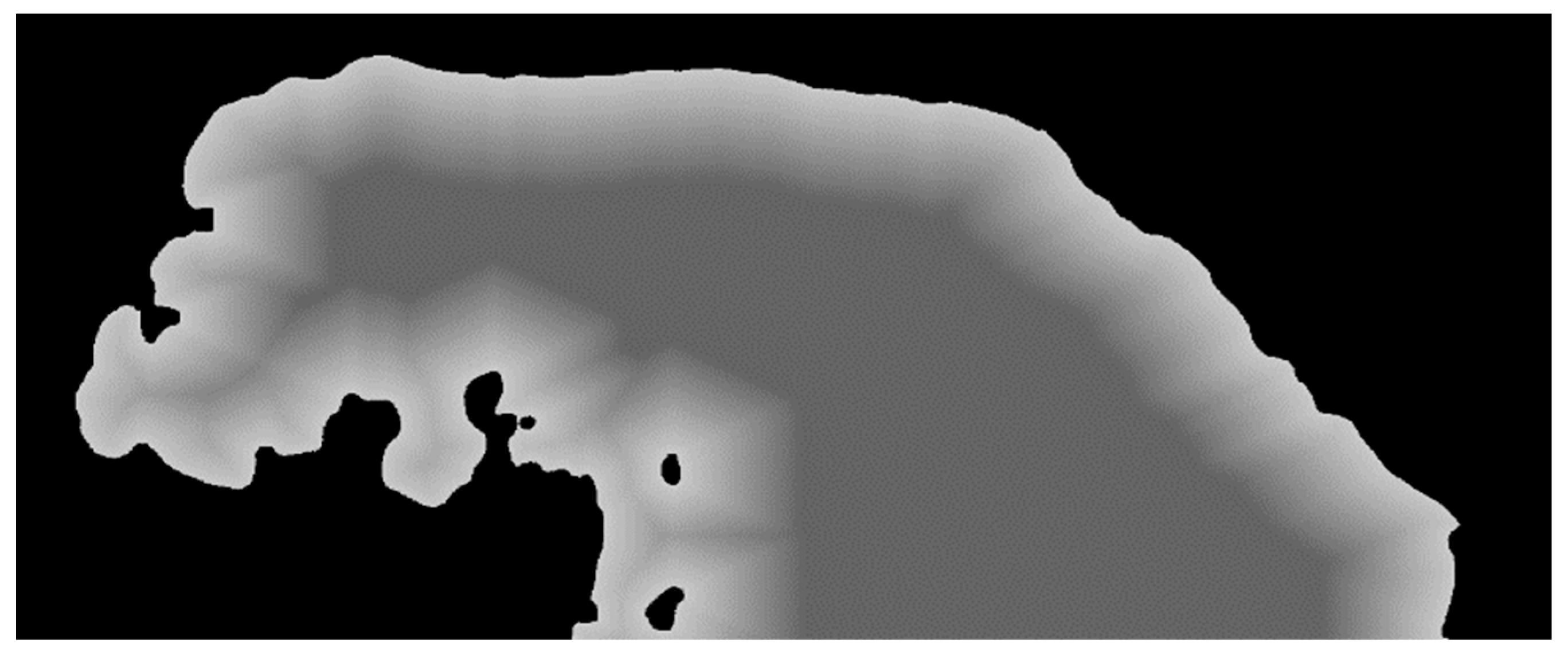
2.2.2. Image Grayscale Gradient Filling
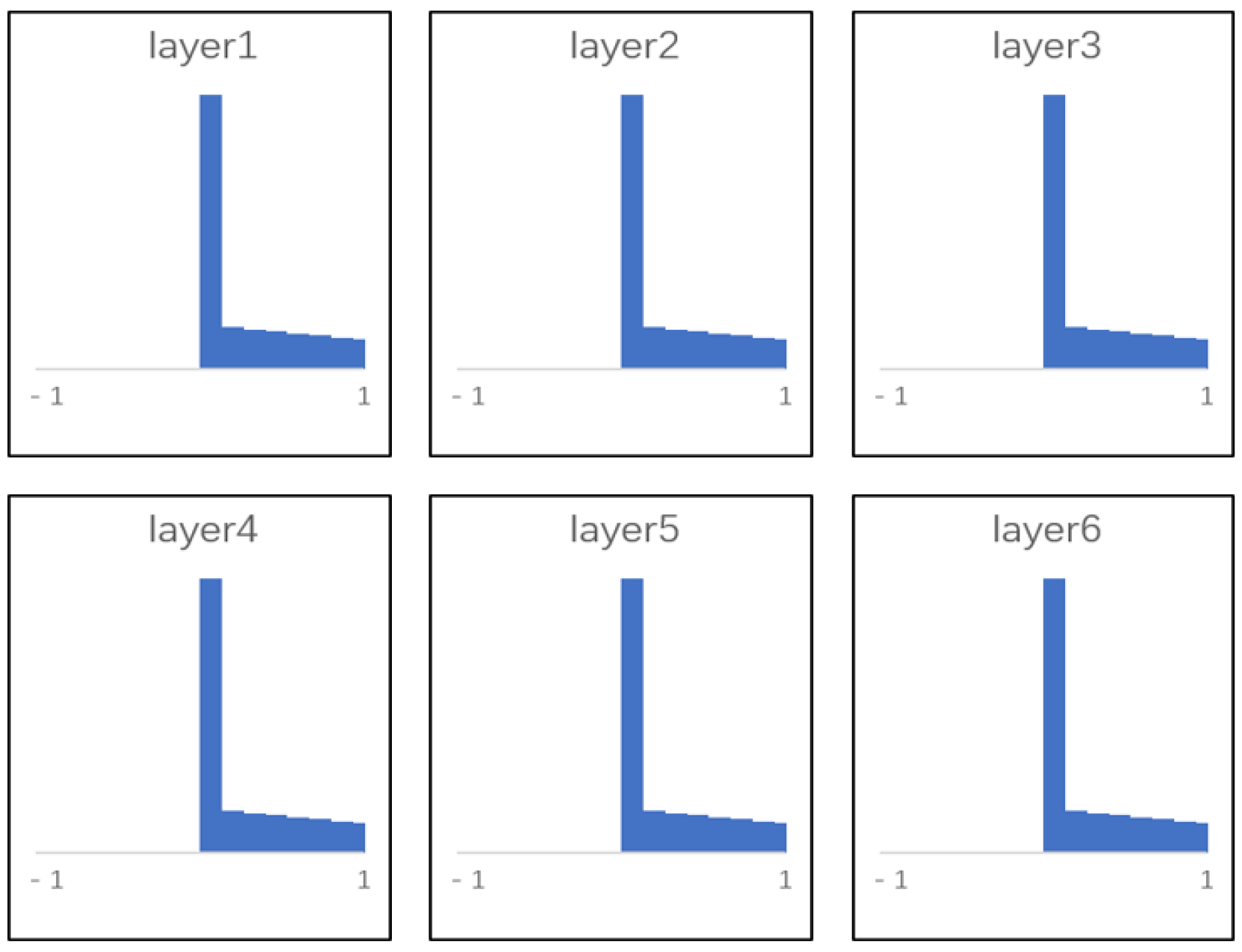
2.2.3. Filtering
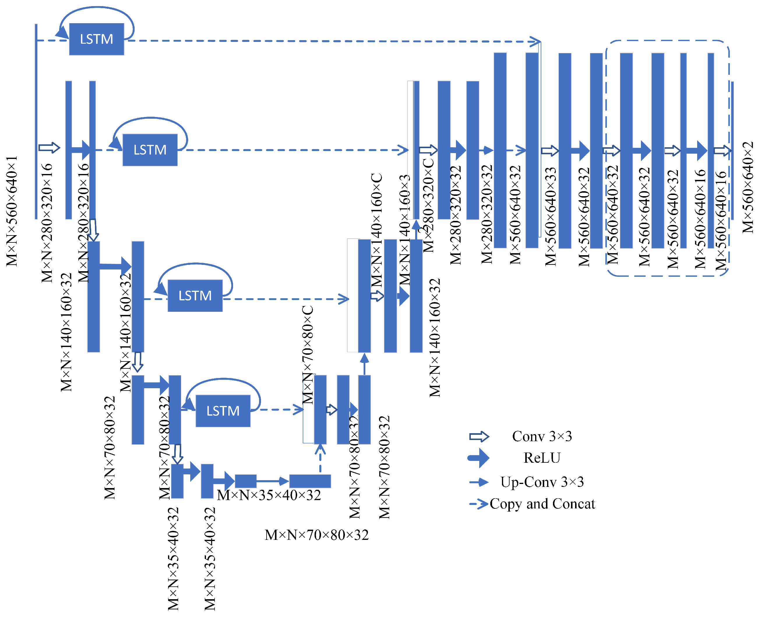
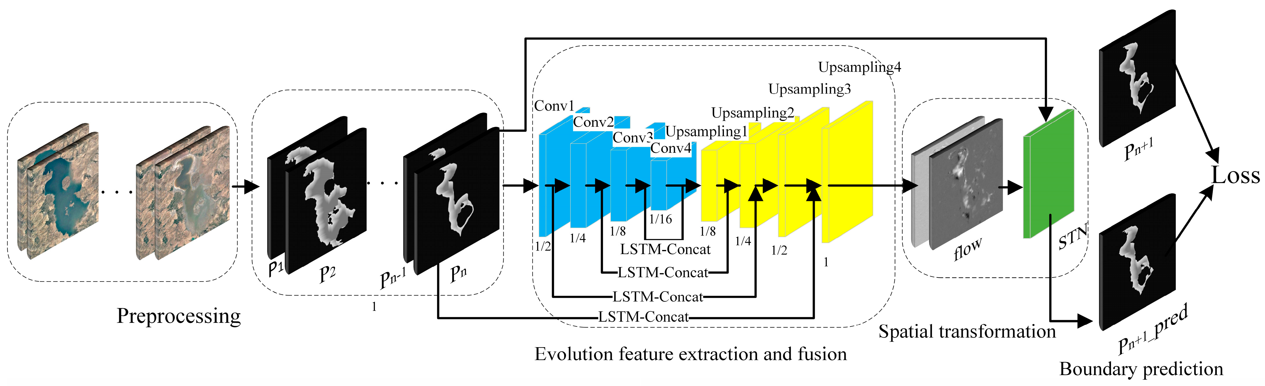
3. Method
3.1. Evolutionary Feature Extraction and Fusion Module
| Algorithm 1: BN algorithm |
| Input: Sample values of a mini-batch: |
| BN layer parameters to be learned: β, γ. |
| Output: . |
| Calculate the sample mean according to Equation (3); |
| Calculate the sample variance according to Equation (4); |
| The sample values are normalized according to Equation (5); |
| γ and β are introduced to translate and scale the sample values, and the sample values are updated according to Equation (6) during backpropagation. |
3.2. Space Transformation Module
3.3. Loss Function
- (1)
- Similarity loss is shown in Equation (8):
- (2)
- Term of penalty is shown in Equation (9):
4. Experiment and Results
4.1. Experiment Setting
4.2. Evaluating Indicators
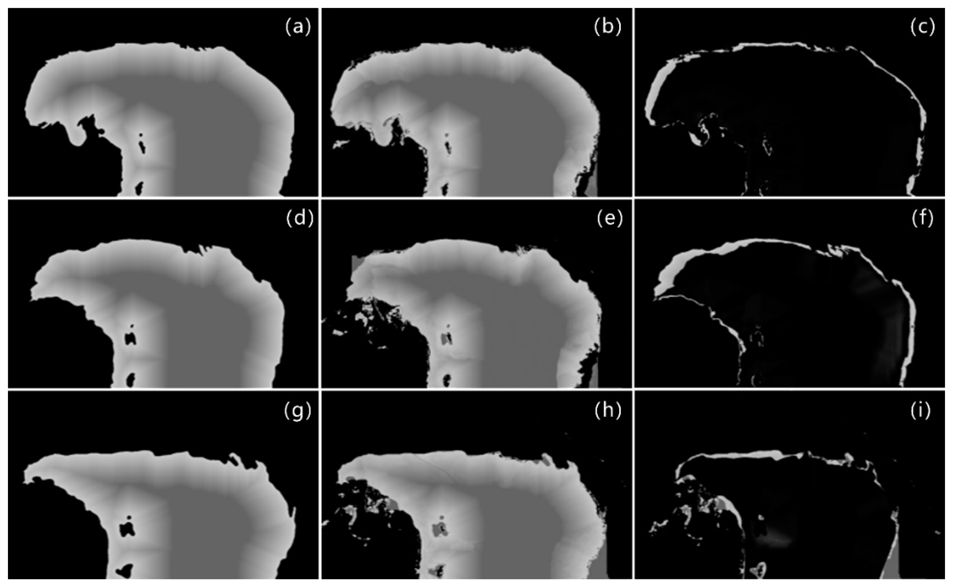
4.3. LSTM Effectiveness Analysis in Experiments 1 and 2
4.3.1. Experiment 1
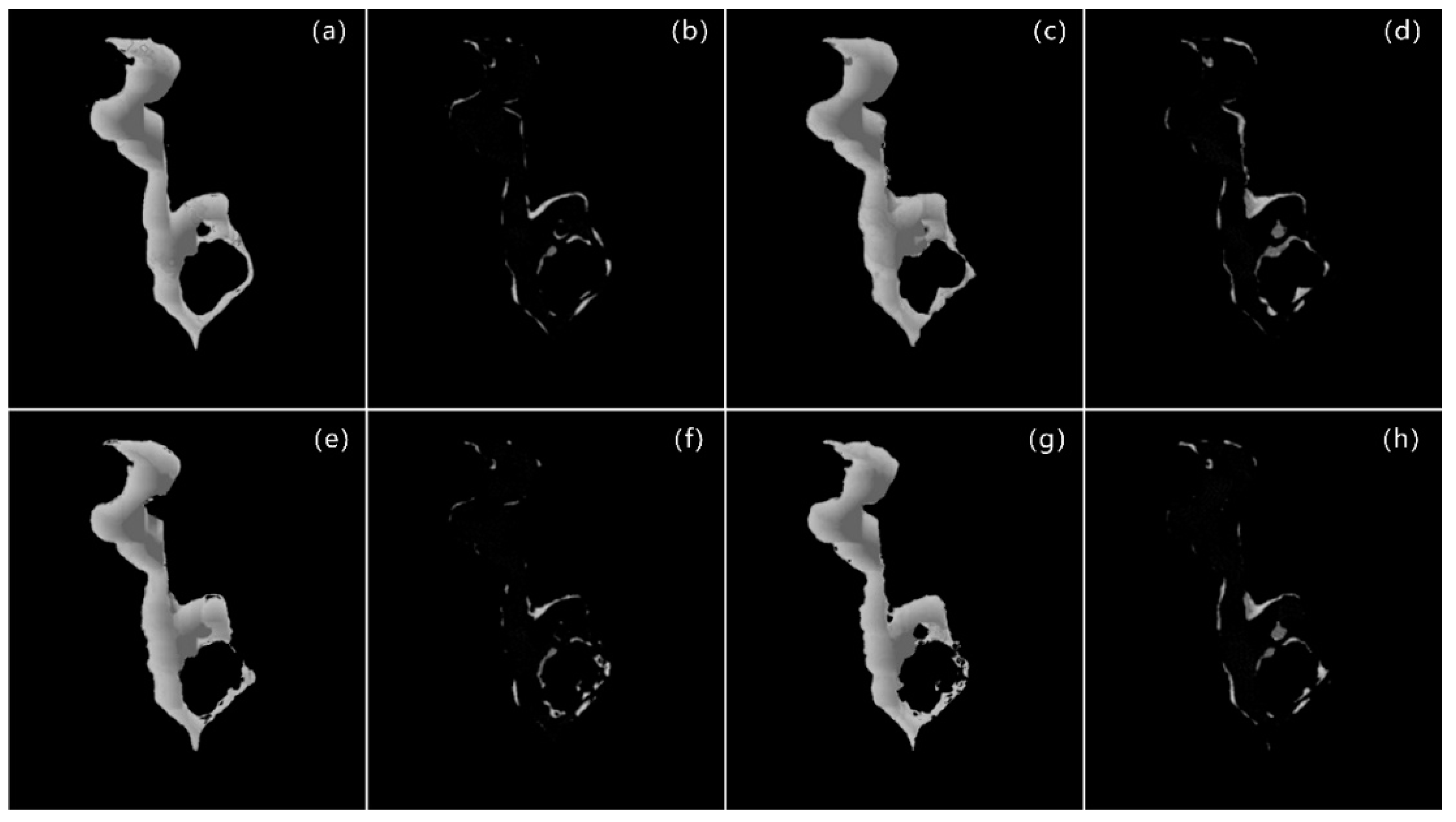
4.3.2. Experiment 2
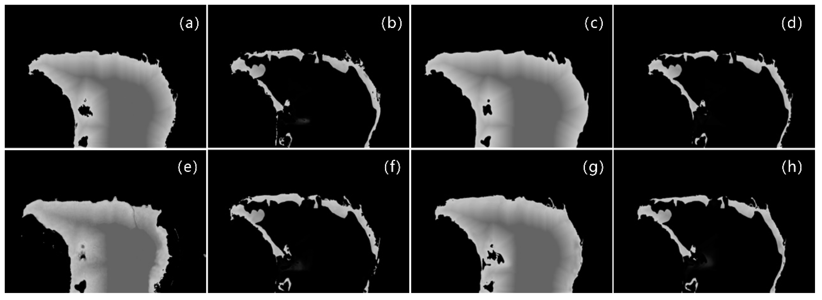
4.4. Time Series Length and Sample Number Analysis
4.4.1. Experiment 3
4.4.2. Experiment 4
5. Discussion
6. Conclusions
Author Contributions
Funding
Data Availability Statement
Conflicts of Interest
References
- Alam, A.; Bhat, M.S.; Maheen, M. Using Landsat satellite data for assessing the land use and land cover change in Kashmir valley. GeoJournal 2020, 85, 1529–1543. [Google Scholar] [CrossRef]
- Arsanjani, J.J. Characterizing, monitoring, and simulating land cover dynamics using GlobeLand30: A case study from 2000 to 2030. J. Environ. Manag. 2018, 214, 66–75. [Google Scholar] [CrossRef] [PubMed]
- Zhang, X.; Han, L.; Han, L.; Zhu, L. How well do deep learning-based methods for land cover classification and object detection perform on high resolution remote sensing imagery? Remote Sens. 2020, 12, 417. [Google Scholar] [CrossRef]
- Qiao, B.; Zhu, L.; Yang, R. Temporal-spatial differences in lake water storage changes and their links to climate change throughout the Tibetan Plateau. Remote Sens. Environ. 2019, 222, 232–243. [Google Scholar] [CrossRef]
- Zhang, G.; Yao, T.; Chen, W.; Zheng, G.; Shum, C.; Yang, K.; Piao, S.; Sheng, Y.; Yi, S.; Li, J. Regional differences of lake evolution across China during 1960s–2015 and its natural and anthropogenic causes. Remote Sens. Environ. 2019, 221, 386–404. [Google Scholar] [CrossRef]
- Hui, F.; Xu, B.; Huang, H.; Yu, Q.; Gong, P. Modelling spatial-temporal change of Poyang Lake using multitemporal Landsat imagery. Int. J. Remote Sens. 2008, 29, 5767–5784. [Google Scholar] [CrossRef]
- Pooja, M.; Thomas, S.; Udayasurya, U.; Praveej, P.; Minu, S. Assessment of Soil Erosion in Karamana Watershed by RUSLE Model Using Remote Sensing and GIS. In Innovative Trends in Hydrological and Environmental Systems: Select Proceedings of ITHES 2021; Springer: Berlin/Heidelberg, Germany, 2022; p. 219. [Google Scholar]
- Wan, W.; Xiao, P.; Feng, X.; Li, H.; Ma, R.; Duan, H.; Zhao, L. Monitoring lake changes of Qinghai-Tibetan Plateau over the past 30 years using satellite remote sensing data. Chin. Sci. Bull. 2014, 59, 1021–1035. [Google Scholar] [CrossRef]
- Symeonakis, E. Modelling land cover change in a Mediterranean environment using Random Forests and a multi-layer neural network model. In Proceedings of the 2016 IEEE International Geoscience and Remote Sensing Symposium (IGARSS), Beijing, China, 10–15 July 2016; pp. 5464–5466. [Google Scholar]
- Zhang, C.; Wei, S.; Ji, S.; Lu, M. Detecting large-scale urban land cover changes from very high resolution remote sensing images using CNN-based classification. ISPRS Int. J. Geo-Inf. 2019, 8, 189. [Google Scholar] [CrossRef]
- Chowdhury, M.; Hasan, M.E.; Abdullah-Al-Mamun, M. Land use/land cover change assessment of Halda watershed using remote sensing and GIS. Egypt. J. Remote Sens. Space Sci. 2020, 23, 63–75. [Google Scholar] [CrossRef]
- Talukdar, S.; Singha, P.; Mahato, S.; Pal, S.; Liou, Y.-A.; Rahman, A. Land-use land-cover classification by machine learning classifiers for satellite observations—A review. Remote Sens. 2020, 12, 1135. [Google Scholar] [CrossRef]
- Wang, W.; Chen, Y.; Ghamisi, P. Transferring CNN with adaptive learning for remote sensing scene classification. IEEE Trans. Geosci. Remote Sens. 2022, 60, 5533918. [Google Scholar] [CrossRef]
- Zhao, Z.; Li, J.; Luo, Z.; Li, J.; Chen, C. Remote sensing image scene classification based on an enhanced attention module. IEEE Geosci. Remote Sens. Lett. 2020, 18, 1926–1930. [Google Scholar] [CrossRef]
- Liu, F.; Jiao, L.; Tang, X.; Yang, S.; Ma, W.; Hou, B. Local restricted convolutional neural network for change detection in polarimetric SAR images. IEEE Trans. Neural Netw. Learn. Syst. 2018, 30, 818–833. [Google Scholar] [CrossRef] [PubMed]
- Li, W.; Dong, R.; Fu, H.; Wang, J.; Yu, L.; Gong, P. Integrating Google Earth imagery with Landsat data to improve 30-m resolution land cover mapping. Remote Sens. Environ. 2020, 237, 111563. [Google Scholar] [CrossRef]
- Giang, T.L.; Dang, K.B.; Le, Q.T.; Nguyen, V.G.; Tong, S.S.; Pham, V.-M. U-Net convolutional networks for mining land cover classification based on high-resolution UAV imagery. IEEE Access 2020, 8, 186257–186273. [Google Scholar] [CrossRef]
- Zhang, C.; Yue, P.; Tapete, D.; Shangguan, B.; Wang, M.; Wu, Z. A multi-level context-guided classification method with object-based convolutional neural network for land cover classification using very high resolution remote sensing images. Int. J. Appl. Earth Obs. Geoinf. IJAEO 2020, 88, 102086. [Google Scholar] [CrossRef]
- Wang, D.; Chen, X.; Jiang, M.; Du, S.; Xu, B.; Wang, J. ADS-Net: An Attention-Based deeply supervised network for remote sensing image change detection. Int. J. Appl. Earth Obs. Geoinf. IJAEO 2021, 101, 102348. [Google Scholar]
- Shi, W.; Zhang, M.; Zhang, R.; Chen, S.; Zhan, Z. Change detection based on artificial intelligence: State-of-the-art and challenges. Remote Sens. 2020, 12, 1688. [Google Scholar] [CrossRef]
- Law, S.; Seresinhe, C.I.; Shen, Y.; Gutierrez-Roig, M. Street-Frontage-Net: Urban image classification using deep convolutional neural networks. Int. J. Geogr. Inf. Sci. 2020, 34, 681–707. [Google Scholar] [CrossRef]
- Tao, C.; Qi, J.; Lu, W.; Wang, H.; Li, H. Remote sensing image scene classification with self-supervised paradigm under limited labeled samples. IEEE Geosci. Remote Sens. Lett. 2020, 19, 8004005. [Google Scholar] [CrossRef]
- Xu, X.; Chen, Y.; Zhang, J.; Chen, Y.; Anandhan, P.; Manickam, A. A novel approach for scene classification from remote sensing images using deep learning methods. Eur. J. Remote Sens. 2021, 54, 383–395. [Google Scholar] [CrossRef]
- Chen, Z.; Wang, C.; Li, J.; Xie, N.; Han, Y.; Du, J. Reconstruction bias U-Net for road extraction from optical remote sensing images. IEEE J. Sel. Top. Appl. Earth Obs. Remote Sens. 2021, 14, 2284–2294. [Google Scholar] [CrossRef]
- Zhou, Y.N.; Wang, S.; Wu, T.; Feng, L.; Wu, W.; Luo, J.; Zhang, X.; Yan, N.N. For-backward LSTM-based missing data reconstruction for time-series Landsat images. GISci. Remote Sens. 2022, 59, 410–430. [Google Scholar] [CrossRef]
- Zhou, Y.n.; Luo, J.; Feng, L.; Yang, Y.; Chen, Y.; Wu, W. Long-short-term-memory-based crop classification using high-resolution optical images and multi-temporal SAR data. GISci. Remote Sens. 2019, 56, 1170–1191. [Google Scholar] [CrossRef]
- You, H.; Tian, S.; Yu, L.; Lv, Y. Pixel-level remote sensing image recognition based on bidirectional word vectors. IEEE Trans. Geosci. Remote Sens. 2019, 58, 1281–1293. [Google Scholar] [CrossRef]
- Zhao, R.; Shi, Z.; Zou, Z. High-resolution remote sensing image captioning based on structured attention. IEEE Trans. Geosci. Remote Sens. 2021, 60, 5603814. [Google Scholar] [CrossRef]
- Mao, W.; Jiao, L.; Wang, W.; Wang, J.; Tong, X.; Zhao, S. A hybrid integrated deep learning model for predicting various air pollutants. GISci. Remote Sens. 2021, 58, 1395–1412. [Google Scholar] [CrossRef]
- Lobry, S.; Marcos, D.; Murray, J.; Tuia, D. RSVQA: Visual question answering for remote sensing data. IEEE Trans. Geosci. Remote Sens. 2020, 58, 8555–8566. [Google Scholar] [CrossRef]
- Yin, L.; Wang, L.; Li, T.; Lu, S.; Yin, Z.; Liu, X.; Li, X.; Zheng, W. U-Net-STN: A Novel End-to-End Lake Boundary Prediction Model. Land 2023, 12, 1602. [Google Scholar] [CrossRef]
- Taheri Dehkordi, A.; Valadan Zoej, M.J.; Ghasemi, H.; Ghaderpour, E.; Hassan, Q.K. A New Clustering Method to Generate Training Samples for Supervised Monitoring of Long-Term Water Surface Dynamics Using Landsat Data through Google Earth Engine. Sustainability 2022, 14, 8046. [Google Scholar] [CrossRef]
- Kotaridis, I.; Lazaridou, M. Remote sensing image segmentation advances: A meta-analysis. ISPRS J. Photogramm. Remote Sens. 2021, 173, 309–322. [Google Scholar] [CrossRef]
- Minaee, S.; Boykov, Y.; Porikli, F.; Plaza, A.; Kehtarnavaz, N.; Terzopoulos, D. Image Segmentation Using Deep Learning: A Survey. IEEE Trans. Pattern Anal. Mach. Intell. 2022, 44, 3523–3542. [Google Scholar] [CrossRef]
- Wu, Y.; Li, Q. The algorithm of watershed color image segmentation based on morphological gradient. Sensors 2022, 22, 8202. [Google Scholar] [CrossRef]
- Ding, F.; Shi, Y.; Zhu, G.; Shi, Y.-Q. Real-time estimation for the parameters of Gaussian filtering via deep learning. J. Real-Time Image Process. 2020, 17, 17–27. [Google Scholar] [CrossRef]
- Chen, G.; Pei, Q.; Kamruzzaman, M.M. Remote sensing image quality evaluation based on deep support value learning networks. Signal Process. Image Commun. 2020, 83, 115783. [Google Scholar] [CrossRef]


| Name | Time Period | Spatial Coverage | Image Size | Number |
|---|---|---|---|---|
| Dataset 1 | 1996–2014 | Lat: 37°00′ N to 38°15′ N Lon: 46°10′ E to 44°50′ E | 560 × 640 | 19 |
| Dataset 2 | 2000–2014 | Lat: 38°05′ N to 38°15′ N Lon: 45°30′ E to 44°20′ E | 1280 × 560 | 15 |
| Component | Specification |
|---|---|
| CPU | Intel® Core™ i9-10900K |
| RAM | 32 G |
| GPU | GeForce RTX 2080 ∗ 2 |
| Operating System | Ubuntu 18.04 LTS |
| Development Language | Python 3.6 |
| Framework | PyTorch 1.5.0 |
| Training Method | Batch Gradient Descent (BGD) |
| Learning Rate | 1 × 10⁻⁴ (0.0001) |
| Training Epochs | 10,000 |
| Predict 2014 | ACC | MSE | DICE |
|---|---|---|---|
| 8 years U-Net [31] | 0.8855 | 410.01 | 0.9537 |
| 8 years U-Net-LSTM | 0.8876 | 392.37 | 0.9581 |
| 12 years U-Net [31] | 0.8879 | 402.41 | 0.9574 |
| 12 years U-Net-LSTM | 0.8929 | 373.38 | 0.9599 |
| 18 years U-Net [31] | 0.8900 | 377.20 | 0.9576 |
| 18 years U-Net-LSTM | 0.8943 | 234.79 | 0.9608 |
| Predict 2014 | ACC | MSE | DICE |
|---|---|---|---|
| 6 years U-Net [31] | 0.7425 | 1487.35 | 0.9268 |
| 6 years U-Net-LSTM | 0.7646 | 1405.79 | 0.9297 |
| 7 years U-Net [31] | 0.7810 | 1475.24 | 0.9574 |
| 7 years U-Net-LSTM | 0.7893 | 1555.08 | 0.9673 |
| 8 years U-Net [31] | 0.7873 | 1169.98 | 0.9680 |
| 8 years U-Net-LSTM | 0.8022 | 918.82 | 0.9743 |
| Sample Length/Number of Samples | ACC | MSE | DICE |
| 18/1 | 0.8855 | 377.20 | 0.9595 |
| 13/5 | 0.8906 | 369.67 | 0.9627 |
| 8/10 | 0.8922 | 271.11 | 0.9709 |
| 2/16 | 0.8913 | 323.35 | 0.9630 |
| Sample Length/Number of Samples | ACC | MSE | DICE |
|---|---|---|---|
| 5/5 | 0.7914 | 1645.64 | 0.9329 |
| 6/4 | 0.7930 | 1323.35 | 0.9360 |
| 7/3 | 0.7948 | 1293.69 | 0.9407 |
| 8/2 | 0.7930 | 1411.99 | 0.9347 |
Disclaimer/Publisher’s Note: The statements, opinions and data contained in all publications are solely those of the individual author(s) and contributor(s) and not of MDPI and/or the editor(s). MDPI and/or the editor(s) disclaim responsibility for any injury to people or property resulting from any ideas, methods, instructions or products referred to in the content. |
© 2023 by the authors. Licensee MDPI, Basel, Switzerland. This article is an open access article distributed under the terms and conditions of the Creative Commons Attribution (CC BY) license (https://creativecommons.org/licenses/by/4.0/).
Share and Cite
Yin, L.; Wang, L.; Li, T.; Lu, S.; Tian, J.; Yin, Z.; Li, X.; Zheng, W. U-Net-LSTM: Time Series-Enhanced Lake Boundary Prediction Model. Land 2023, 12, 1859. https://doi.org/10.3390/land12101859
Yin L, Wang L, Li T, Lu S, Tian J, Yin Z, Li X, Zheng W. U-Net-LSTM: Time Series-Enhanced Lake Boundary Prediction Model. Land. 2023; 12(10):1859. https://doi.org/10.3390/land12101859
Chicago/Turabian StyleYin, Lirong, Lei Wang, Tingqiao Li, Siyu Lu, Jiawei Tian, Zhengtong Yin, Xiaolu Li, and Wenfeng Zheng. 2023. "U-Net-LSTM: Time Series-Enhanced Lake Boundary Prediction Model" Land 12, no. 10: 1859. https://doi.org/10.3390/land12101859
APA StyleYin, L., Wang, L., Li, T., Lu, S., Tian, J., Yin, Z., Li, X., & Zheng, W. (2023). U-Net-LSTM: Time Series-Enhanced Lake Boundary Prediction Model. Land, 12(10), 1859. https://doi.org/10.3390/land12101859